Computers, Materials & Continua DOI:10.32604/cmc.2021.014824
Article

A Machine Learning Based Algorithm to Process Partial Shading Effects in PV Arrays

Kamran Sadiq Awan1, Tahir Mahmood1, Mohammad Shorfuzzaman2, Rashid Ali3 and Raja Majid Mehmood4,*

1Department of Electrical Engineering, University of Engineering and Technology, Taxila, 47080, Pakistan
2Department of Computer Science, College of Computers and Information Technology, Taif University, Taif, 21944, Saudi Arabia
3School of Intelligent Mechatronics Engineering, Sejong University, Korea
4Department of Information and Communication Technology, School of Electrical and Computer Engineering, Xiamen University Malaysia, Sepang, 43900, Malaysia
*Corresponding Author: Raja Majid Mehmood. Emails: rmeex07@ieee.org, rajamajid@xmu.edu.my
Received: 20 October 2020; Accepted: 26 November 2020

Abstract: Solar energy is a widely used type of renewable energy. Photovoltaic arrays are used to harvest solar energy. The major goal, in harvesting the maximum possible power, is to operate the system at its maximum power point (MPP). If the irradiation conditions are uniform, the P-V curve of the PV array has only one peak that is called its MPP. But when the irradiation conditions are non-uniform, the P-V curve has multiple peaks. Each peak represents an MPP for a specific irradiation condition. The highest of all the peaks is called Global Maximum Power Point (GMPP). Under uniform irradiation conditions, there is zero or no partial shading. But the changing irradiance causes a shading effect which is called Partial Shading. Many conventional and soft computing techniques have been in use to harvest solar energy. These techniques perform well under uniform and weak shading conditions but fail when shading conditions are strong. In this paper, a new method is proposed which uses Machine Learning based algorithm called Opposition-Based-Learning (OBL) to deal with partial shading conditions. Simulation studies on different cases of partial shading have proven this technique effective in attaining MPP.

Keywords: Maximum power point tracking; flower pollination algorithm; opposition-based-learning; flower pollination algorithm hybridized with opposition based learning

1  Introduction

Non-renewable sources of energy generation have fulfilled the energy demand of human beings, but it has damaged nature in all forms of pollution e.g., air pollution, earth pollution, and water pollution. It has affected the lives of all living organisms [1,2]. Considering these damages to nature, the quest to look for renewable sources has increased over the years. In this regard, solar energy has been the best choice. It does not affect nature and produces clean energy [3]. But it always has been a difficult choice because of unavailability of such mechanism, machines or systems which can utilize it to the fullest. Solar panels are one of the reliable machines to extract energy from solar irradiations. The primary concern in operating solar panels is to operate them at their MPP. The irradiance keeps changing throughout the day that leads to a change of MPP [4]. The solar arrays are usually mounted on the ground or roofs. The shadow of trees and buildings cause change in irradiance, which ultimately changes the MPP of arrays. The challenge to researchers is to make system able to attain new MPP quickly and operate system at that point. Many methods have been proposed to solve this problem as in [4–17]. All these methods were useful in uniform irradiance conditions, but they fail when there is partial shading. So, more effective methods are required to deal with these situations. A soft computing method called Flower Pollination Algorithm was introduced in [3,18], it is a nature-inspired algorithm which follows the pattern of flower pollination process to search for global maximum power point (GMPP). It was effective in both uniform conditions and partial shading conditions, but it also failed when partial shading conditions were strong. Hence, a more reliable and strong method is needed which can deal in any situation of shading. Another interesting Machine Learning Algorithm was proposed in [19] which is called opposition-based-learning. It operates in such a way that it generates opposite points of every given point in a plane which makes it easy to find GMPP among many local peaks.

In this paper, OBL is hybridized with FPA. It makes FPA more effective in searching GMPP in rapidly changing irradiances. This hybridization of a Soft Computing Technique and a Machine Learning Algorithm has generated very effective results and have been very successful in finding GMPP in all sorts of shading. The structure of the remaining portion of the article is divided into sections. Section 2 presents existing techniques and a proposed scheme, Section 3 presents experimental setup, Section 4 presents simulations and results, Section 5 presents discussions & comparison, and Section 6 presents the conclusion.

2  Related Work and Proposed Scheme

2.1 Flower Pollination Algorithm

Flower Pollination algorithm is inspired by the process of pollination in flowering plants. In the pollination process of plants, there are two classes of pollination, self-pollination, and cross-pollination. Pollinators are the responsible agents for carrying the transfer of pollen from one flower to the other. Wind acts as an abiotic agent while birds, bees, and insects are biotic agents. In self-pollination, pollens from the flowers of one plant get carried onto other flowers of the same plant. In cross-pollination, pollen from flowers of one plant is carried to flowers of another plant. This process is shown in Fig. 1. This pollination is also categorized as Global and local pollination. Cross-pollination when carried by biotic agents is called Global pollination. Agents in global pollination use Levy’s flight mechanism to carry pollens to random places. Self-pollination when carried by abiotic agents is called local pollination.

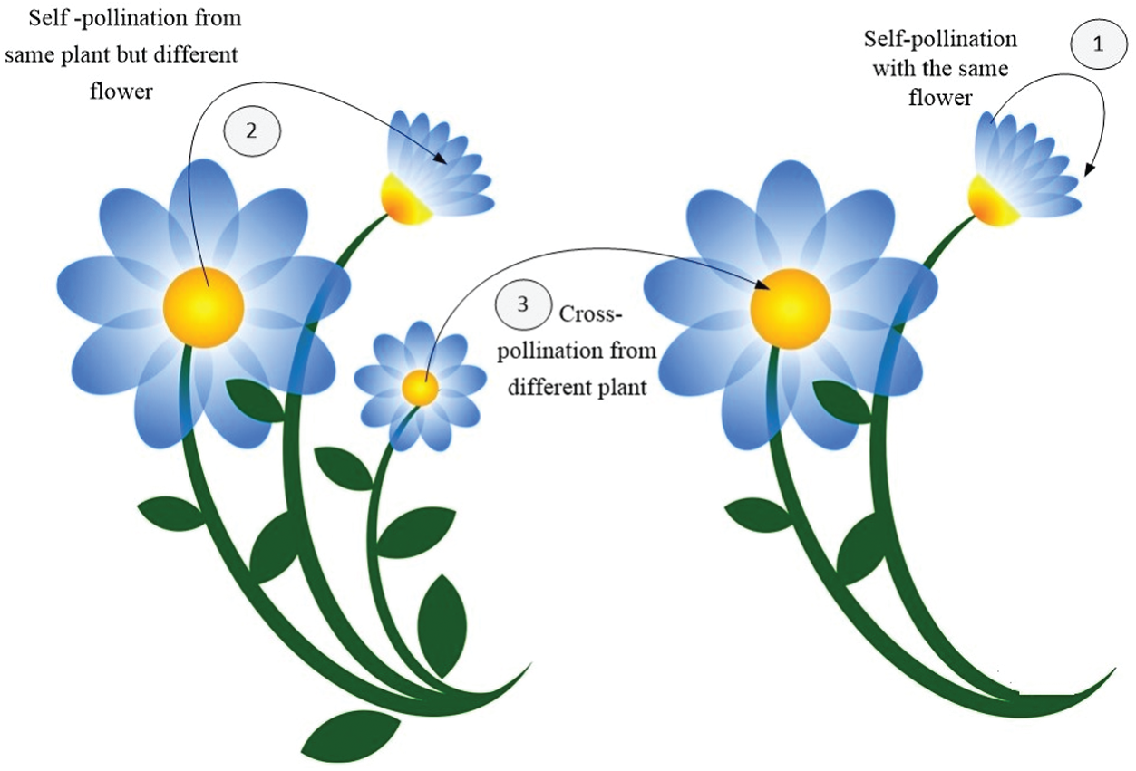
Figure 1: Process of flower pollination

The same is the operating procedure of FPA. It has local and global pollination. Whether the pollination is going to be global or local, it depends on probability switch P∈[0,1].

The characterization of global pollination is done by Eq. (1):

xit+1=xit+γL(λ)(gbest-xit)(1)

L(λ) is the Levy factor. It carries the transfer of pollens to different species of plant. It also determines the strength of pollination. γ is a scaling factor which controls the step size.

L(λ)=λΓ(λ)sin(πλ2)π1s1+λ(s≫s0>0)(2)

where Γ(λ) is the standard gamma function.

The characterization of local pollination is done by equation:

xit+1=xit+ε(xkt+xjt)(3)

‘ε’ represents the local search which is of uniform distribution ε∈[0,1]. xkt and xjt are different pollens of species of plants. The probability switch controls between global and local pollination. It’s optimal value is 0.8. The Flow Chart of FPA is shown in Fig. 2.

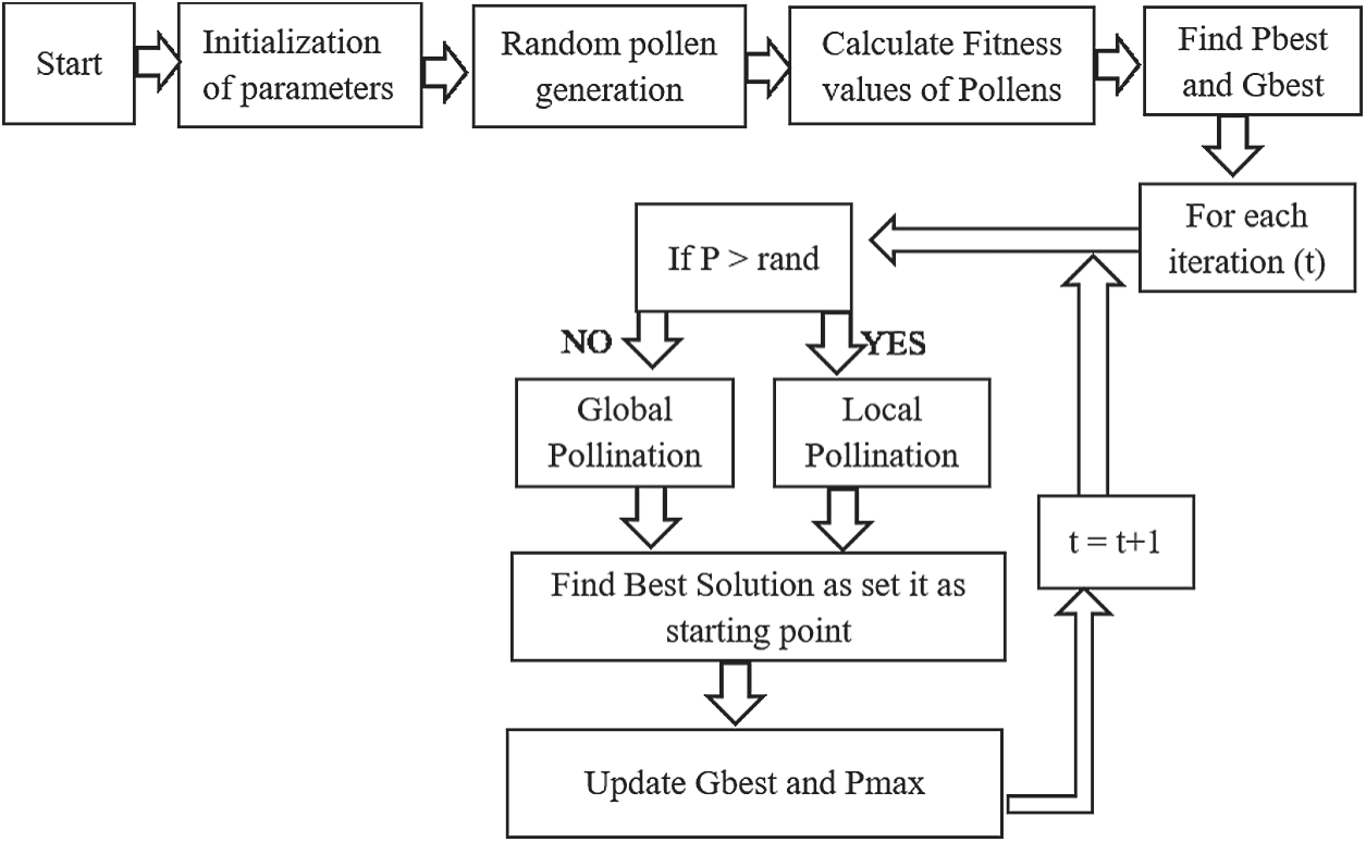
Figure 2: Flow chart of FPA

Initially random pollens (duty cycles) are generated and applied to Boost Converter which calculates power produced by each pollen. Among these pollens, it selects the best pollen which has maximum power among the group. Then that result is passed through a probability switch which determines if it’s going to be global pollination or local. After passing all the pollens through this process the pollen with Pbest is selected and that pollen is named Gbest. Now the system keeps running on the same duty cycle until irradiance changes. Once irradiance changes, the process is again repeated to search for new Gbest and Pbest.

The objective function for reaching maximum power is:

Pit+1>Pit(4)

2.2 Opposition-Based-Learning

The fundamentals of machine learning are learning, optimization, and searching. A learning algorithm learns from its past data/ instructions, optimizes estimated solutions, and searches for existing solutions.

Let’s suppose there is a problem and x is the solution. We estimate x^ based on experience or a random guess. x^ is not the exact solution but an estimate. If random guesses are not far away from the original solution then it makes convergence faster. If we have no prior knowledge then of course random guess can’t be correct. So we have to search the whole search space for the solution nearest to the original solution. Let’s say, in the worst case, the guess is the opposite point in the plane. It will take more time. But if we believe that an opposite point can be fruitful in the optimization of the solution then finding the opposite solution is the foremost task.

Lets say ‘x∈ℜ’ be a real number defined in [a,b] then x0 (the opposite of x) is defined as:

x0=a+b-x(5)

Lets say P(x1,x2,x3,…,xn) be a point in an n-dimensional coordinate system where x1,x2, x3,…,xn∈ℜ and xi∈[ai,bi]. The opposite point is defined by its coordinates x10,x20,x30,…,xn0 as:

xio=ai+bi-xi;i=1,2,3…n(6)

So the OBL can now be characterized as:

Let f(x) be a function and g(⋅) be its evaluation function. If x∈[a,b] is an initial random guess and x0 is its opposite value then in every iteration we can calculate f(x) and f(x0). The learning continues with x if g(f(x))>g(f(x0)), otherwise x0.

The exemplary optimization for OBL is shown in Fig. 3 below. Let’s say ‘y’ is the original solution we are looking for, and ‘x’ is the random guess. ‘x0’ is the opposite of ‘x’ in the plane [a1,b1]. The one among x and x0 which is nearer to y is kept and the other is discarded. Similarly, the half part of the plane in which the discarded solution lies also gets excluded out of the search domain, and the remaining half of the plane is searched for other solutions. The process goes on unless we reach the nearest to the original solution.

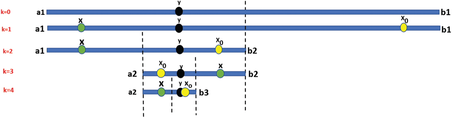
Figure 3: Opposition based learning optimization

2.3 Proposed Method

The random generation of pollens in FPA is vulnerable to fall into local maxima because of the uncertainty of the quality of initially generated pollens. So OBL method is applied in hybridization with FPA to improve the quality of random search through opposite solutions which makes sure that the system does not fall into local maxima. This leaves almost no room for global maxima to escape from the search. In this way, a more reliable method comes into being which is very effective and works in all shading conditions. The flow diagram of FPA-OBL is shown in Fig. 4.

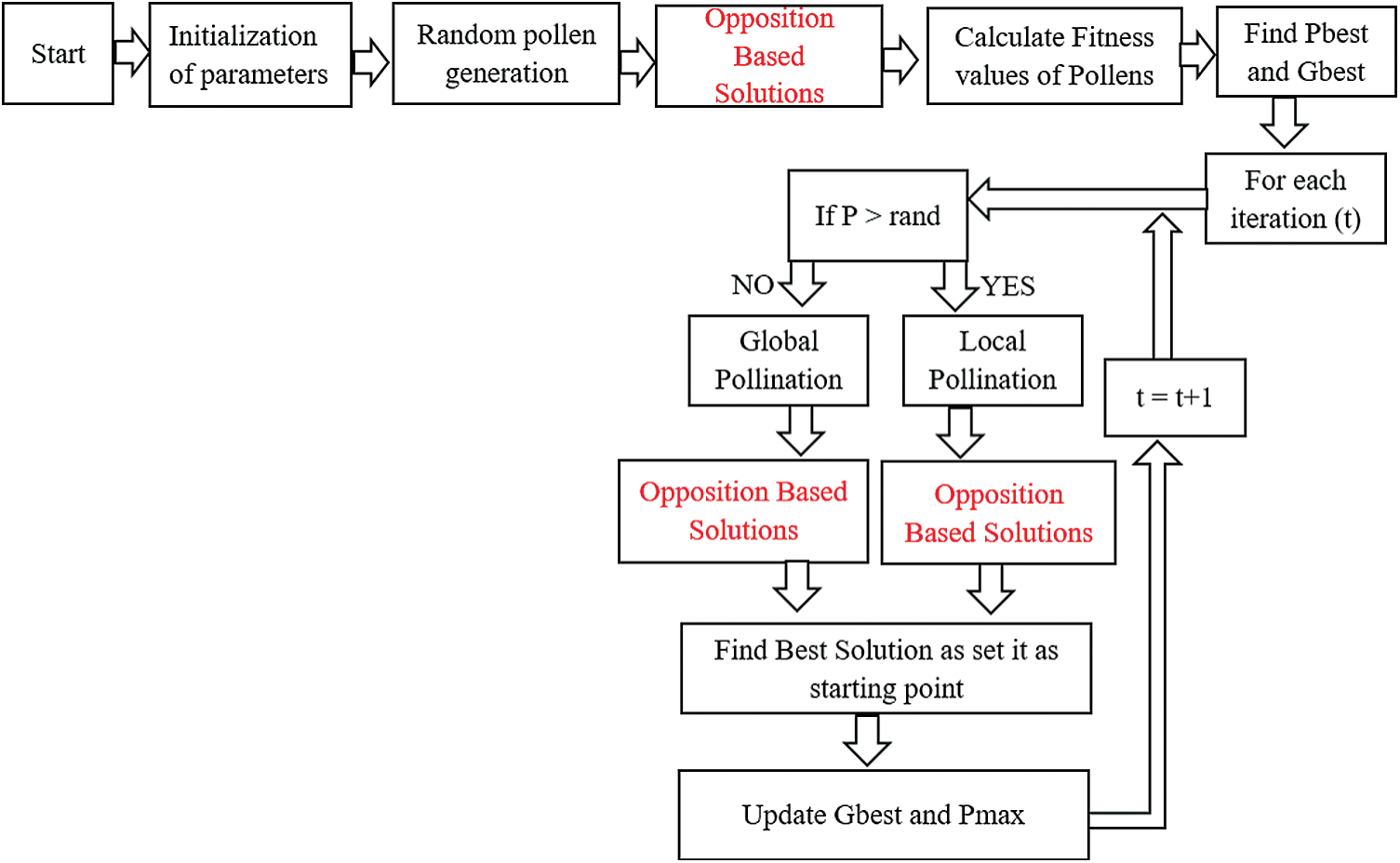
Figure 4: Flow diagram of FPA-OBL

3  Experimentation

Fig. 5 shows the proposed model for performing simulation analysis. The components used in the model and their values are briefly explained below.

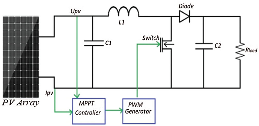
Figure 5: Model used for experimental analysis

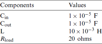
3.1 Values of Circuit Elements

The values of components used in the boost converter circuit are listed in Tab. 1.

Table 1: Values of components used in boost converter

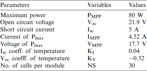
3.2 Model of PV Array Used and Its Characteristics

The model of the PV array used in this study is Sun Earth Solar Power TDB125xt25-36-P 80 W. The parameters of a single array with 1 parallel string and 1 series-connected module per string@1000 W/m2 irradiance are listed in Tab. 2.

Table 2: Module data/parameters of sun earth solar power TDB125xt25-36-P 80 W

The P-V characteristic curves of Sun Earth Solar Power TDB125xt25-36-P 80 W are shown in Fig. 6. Simulation studies in this work are carried out on arrays with each having 5 parallel strings and 1 series-connected module per string.

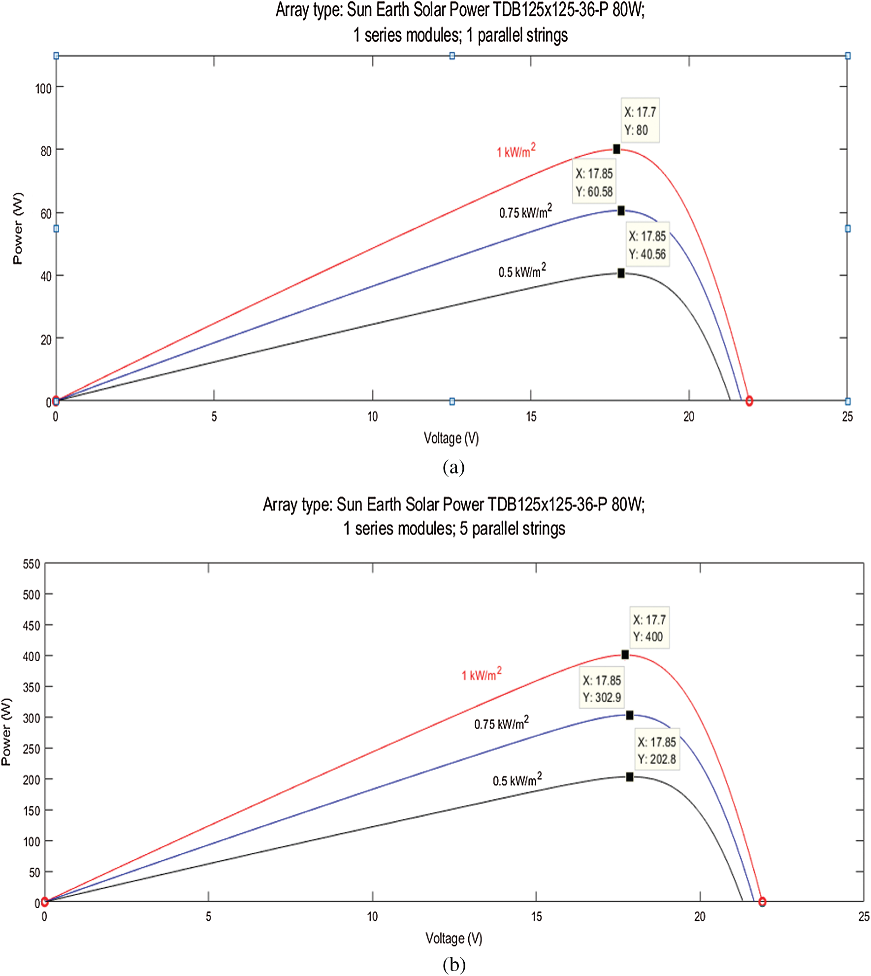
Figure 6: (a) P-V characteristic curves of sun earth solar power TDB125xt25-36-P 80 W with 1 parallel string and 1 series-connected module per string @ [1, 0.75, 0.5] kW/m2 irradiance. (b) P-V characteristic curves of sun earth solar power TDB125xt25-36-P 80 W with 5 parallel string and 1 series-connected module per string @ [1, 0.75, 0.5] kW/m2 irradiance

4  Simulations and Results

The validation of the proposed technique is done through the 3S1P & 3S2P configuration of arrays as shown in Fig. 7. Different case studies are performed to test the efficiency of the proposed method under different shading patterns. The input variables are irradiance (Irr) and temperature (T). Simulation studies are performed keeping temperature constant and assuming varying irradiance conditions.

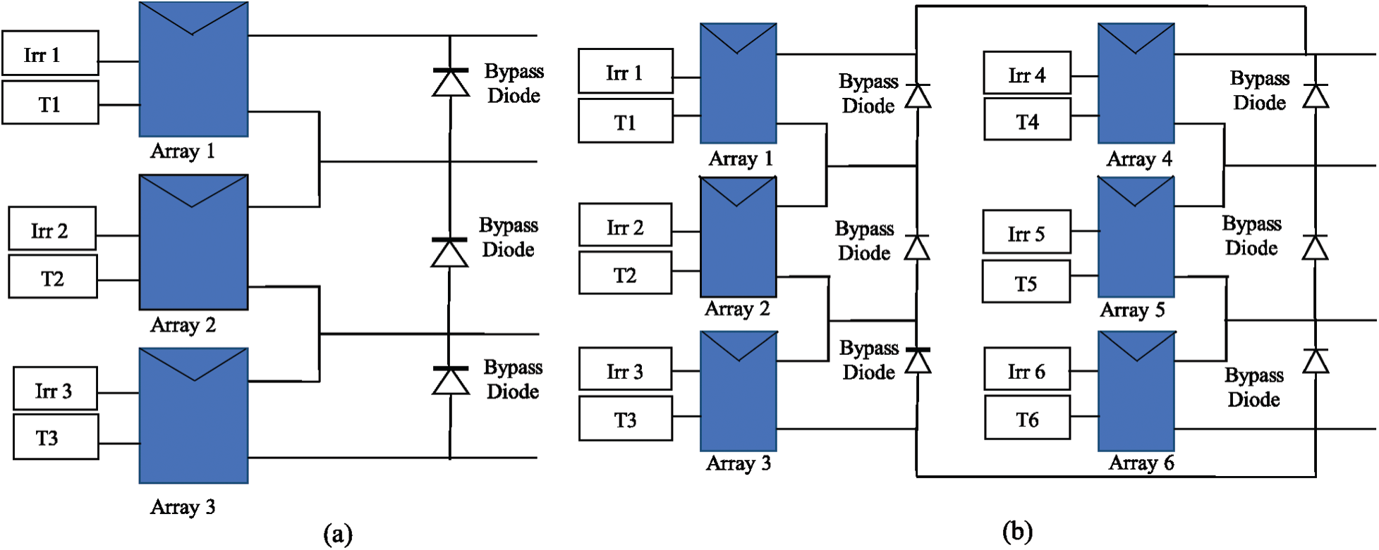
Figure 7: (a) 3S1P configuration of PV arrays (b) 3S2P configuration of arrays

4.1 3s1p Configuration

4.1.1 Case 1 (Zero Shading)

Case 1 presents a zero shading pattern in which all the arrays are facing the same irradiances (Irr-1, Irr-2, Irr-3=1000 W/m2) and no shading occurs on any array. Fig. 8a shows the rated P-V curve for the zero shading pattern. The rated power of this configuration is 1199.7 W. Figs. 8b & 8c show the output P-T and D-T curves of FPA, respectively. The extracted power of FPA is 1196.3 W at a duty cycle of 0.659. While Figs. 8d & 8e show the output P-T & D-T curves of FPA-OBL, respectively. The output power of FPA-OBL is 1199 W at 0.655 duty cycle.

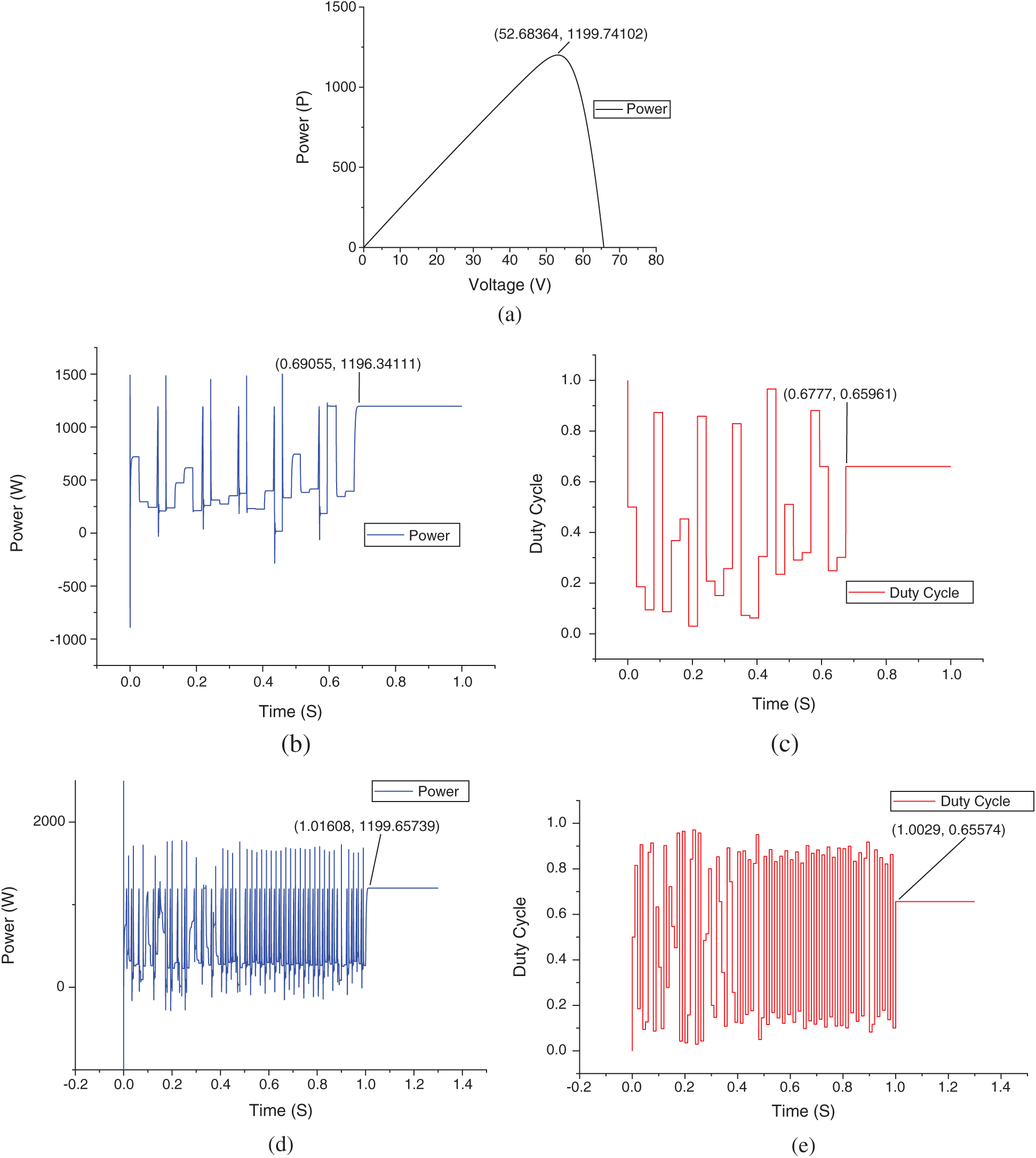
Figure 8: Case 1 (zero shading) (a) P-V curve (b) P-T curve of FPA (c) D-T curve of FPA (d) P-T curve of FPA-OBL (e) D-T curve of FPA-OBL

4.1.2 Case 2 (Weak Shading)

Case 2 presents a weak shading pattern in which the arrays are facing different irradiances (Irr-1=1000 W/m2, Irr-2 & Irr-3=500 W/m2) and a weak shading effect occurs. Fig. 9a shows the rated P-V curve for weak shading pattern. The rated power of this configuration is 640.79 W. Figs. 9b & 9c show the output P-T and D-T curves of FPA respectively. The extracted power of FPA is 637.3 W at a duty cycle of 0.5. While Figs. 9d & 9e show the output P-T & D-T curves of FPA-OBL respectively. The output power of FPA-OBL is 640.17 W at a 0.51 duty cycle.

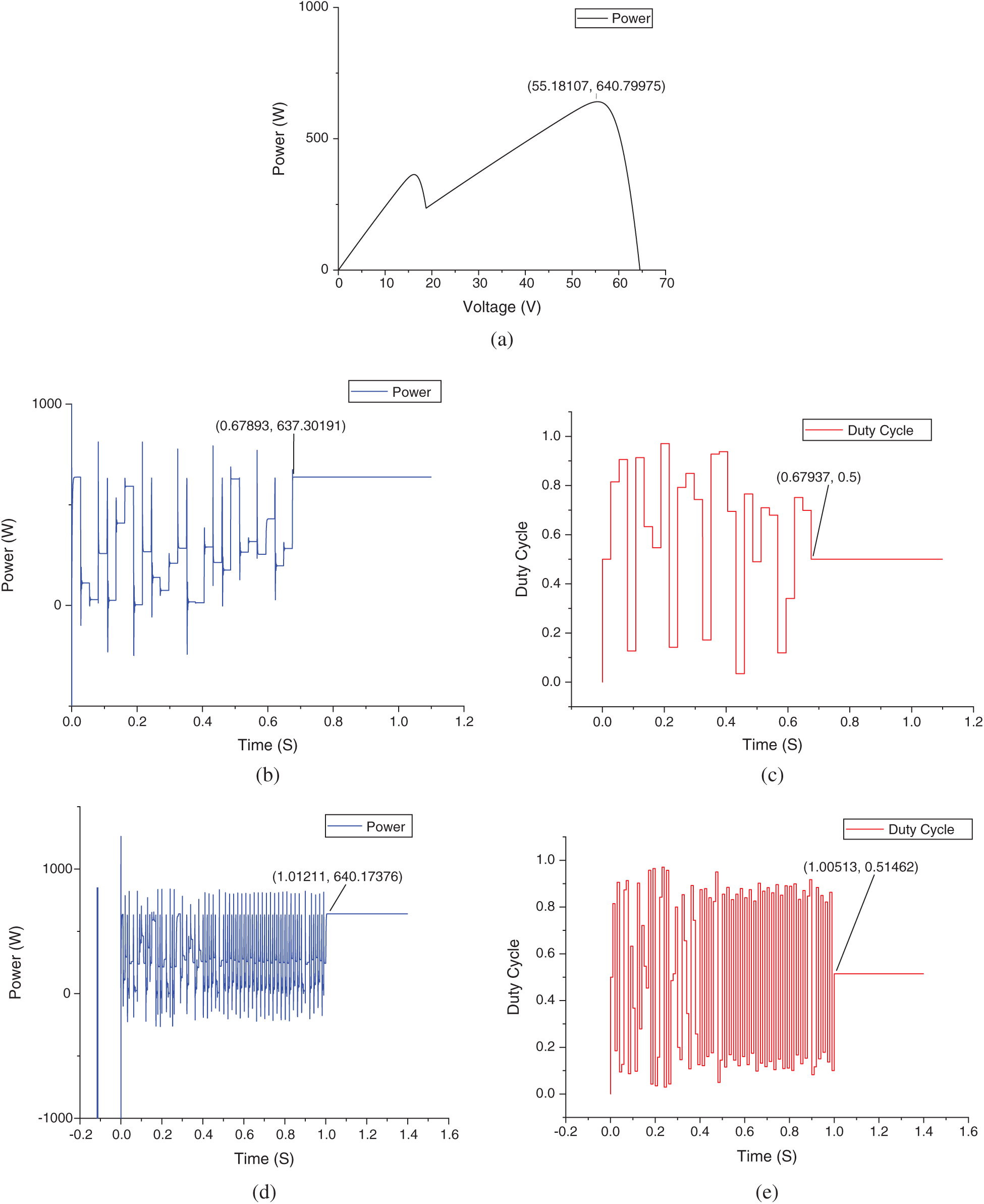
Figure 9: Case 2 (weak shading) (a) P-V curve (b) P-T curve of FPA (c) D-T curve of FPA (d) P-T curve of FPA-OBL (e) D-T curve of FPA-OBL

4.1.3 Case 3 (Strong Shading)

Case 3 presents a strong shading pattern in which all the arrays are facing different irradiances (Irr-1=1000 W/m2, Irr-2=750 W/m2, Irr-3=500 W/m2) and a strong shading effect occurs. Fig. 10a shows the rated P-V curve for a strong shading pattern. The rated power of this configuration is 672.53 W. Figs. 10b & 10c show the output P-T and D-T curves of FPA, respectively. The extracted power of FPA is 669.37 W at a duty cycle of 0.54. While Figs. 10d & 10e show the output P-T & D-T curves of FPA-OBL, respectively. The output power of FPA-OBL is 671.8 W at a 0.54 duty cycle.

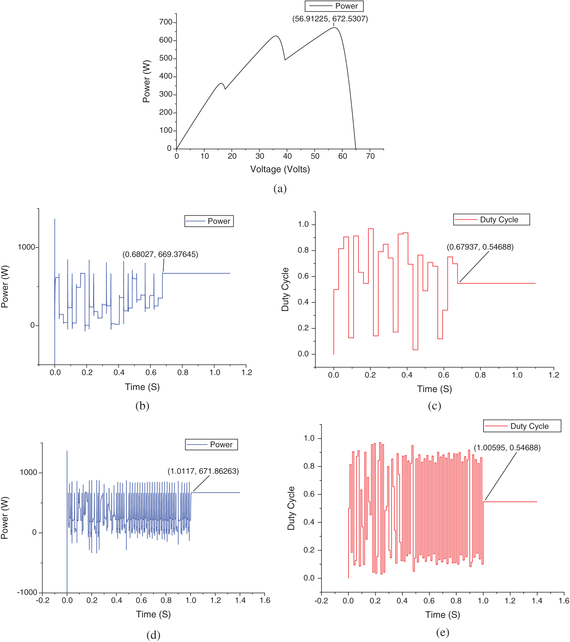
Figure 10: Case 3 (strong shading) (a) P-V curve (b) P-T curve of FPA (c) D-T curve of FPA (d) P-T curve of FPA-OBL (e) D-T curve of FPA-OBL

4.2 3s2p Configuration

The results of simulations of the 3s2p configuration are shown in graphical form in Fig. 11 below.

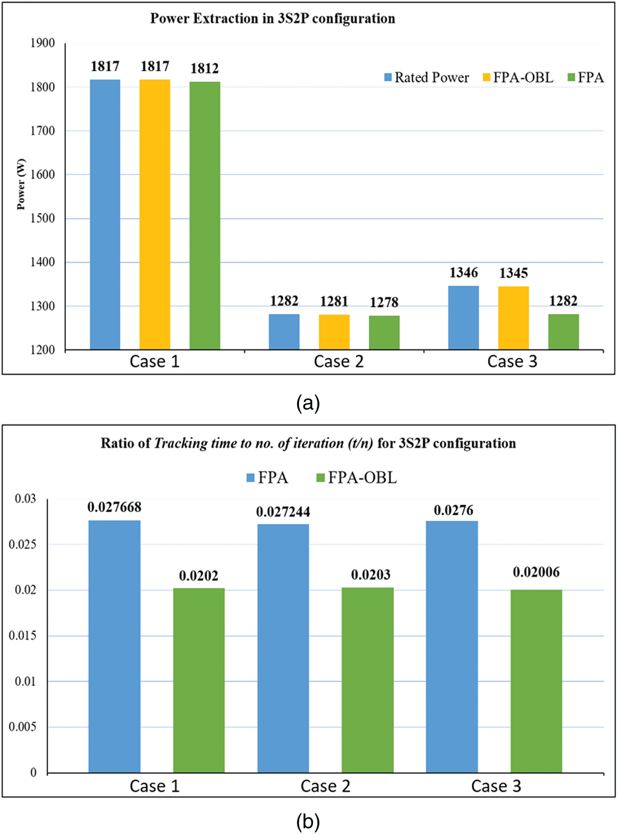
Figure 11: 3S2P configuration (a) power extraction of FPA and FPA-OBL (b) t/n ratio of FPA and FPA-OBL

5  Discussions and Comparison

5.1 Power Extraction

Power extraction depends upon the MPP. In partial shading conditions, abrupt changes in irradiance cause multiple peaks in the P-V curve. Every peak is a local peak but the highest among all is called the global peak. Classic MPPT method falls to local peaks and considers it as MPP which reduces the system output or extracted power. Figs. 8–11 show that the power extraction ability of FPA-OBL is better than FPA and its contemporaries in all cases. The results and comparison are shown in [18] and observations were done in this manuscript that proves the efficiency of the proposed method. The intelligent searching mechanism has a very effective GMPP tracking ability that has led to improved power extraction.

5.2 Convergence

As proved in [18] FPA has better convergence than P&O, IC, and HC. FPA-OBL has even better convergence than FPA as shown in the above simulations. This intelligent searching mechanism makes it easier to search the GMPP which improves the convergence of the proposed method. The classic methods have a typical search behavior and still, they are more likely to fall into local maxima and mislead the system. But FPA-OBL has this outstanding ability to find GMPP no matter what the shading conditions are. Having a fast converging and more accurate mechanism is an ideal situation for an MPPT algorithm so the proposed method has this quality.

5.3 Oscillations Around MPP

Usually during the MPP search process, when a system reaches its MPP it does not get settle there without any oscillations because the behavior of the mechanism makes the system do that. These oscillations give us a fluctuating power at the output which is not a good quality for a system. But in the case of FPA and FPA-OBL, there are no oscillations as their operating mechanism is better. There are no oscillations around MPP of both FPA and FPA-OBL. The other methods like P&O, IC, and HC have oscillations around MPP which give an unstable MPP. Figs. 8–10 justify this statement.

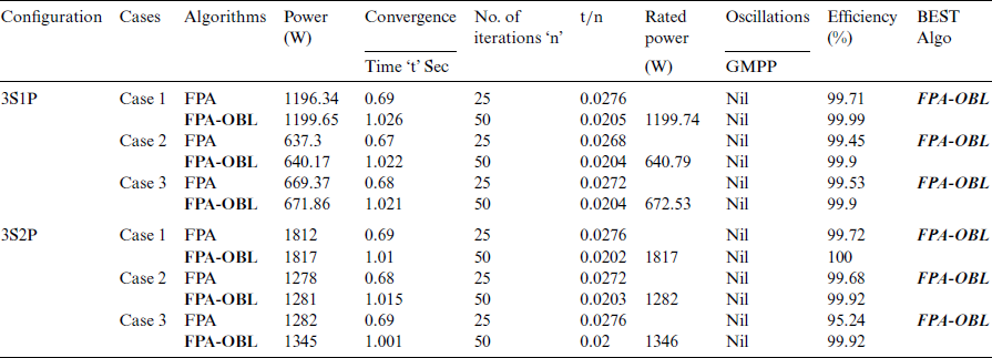
Tab. 3 presents the simulation studies in tabular form which sums up the whole discussion. It is evident from the table that FPA-OBL outperforms FPA in all configuration cases.

Table 3: Comparison of FPA and FPA-OBL

5.4 Comparison of FPA & FPA-OBL with Other MPPT Techniques

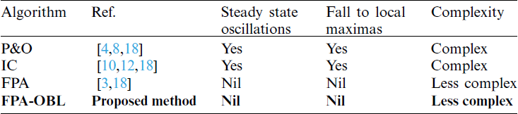
A comparison was made in [18] among FPA, P&O and IC algorithms which proved that FPA was better in partial shading as compared to other techniques. In [18] its proved that FPA has a better search mechanism, fewer parameters (which make it computationally better) and less complexity. All these qualities are incorporated in FPA-OBL with some more additions. Here in this research study, it has been seen that FPA-OBL has even better performance than FPA. Which makes it better than P&O and HC algorithms also. A comparison of some attributes of techniques is shown in Tab. 4.

Table 4: Comparison of Parameters of FPA, FPA-OBL, P&O, and IC

6  Conclusion

Harvesting of Solar energy has been under consideration for long and many conventional techniques had been proposed but they had a lot of problems related to them i.e., falling to a local peak when it’s a multipeak curve and oscillations around a steady state. Partial shading is one of the most known problems when it comes to addressing challenges faced to operate the PV module at MPP. In this study, an improved FPA algorithm is proposed to achieve maximum output from a PV array which is effective in all conditions of shading whether it is zero shading, weak shading, or strong partial shading. Simulation studies have proved that FPA-OBL is 0.25%–0.45% better in power extraction than FPA and its t/n ratio is also lower than FPA. It is proved that FPA-OBL is more efficient, less complex, more robust, and more flexible than FPA and other techniques.

Funding Statement: This work has been supported by the Xiamen University Malaysia Research Fund XMUMRF Grant No: XMUMRF/2019-C3/IECE/0007 (received by R. M. Mehmood). The authors are grateful to the Taif University Researchers Supporting Project Number (TURSP-2020/79), Taif University, Taif, Saudi Arabia for funding this work (received by M. Shorfuzzaman).

Conflicts of Interest: The authors declare that they have no conflicts of interest to report regarding the present study.

This work is licensed under a Creative Commons Attribution 4.0 International License, which permits unrestricted use, distribution, and reproduction in any medium, provided the original work is properly cited.