Computers, Materials & Continua DOI:10.32604/cmc.2021.014984
Article

Evaluating the Risk of Disclosure and Utility in a Synthetic Dataset

Kang-Cheng Chen1, Chia-Mu Yu2,*and Tooska Dargahi3

1Industrial Technology Research Institute, Hsinchu, 310, Taiwan
2National Chiao Tung University, Hsinchu, 320, Taiwan
3University of Salford, Manchester, M5 4WT, United Kingdom
*Corresponding Author: Chia-Mu Yu. Email: chiamuyu@gmail.com
Received: 31 October 2020; Accepted: 13 January 2021

Abstract: The advancement of information technology has improved the delivery of financial services by the introduction of Financial Technology (FinTech). To enhance their customer satisfaction, Fintech companies leverage artificial intelligence (AI) to collect fine-grained data about individuals, which enables them to provide more intelligent and customized services. However, although visions thereof promise to make customers’ lives easier, they also raise major security and privacy concerns for their users. Differential privacy (DP) is a common privacy-preserving data publishing technique that is proved to ensure a high level of privacy preservation. However, an important concern arises from the trade-off between the data utility the risk of data disclosure (RoD), which has not been well investigated. In this paper, to address this challenge, we propose data-dependent approaches for evaluating whether the sufficient privacy is guaranteed in differentially private data release. At the same time, by taking into account the utility of the differentially private synthetic dataset, we present a data-dependent algorithm that, through a curve fitting technique, measures the error of the statistical result imposed to the original dataset due to the injection of random noise. Moreover, we also propose a method that ensures a proper privacy budget, i.e., ϵ will be chosen so as to maintain the trade-off between the privacy and utility. Our comprehensive experimental analysis proves both the efficiency and estimation accuracy of the proposed algorithms.

Keywords: Differential privacy; risk of disclosure; privacy; utility

1  Introduction

Financial Technology (FinTech) concept has evolved as a result of integrating innovative technologies into financial services, e.g., AI and big data, Blockchain and mobile payment technologies, to provide better financial services [1]. Investments in FinTech industry is trending upward, such that by September 2020 the global investment in Fintech was $25.6 Billion, reported by KPMG [2]. However, security and privacy of the users’ data is among the main concerns of the FinTech users [3]. Data governance and user data privacy preservation are reported as the most important challenges in FinTech due to the accessibility of user data by suppliers and third parties [3]. Some financial institutions rely on honest but curious FinTech service providers which might be interested in accessing sensitive attributes of users’ data. Specially, in the case of small and medium businesses, which provide personalized financial services to their customers, with no background knowledge in security and data privacy, protection of users’ data becomes even more challenging.

The “open data” concept and data sharing for banking industry has been promoted by several countries, including the UK. A report by the Open Data Institute, discusses the benefits of sharing anonymized bank account data with the public and suggests that such data release could improve customers decision making [4]. User data are usually shared with the data consumers via data release; herein, we consider scenarios in which data are released, i.e., where tabular data with numeric values (which could be related to user’s bank transactions, stock investments, etc.) are to be published (or shared) by the data owner. However, data release often presents the problem of individual privacy breach, and there has always been a debate between data privacy and openness, reported by Deloitte [5]. A real-world example thereof is that, by using publicly available information, researchers from the University of Melbourne were able to re-identify seven prominent Australians in an open medical dataset [6]. Furthermore, researchers from Imperial College London found that it would be possible to correctly re-identify 99.98% of Americans in any dataset by using 15 demographic attributes [7]. Other relevant privacy incidents were also reported [8,9]. All of these incidents provide evidence of privacy leakage because of improper data release.

Recently, the United States and Europe launched new privacy regulations such as the California Consumer Privacy Act (CCPA) and General Data Protection Regulation (GDPR) to strictly control the manner in which personal data are used, stored, exchanged, and even deleted by data collectors (e.g., corporations). Attempts to assist law enforcement have given rise to a strong demand for the development of privacy-preserving data release (PPDR) algorithms, together with the quantitative assessment of privacy risk. Given an original dataset (the dataset to be released), PPDR aims to convert the original dataset into a sanitized dataset (or a private dataset) such that privacy leakage by using the sanitized dataset is controllable and then publish the sanitized dataset. In the past, the former demands could be satisfied by conventional approaches such as k-anonymity, l-diversity, and t-closeness. However, these approaches have shortcomings in terms of syntactic privacy definition and the difficulty in distinguishing between quasi-identifiers and sensitive attributes (the so-called QI fallacy), and therefore are no longer candidates for PPDR. In contrast, differential privacy (DP) [10] can be viewed as a de-facto privacy notion, and many differentially private data release (DPDR) algorithms [11] have been proposed and even used in practice. Note that DPDR can be considered as a special type of PPDR with DP as a necessary privatization technique.

Although it promises to maintain a balance between privacy and data utility, the privacy guarantee of DPDR is, in fact, only slightly more explainable. Therefore, in the case of DPDR, it is difficult to choose an appropriate configuration for the inherent privacy parameter, privacy budget ϵ. More specifically, DP uses an independent parameter ϵ that controls the magnitude of the injected noise, yet the selection of ϵ such that the data utility is maximized remains problematic. On the other hand, although the value of ϵ affects the magnitude of noise, it has no direct relevance to the risks of data disclosure, such as the probability of re-identifying a particular individual. In other words, the choice of ϵ such that the privacy is meaningfully protected still needs to be investigated. In practice, there is no clear recommendation by the regulatory institutions in Fintech industry on the preferred anonymization technique which could address the challenge of preserving privacy while providing openness. This might be due to the unclarity of privacy guarantee versus utility in the existing DPDR algorithms. Thus, a strong demand exists to develop novel measures for the risk of disclosure (RoD) and utility for DPDR.

1.1 Related Work

In this section we present a brief review of studies on the differentially private data release and the risk of disclosure.

1.1.1 Differentially Private Data Release (DPDR)

Privacy-preserving data release (PPDR) methods have been introduced to address the challenge of the trade-off between privacy and utility of a released dataset. Several anonymization and privacy-enhancing techniques have been proposed in this regard. The most popular technique is k-anonymity [12], which uses generalization and suppression to obfuscate each record between at least k −1 other similar records. Due to vulnerability of the k-anonymity against sensitive attribute disclosure where attackers have background knowledge, l-diversity [13] and t-closeness [14] are proposed to further diversify the record values. However, all of these techniques are proven to be theoretically and empirically insufficient for privacy protection.

Differential privacy (DP) [10] is another mainstream privacy preserving technique which aims to generate an obfuscated dataset where addition or removal of a single record does not affect the result of the performed analysis on that dataset. Since the introduction of DP, several DPDR algorithms have been proposed. Here, we place particular emphasis on the synthetic dataset approach in DPDR. Namely, the data owner generates and publishes a synthetic dataset that is statistically similar to the original dataset (i.e., the dataset to be released). It should be noted that, since 2020, the U.S. Census Bureau has started to release census data by using the synthetic dataset approach [15]. DPDR can be categorized into two types: Parametric and non-parametric. The former relies on the hypothesis that each record in the original dataset is sampled from a hidden data distribution. In this sense, DPDR identifies the data distribution, injects noise into the data distribution, and repeatedly samples the noisy data distribution. The dataset constructed in this manner is, in fact, not relevant to the original dataset, even though they share a similar data distribution, and can protect individual privacy. The latter converts the original dataset into a contingency table, where i.i.d. noise is added to each cell. The noisy contingency table is then converted to the corresponding dataset representation. This dataset can be released without privacy concerns because each record can claim plausible deniability.

Two examples in the category of parametric DPDR are PrivBayes [16] and JTree [17]. In particular, PrivBayes creates a differentially private but high-dimensional synthetic dataset D by generateing a low-dimensional Bayesian network N. PrivBayes is composed of three steps: 1) Network learning, where a k-degree Bayesian network N is constructed over the attributes in the original high-dimensional dataset O using an (ϵ/2)-DP algorithm; here k refers to a small value dependent on the affordable memory size and computational load. 2) Distribution learning: an (ϵ/2)-DP algorithm is used to generate a set of conditional distributions, such that each attribute-parent (AP) in N has a noisy conditional distribution. 3) Data synthesis: N and d noisy conditional distributions are used to obtain an approximation of the input distribution, and then from the approximate distribution, we sample tuples to generate a synthetic dataset D.

JTree [17] proposes to use Markov random field, together with a sampling technique, to model the joint distribution of the input data. Similar to PrivBayes, JTree consists of four steps: 1) Generate the dependency graph: The goal of this step is to calculate the pairwise correlation between attributes through the sparse vector technique (SVT), leading to a dependency graph. 2) Generate attribute clusters: Once the pairwise correlation between attributes is computed, we use junction tree algorithm to generate a set of cliques from the above dependency graph. These attribute cliques will be used to derive noisy marginals with the minimum error. 3) Generate noisy marginals: We generate a differentially private marginal table for each attribute cluster. After that, we also apply consistency constraints to each differentially private marginal table, as a post-processing, to enhance the data utility. 4) Produce a synthetic dataset: From these differentially private marginal tables, we can efficiently generate a synthetic dataset while satisfying differential privacy. Other methods in the category of parametric DPDR include DP-GAN [18–20], GANObfuscator [21], and PATE-GAN [22].

On the other hand, Priview [23] and DPSynthesizer [24] are two representative examples in the category of non-parametric DPDR. Priview and DPSynthesizer are similar in that they first generate different marginal contingency tables. The main difference between parametric and non-parametric DPDR lies in the fact that the former assumes a hidden data distribution, whereas the latter processes the corresponding contingency table directly. Specifically, noise is applied to each cell of the contingency tables to derive the noisy table. Noisy marginal contingency tables are combined to reconstruct the potentially high-dimensional dataset, followed by a sophisticated design of the post-processing step for further utility enhancement. Other methods in the category of non-parametric DPDR include DPCube [25], DPCopula [26], and DPWavelet [27].

1.1.2 Risk of Disclosure (RoD) Metrics

Not much attention has been paid to develop RoD, although DP has its own theoretical foundation for privacy. The research gap arises because the privacy of DP has been hidden in the corresponding definition, according to which the query results only differ negligibly from those of neighboring datasets. However, in the real world setting, the user prefers to know whether (s)he will be re-identified. Moreover, the user wants to know what kind of information is protected, what the corresponding privacy level is, and the potentially negative impact of the perturbation for the statistical analysis tasks. On the other hand, although many DPDR algorithms have emerged, because of the lack of a clear and understandable definition of RoD, we know that the choice of ϵ is critical but it hinders the practical deployment of DPDR systems. Thus, we eager to develop an RoD to quantitatively answer questions such as what kind of information is protected, what the corresponding privacy level is, and the potentially negative impact of the perturbation for the statistical analysis tasks properly.

To make the privacy notion easy to understand by layperson, Lee et al. [28] made the first step to have a friendly definition of the RoD. They adopt the cryptographic game approach define the RoD. Specifically, given a dataset O with m records, the trusted server randomly determines, by tossing a coin, whether a record r∈O will be deleted. Let D be the resulting dataset after the deletion of the chosen record. The attacker’s objective is to determine whether the record r exists. Here, the attacker is assumed to be equipped with an arbitrary knowledge of the datasets O and D. In this sense, Lee and Clifton formulated the attacker as a Bayesian attacker, which means that the attacker is aimed to maximize the probability of guessing correctly by using both the prior and posterior knowledge of O, D, and r.

Hsu et al. [29], on the other hand, propose to choose the parameter ϵ based on an economic perspective. The idea behind their work is based on the observation that a normal user has a financial incentive to contribute sensitive information (if the third party or even attacker provide the financial compensation). Their economics-inspired solution [29] can calculate an proper ϵ by striking a balance between the accuracy of the released data and ϵ. In addition, Naldi et al. [30] calculated the parameter ϵ according to estimation theory. More specifically, Naldi et al. put their emphasis only on the counting query (as the counting query leads to the minimal sensitivity) and define their RoD. Their solution is similar to the solution in this paper. Nonetheless, the restriction on the counting query implies the limited practicality. Tsou et al. [31] also presented an RoD and their RoD is defined by restricting the confidence level of the magnitude of Laplace noise. With an observation that the data owner who wants to evaluate the RoD is only in possession of an original dataset O and a candidate differentially private synthetic dataset D. With another observation that the magnitude of Laplace noise can be bounded with high probability, the value range of the Laplace noise can then be estimated with a certain confidence level. As a result, the estimated value range of the Laplace noise can be used to determine the level of distortion for the record values, and this also implies the privacy level.

1.2 Problem Statement

The assessment of the RoD and data utility of the DP synthetic dataset presents the following two difficulties.

•    RoD requires good explainability for layman users in terms of a privacy guarantee, while simultaneously allowing quantitative interpretation to enable the privacy effect of different DPDR algorithms to be compared. In particular, although the privacy budget ϵ in DP has a mathematical explanation, it is difficult for layman users to comprehend the meaning behind the definition. Moreover, the privacy budget is inconsistent with the requirements in the current privacy regulations such as GDPR and CCPA, because the relation between ϵ and legal terms such as “single-out” remains to be investigated.

•    Usually, it is necessary to generate a synthetic dataset and then estimate the corresponding privacy level by calculating the RoD. Nonetheless, this process requires an uncertain number of iterative steps until the pre-defined privacy level is reached, leading to inefficiency in synthetic dataset generation. Thus, the aim is to develop a solution that can efficiently estimate the privacy level of the DP synthetic dataset.

Though the methods in Section 1.1 can be used to determine ϵ (or to quantify the privacy level), all of them have inherent limitations as mentioned previously. In particular, two of these studies [28,29] can apply only in the case of interactive DP, where the data analyst keeps interacting with the server and receives query results from the server. Nevertheless, as interactive DP suffers from the privacy budget completion problem, the DPDR in this paper only considers non-interactive DP (see Section 2.1), which results in the publication of the differentially privacy dataset allowing an arbitrary number of queries. Thus, the studies [28,29] are not applicable to the assessment of RoD. Moreover, though the method in [30] is somewhat related to non-interactive DP, its application is limited to the counting queries. Sarathy et al. [32] also have a similar limitation since their work only applies to numerical data. Lastly, Tsou et al. [31] method works only when the synthetic dataset is synthesized with the injection of Laplacian noise. Unfortunately, this is not always the case, because Laplacian noise leads to synthetic dataset with awful utility and therefore the data owner might choose alternatives. The design of PriBayes, JTree, Priview, and DPSynthesizer (in Section 1.1.1) similarly indicate that a more sophisticated design is used for DPDR, further limiting the applicability of this work [31].

1.3 Contribution

Our work makes the following two contributions:

•    We define a notion for evaluating the risk of disclosure (RoD) particularly for the DP synthetic dataset. The state-of-the-art DPDR algorithms decouple the original dataset from the synthetic dataset which makes it difficult to evaluate the RoD. However, we strive to quantify the RoD without making unrealistic assumptions.

•    We propose a framework for efficiently determining the privacy budget ϵ in DP, using the curve fitting approach, taking into consideration the desired trade-off between the data utility and privacy.

2  Preliminaries

2.1 Differential Privacy (DP)

The scenario in our consideration is a trusted data owner with a statistical database. The database stores a sensitive dataset. The database constructs and publishes a differentially private synthetic dataset for the public. In this sense, DP has been a de facto standard for protecting not only the privacy in the interactive (statistical database) query framework but also the (non-interactive) data release framework (see below).

There are two different kinds of DP scenarios, interactive and non-interactive. In the former, a dedicated and trusted server is located between the data analyst, who issues queries to the server (the data owner), and server (data owner). The server is responsible for answering the queries issued by data analyst. However, to avoid information leakage from query results, before forwarding the query result, the server will perturb it. Obviously, the interactive setting is cumbersome because in reality the data owner needs to setup a dedicated server. On the contrary, in the latter, the server (data owner) simply releases a privatized dataset to the public after the sanitization of dataset. During the whole process, no further interaction with anyone is needed. The synthetic dataset approach is a representative for non-interactive DP. Throughout the paper, we consider the non-interactive setting of DP (i.e., DPDR) unless stated otherwise.

Let ϵ and M be a positive real number and a randomized algorithm with the dataset as the input, respectively. We claim that M is ϵ-DP if, for all neighboring datasets D1 and D2 that differ at most one single record (e.g., the data of one person), and all subsets S of the image of M,

Pr[M(D1)∈S]≤eϵ×Pr[M(D2)∈S],(1)

where the parameter ϵ can be adjusted according to the tradeoff between utility and privacy; a higher ϵ implies lower privacy. Therefore, ϵ is also called the privacy budget because, the number of query responses is positively proportional the privacy loss. From the above definition, we can also know that DP provides a cryptographic privacy guarantee (from indistinguishability point of view) that the presence or absence of a specific record will not affect the algorithm significantly. From attacker’s point of view, (s)he cannot tell whether a specific record exists given the access of the algorithm output.

DP can be achieved by injecting a zero-mean Laplace noise [33]. Specifically, the noise sampled from a zero-mean Laplace distribution is added to perturb the query answer. Then, the data analyst only receives the noisy query answer. With two parameters on the mean and variance, Laplace distribution is determined jointly by ϵ and global sensitivity,

Δq= maxD1,D2∥q(D1)-q(D2)∥,(2)

of the query function q; that is, for any query q and mechanism M,

M(D)=q(D)+Lap(Δqϵ)(3)

is ϵ-DP, where Lap(Δqϵ) is a random variable that follows a zero-mean Laplace distribution. Apparently, as stated above, ϵ determines the tradeoff between privacy and data utility. DP features the sequential composition theorem, which states that by querying the dataset k times, if each noisy response satisfies ϵ-DP, then all the k queries achieve kϵ-DP together. In addition, DP involves post-processing, which states that any kind of data-independent processing of a noisy answer (ϵ-DP) does not compromise its privacy guarantee.

2.2 Voronoi Diagram

In our proposed algorithm in Section 3.2.3, we take advantage of the Voronoi Diagram, a mathematical concept which refers to partitioning a plane into adjacent regions called Voronoi cells to cover a finite set of points [34]. The definition of a Voronoi diagram is as follows [34,35]: Let X be a set of n points (called sites or generators) in the plane. For two distinct points x,y∈X the Voronoi region/cell associated to x is the set of all points in theplane that are closer to x than to any other point in the plane (i.e. the nearest neighbor to the point). In other words, the region associated to x is all the points in the plane lying in all of the dominances of y, i.e., region(x)=⋂y∈X-{x}dominance(x,y), where dominance(x,y)={p∈R2∣l2(p,x)≤l2(p,y)}, where l2 is the Euclidean distance. Due to specific geometrical structure of Voronoi diagrams and their simplicity in visual perception, they have been used by several research studies, such as file searching, scheduling and clustering [34]. Recently, the Voronoi diagram has also been used for preserving location privacy in various research studies [36–38]. In [36] the authors propose a privacy preserving model for mobile crowd computing to hide users in a cloaked area based on the Voronoi diagram. This paper takes advantage of the Voronoi diagram to provide k-anonymity for users in each Voronoi cell. In another study, Bi et al [38] combine local differential privacy and Voronoi diagram in order to preserve privacy in edge computing.

Compared to the state-of-the-art, in this paper we adopt Voronoi diagram in a completely different manner for evaluating the RoD in a differentially private synthetic dataset.

3  Proposed Approach for Evaluating Risk of Disclosure

In the following, we consider the setting of an original dataset O and the corresponding differentially private synthetic dataset D, both sized m×n and with numeric attributes A1,A2,…,An. Each record in O represents personal information; a concrete example of O is a medical dataset, where each record corresponds to the diagnosis of a patient. We do not assume a particular DPDR algorithm unless stated otherwise. The DPDR algorithms in Section 1.1.1 are all available for consideration. Our goal is to develop friendly notions of both RoD and utility, ensuring that these notions can easily quantify the RoD and utility of D, given the access to O and the satisfaction of ϵ-DP.

First, we discuss a simple metric for RoD in Section 3.1. In Section 3.2, we present four privacy notions. After that, we claim that the combined notion would be the best by justifying its self-explainability. Thereafter, we present our solution of how to quickly evaluate the utility of the synthetic dataset, given a specific privacy level, in Section 3.3. At last, we present in Section 3.4 a unified framework of calculating the maximal privacy budget ϵ by jointly considering utility and RoD.

3.1 Straightforward Metric for RoD

Irrespective of the approach that was followed to generate the synthetic dataset, each record in D could be “fake”; i.e., the existence or non-existence of a record in the synthetic dataset does not indicate the existence status of this record in the original dataset. In theory, even an attacker with abundant background knowledge cannot infer the individual information in O. Specifically, the privacy foundation lies in the fact that D is no longer a transformed version of O, and one cannot link O and D. Nonetheless, in reality, layman users are still concerned about the probability of the attacker re-identifying an individual from the synthetic dataset. We term this phenomenon the scapegoat effect. In particular, the scapegoat effect states that despite the fact that the information about an individual x in O will almost certainly not appear in D, because a record x^ in D could be sufficiently similar to x and the attacker only has partial knowledge of x, the attacker will (falsely) identify x^ as x. We claim the importance of the scapegoat effect because this is similar to the skewness attack in l-diversity [14]. In other words, an innocent individual might be accused of a crime if they are misclassified as either being or not being in the dataset.

Considering that most people may be concerned about the probability of an individual being re-identified by an attacker, given a synthetic dataset, a straightforward method for assessing the privacy level of the synthetic dataset would be to calculate the hitting rate, which is defined as the ratio of the number of overlapping records to the total number m of records in both datasets. Despite its conceptual simplicity, the use of the hitting rate incurs two problems.

•    First, because of the curse of dimensionality, the density of the data points in a high-dimensional space is usually low. This could easily result in a very low hitting rate and an overestimated level of privacy guarantee.

•    Second, such an assessment metric leads to a trivial algorithm for a zero hitting rate. For example, a synthetic dataset could be constructed by applying a tiny (and non-DP) amount of noise to each record in the original dataset. Owing to the noise, the records in the original and synthetic datasets do not overlap, leading to a zero hitting rate and an overestimated level of privacy.

3.2 Our Proposed Methods for RoD

In this section, we develop friendly privacy notions (or say friendly RoD estimation) from a distance point of view. More specifically, as we know from the literature, in the DPDR scenario, the original dataset O is already decoupled from the synthetic dataset D. A consequence is that there is no sense to connect between O and D. This also implies the difficulty in defining the appropriate RoD. However, the previous work [28–31] sought different ways to create the linkage between O and D, as the linkage between them is the most straightforward way for human understanding. Unfortunately, the privacy notion based on the linkage inevitably incurs security flaw, especially in the sense that such a linkage does not exist.

In the following, taking the scapegoat effect into consideration, a distance-based framework, (y,p)-coverage, is first proposed in Section 3.2.1 to minimize the scapegoat effect and to reconcile the privacy level and decoupling of O and D. The idea behind (y,p)-coverage is inspired by the observation that, even without the knowledge of the linkage between O and D, the only strategy left for the attacker is still to seek the closest record in O as the candidate original record in D. However, (y,p)-coverage is not suitable for measuring RoD because it has two parameters and does not have total order (described in more detail at the end of Section 3.2.1). Subsequently, we propose RoD metrics to measure the risk of re-identification.

3.2.1 (y,p)-Coverage

Here, we propose the notion of (y,p)-coverage as a framework for evaluating RoD. The idea behind (y,p)-coverage is that, the attacker would exhaustively search for a candidate matched record in O, given access to D. In particular, given Di as the ith record of D (ith row of D), due to the lack of pre-knowledge, the attacker’s research range would be in the neighborhood of a specific record Di. In this sense, the corresponding privacy metric can be formulated as a minimum weight bipartite matching problem in graph theory. Also from graph theory, we know that one can use the Hungarian Algorithm to handle minimum weight bipartite matching problem and so one can conduct the same algorithm to evaluate the RoD with the observation that O and D would be of the same size. In particular, Algorithm 1 is the pseudocode of the above idea, whose aim is to test if the distance-based (y,p)-coverage is fulfilled. Given O and D, we construct a complete weighted bipartite graph G=(V,E,W), where

V=O∪DandE={(Oi,Dj)}Oi∈O,Dj∈D.(4)

In the graph G, each edge has an edge weight that indicates the dissimilarity between the respective records; hence, the edge weights are defined as

W={eij}witheij=∥Oi-Dj∥.(5)

The graph G has 2m vertices, each of which corresponds to a record from O. Thus, each vertex can also be seen as an n-dimensional row vector. Under such a construction, G is completely bipartite as all the vertices from O are connected to all those from D. No direct edge for any pair of vertices both of which are for O (and D) exists. We also note that, the notation ∥⋅∥ denotes the norm. Here, while many norms can be used, an implicit assumption in this paper is that we always choose to use the Euclidean distance for ∥Oi-Dj∥=∥(χ1,…,χn)∥ for certain χ1,…,χn. However, the other norm can also be used as an alternative.

Given a matching M, let its incidence vector be x, where xij = 1 if (i,j)∈M and 0 otherwise, and the perfect matching of the minimum weight is a subset of edge weights such that

min∑i,jcijxij,(6)

where cij = wij. Once the Hungarian algorithm is performed, we can derive the perfect matching and the corresponding edge weight ω, where ω is an m-dimensional vector and the ith entry of ω denotes an edge weight of the minimum weighted bipartite matching for Di. We then calculate the number of weights less than or equal to y as a count ζ,

ξ=∑i=1mIωi≤y,(7)

where Iωi≤y denotes an indicator function with Iωi≤y=1 in the case of ωi≤y, and Iωi≤y=0 otherwise, given a user-defined weight y. Subsequently, we calculate p′=ζ/m. With the probability p from the user, D is supposed to fulfill (y,p)-coverage if p′≤p.

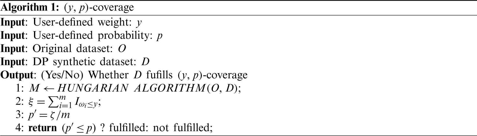
Despite its conceptual simplicity and theoretical foundation, (y,p)-coverage cannot be used for assessing RoD because (y,p)-coverage has two parameters y and p and does not have total order. Note that the purpose of developing the RoD metric is to enable layman users to conveniently choose the privacy budget ϵ in DP. However, when the notion of (y,p)-coverage is used, it may be difficult to determine which of, for example, (3,0.5)-coverage and (4,0.4)-coverage, improves the privacy. Hence, the following sections define additional privacy notions with total order to enable an RoD comparison.

3.2.2 y-Privacy

An underlying assumption for the (y,p)-coverage that the attacker conducts a search to look for a bijective matching between O and D by using the Hungarian algorithm. However, this assumption may fail in reality. To fit the reality setting, one can relax such an assumption, ensuring that the attacker instead performs an exhaustive search to find a matching between O and D. In this process, two records in D may happen to be matched against the same record in O. In (y,p)-coverage, we only keep one matching and get rid of another matching, which does not make sense. Therefore, in this section, we propose to use y-privacy to overcome the above limitation. While (y,p)-coverage can be seen as an average-case analysis, y-privacy is featured by its focuses on the worst-case analysis.

Algorithm 2 is proposed to achieve y-privacy; more specifically, it is used for verifying whether a given dataset satisfies y-privacy. In what follows, we consider the case of n = 1 with integral values in O to ease the representation. We will relax this assumption later. However, our implementation is a bit different from the above description. Instead, we in Algorithm 2 turn our focus to finding the mapping, instead of the matching, between O and D with the minimum incurred noise. First, we find the minimum value yi′ for each record Di in D such that [Di±yi′] contains one original record in O. This ensures that an original record is within the attacker’s search range. Then, for each yi′ in y′, we calculate

y′=argmin1≤j≤m∥Di-Oj∥.(8)

The above equation indicates that, because y can be seen as all of the possibilities, when the attacker sees a record, it needs to be verified whether this was a brute-force guess. Consequently, a lower y implies a downgrade privacy. Thus, Eq. (8) can also be seen as the probability that the attacker successfully makes a correct guess on an original record in O within the range [Di-y,Di+y], given that a record Di∈D is always at most 1/(2y + 1). One can also choose y′ in such a way that the median of y′ is selected as y to strike a balance between the privacy and utility. In comparison, the choice of y′ goes back to the average-case analysis, and choosing the minimum y′ as y has a similar flavor of (y,p)-coverage.

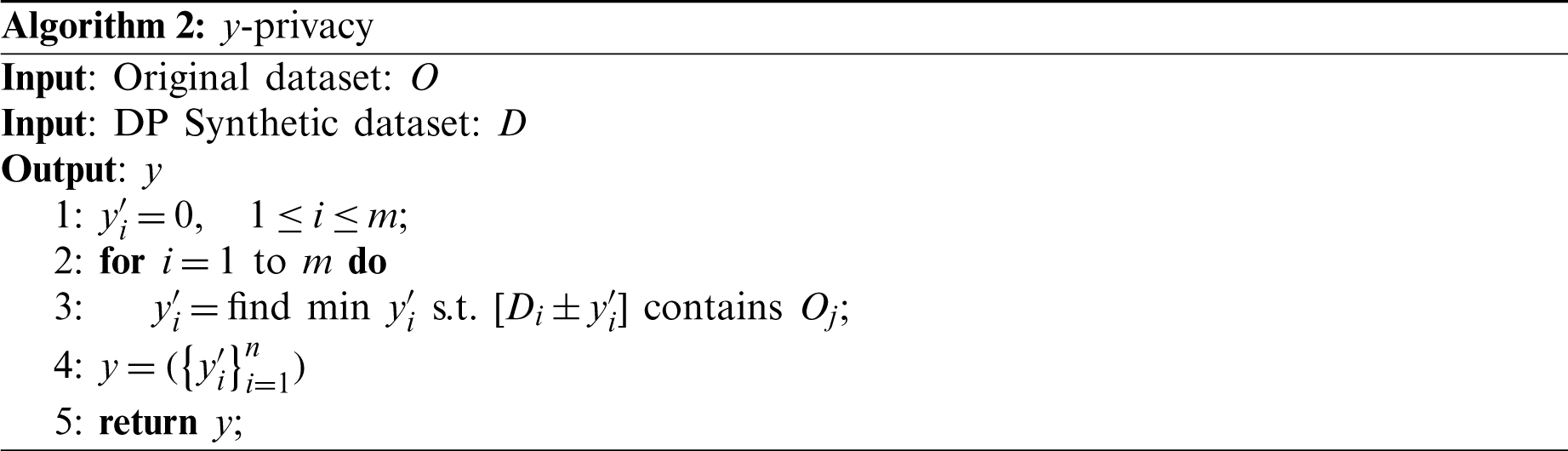
One can see that Algorithm 2 can also apply to the case of n≥2, once we properly define the operation [Di±yi′], because Di is n-dimensional. The definition can be derived by considering ∥Di-x∥≤y for all n-dimensional vectors x. The same patch can be used in the operation [Di±yi′] even if the record values are floating numbers.

Under the framework of (y,p)-coverage, y-privacy considers a general attack strategy and provides a worst-case guarantee. Compared to (y,p)-coverage, y-privacy has total order, and it is easy to see that y-privacy is better than y′-privacy when y≥y′ in terms of the privacy guarantee. Intuitively, the above argument that y-privacy is better than y′-privacy when y≥y′ also indicates that each record in the synthetic dataset satisfying y-privacy will be at least y-far away from the closest record in the original dataset, in contrast to the synthetic dataset, which satisfies y′-privacy. However, y-privacy is still not practical when a dense dataset (consisting of a huge number of records) is considered. Specifically, the common weakness of y-privacy and (y,p)-coverage is that when the records in a dataset are seriously dense, the parameter y in y-privacy and (y,p)-coverage should be very small. This can be understood by the fact that the records are close to each other both before and after the noise injection. It turns out that the parameter y becomes less meaningful as a privacy level.

3.2.3 Voronoi Privacy

The notion of y-privacy can also be generalized to consider its extreme condition. In other words, because y-privacy considers a y-radius ball centered at each data point and considers the number of data points in O covered by this y-radius ball, we can follow this perspective and consider the y-radius balls centered at all data points in O. The rationale behind the above consideration is to determine the arrangement of the dataset with the optimal y-privacy. Expanding the radius of all y-radius balls ultimately leads to a Voronoi diagram [39]. As explained in Section 2.2, this diagram is a partition of a multi-dimensional space into regions close to each of a given set of data points. Note that a Voronoi diagram can be efficiently constructed for two-dimensional data points, but for high-dimensional data points this would only be possible by using approximation algorithms [40,41]. The Voronoi diagram is characterized by the fact that, for each data point, a corresponding region consisting of all points of the multi-dimensional space exists closer to that data point than to any other. In other words, all positions within a Voronoi cell are more inclined to be classified as a particular data point.

From the perspective of RoD, we then have an interpretation that, in terms of y-privacy, each record in D cannot be located at these positions within the Voronoi cell; otherwise, an attacker who finds such a record in D is more inclined to link to a particular record in O. The above argument lies in the theoretical foundation of Voronoi privacy. Algorithm 3 shows the calculation of Voronoi privacy, given access to O and D. In particular, the rationale behind Voronoi privacy is to derive the optimal privatized dataset D^ (in terms of privacy) first, and then calculate the distance between D and D^ as an RoD metric. A larger distance implies a higher level of dissimilarity between D and D^ and therefore a lower risk of data closure.

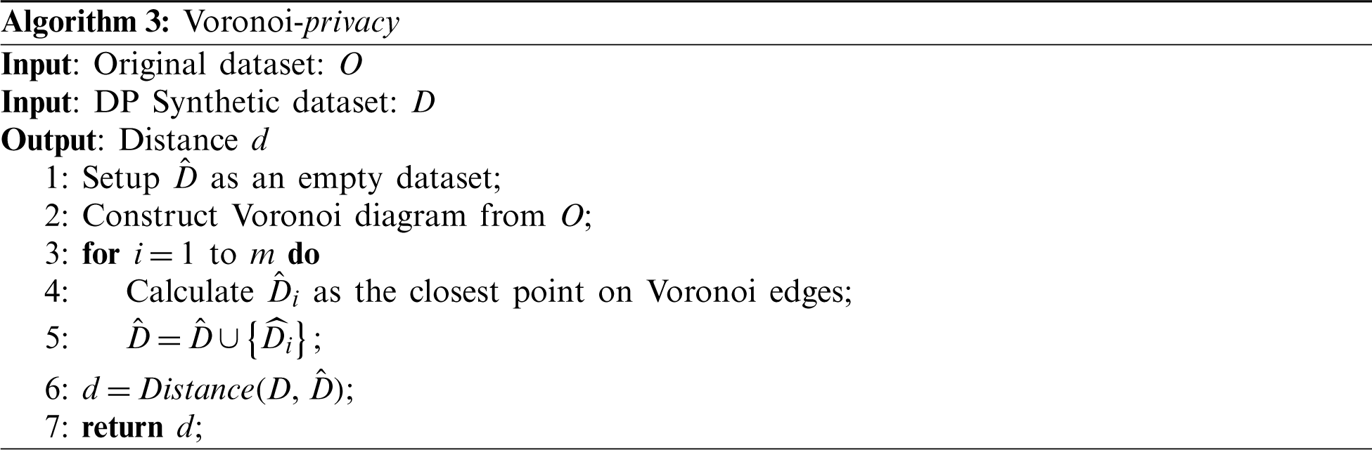
In this sense, first, Algorithm 3 constructs an empty dataset D^. The subsequent procedures gradually add records to D^, making it optimal in terms of privacy. Then, Algorithm 3 constructs a Voronoi diagram from O because the data owner would like to know the corresponding optimal privatized dataset. As mentioned previously, approximation algorithms [40,41] might be candidates for this task. Once the data owner has a Voronoi diagram from O, the collection of data points on the Voronoi diagram constitutes the optimal privatized dataset. Thus, an infinite number of optimal privatized datasets are available. Here, we aim to find the optimal privatized dataset with the optimal data utility. Considering that more perturbation on the record in O implies lower data utility, for each data point in O, the closest point on Voronoi edges would have been identified. The data owner collects all these data points as D^. Thereafter, the data owner calculates the distance between D and D^ as an RoD metric. We particularly mention that different choices of the Distance function are possible in the implementation, depending on the domain of the dataset. In general, the l2 distance (Euclidean distance) can be used, whereas the earth mover distance (EMD) could also be used if the data owner was interested in quantitatively measuring the data utility in terms of machine-learning applications.

3.2.4 p-Privacy

Based on the observation that dependency among attributes of the dataset can be a characteristic of the privacy, Algorithm 4 defines a novel privacy metric, called p-privacy. This is due to the fact that, in reality, the attacker will not perform a pure random guess; instead, the attacker would make educated guesses according to the distribution of O. The difficulty for the attacker is that (s)he does possess O. However, because D and O have the similar distribution according to the DPDR, the attacker can still make educated guesses by considering only the distribution of D. Inspired by this observation, we know that further reducing the futile combinations in the general case of n≥2 would be necessary. Thus, by computing the correlation among attributes (similar to JTree), our first step is to construct the dependency graph G. This step would be different from the exhaustive search in y-privacy and (y,p)-coverage. After deriving a dependency graph, we consider each linked part as a clique and obtain a clique set C. We calculate DCi, where DCi are records with values only for the attributes in Ci for each clique Ci in C. Let U be the set of DCi. Then, we produce a candidate table F with ∏i=1|U||DCi| combinations by merging each DCi in U to. The candidate table F can be seen as the records that more likely to be the records in O. Subsequently, after a comparison between F and O, one can find a count ξ, where the records of F belong to O, and then obtain the attack probability p,

p=ξ|F|⋅ξ|O|.(9)

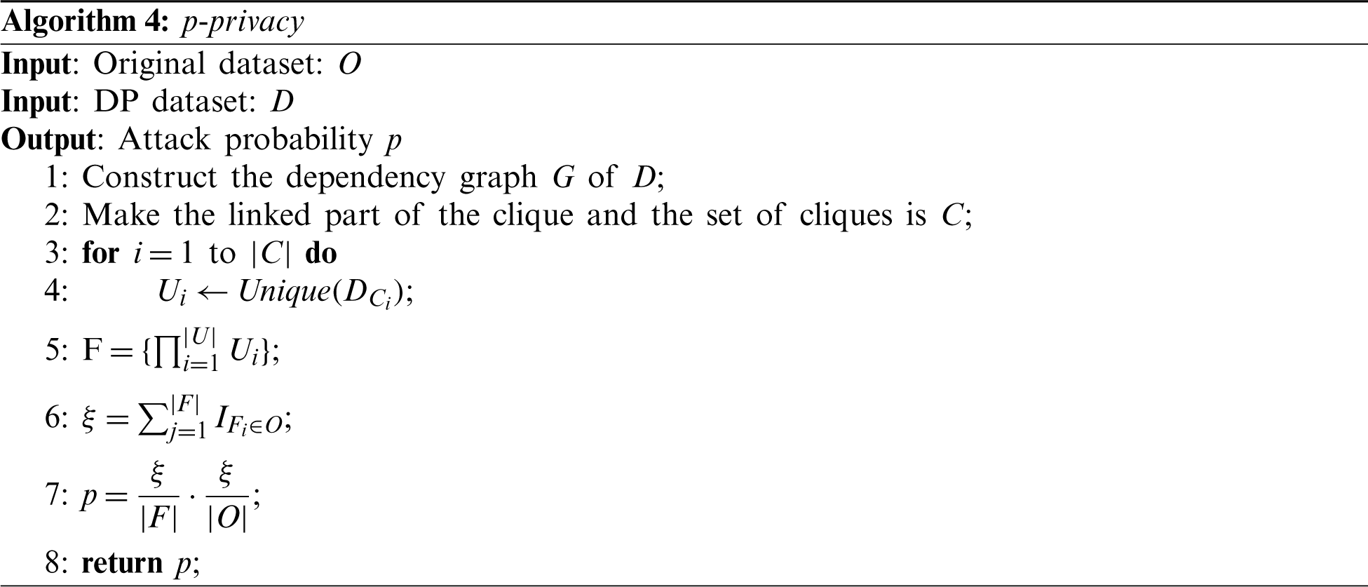
In the table below, we assume an exemplar original dataset O and synthetic dataset D. Based on this assumption, we show how p-privacy works to serve as a friendly privacy notion.

We have C={A1,A2,(A3,A4,A5)} after the lines 1 and 2 of Algorithm 4. Next, in the line 3 of Algorithm 4, we obtain U={(3,4,8),(1,5,7),[(1,2,3),(2,3,4)]}. In the line 4, we derive the following table F.

In Table F, both (3, 5, 1, 2, 3) and (8, 1, 2, 3, 4) exist in O. Therefore, in step 5, ξ will be 2. Finally, in the line 6 of Algorithm 4, p=218⋅23=227.

3.2.5 Data-Driven Approach for Determining ϵ

Although how to determine a proper privacy level (notion) is presented in Section 3.2.1~3.2.4, we still eager to develop a method for choosing an proper ϵ in DP for a given privacy level. In other words, in the previous sections, we only have a friendly explanation on the privacy but still need a concrete method to determine ϵ. In the following, based on the curve fitting technique, we propose algorithms to obtain satisfactory values for ϵ.

Baseline Approach for Determining ϵ. Inspired by JTree [42], Algorithm 5 adopts a similar strategy from JTree to determine the ϵ that satisfies the user’s risk and utility requirements. Apparently, if the O is uniformly distributed, only a small amount of noise will be needed to reach the desirable privacy level, because each record has the low sensitivity. However, if the data distribution of the original dataset is not uniform, additional noise is needed to protect the sensitive records, as stated in Section 2.1.

More specifically, the data owner can determine the sensitive records and the variance of Laplacian noise, given the marginal tables in JTree. Thus, we construct the corresponding dependency graph and calculate the marginal tables. Then, once we have a user-defined probability p that represents the preferable utility and privacy levels, the value of ϵ can be derived from the equation

noise=Lap(Δ(f)ϵ).(10)

The above procedures are similar to those in JTree, except that some operations are ignored. Moreover, as count queries are the fundamental operation that can have minimal impact on the function output, the global sensitivity Δ(f) is 1. So, the 95% confidence interval (μ+2σ) of Lap(1ϵ) is used in our consideration as the maximum value that represents p. This choice enables us to determine a satisfactory ϵ via Algorithm 5.

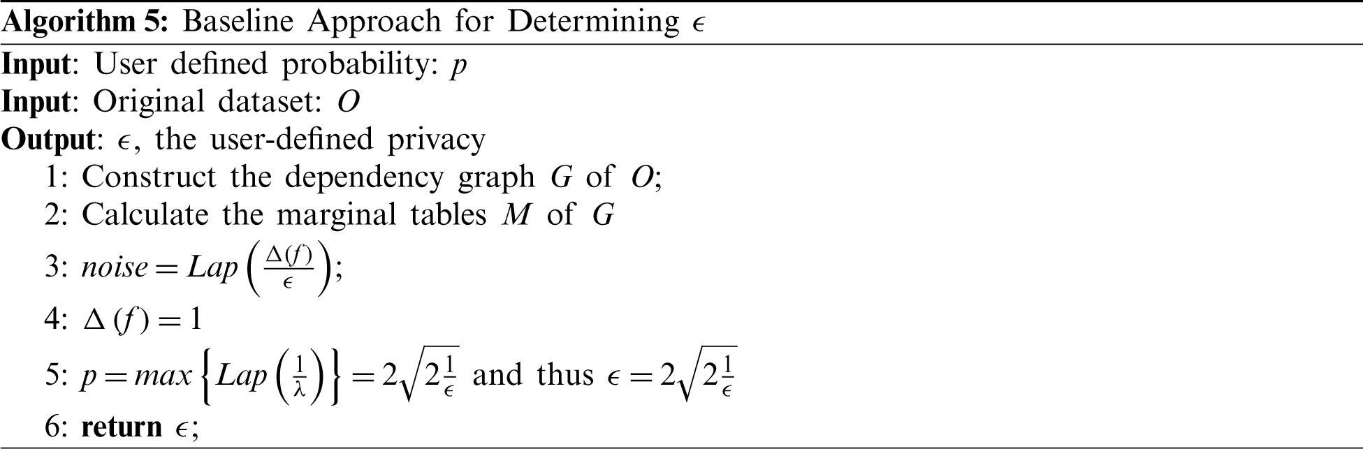
Unfortunately, Algorithm 5 poses certain problems, such as the possibility that, because different kinds of DP noise injection mechanisms could be used, one cannot expect that the ϵ retrieved from Algorithm 5 can be suitable for all of DP noise injection mechanisms. On the other hand, as the utility is closely related to ϵ, the choice of ϵ is also critical in improving the data utility. This makes it necessary to develop a more accurate method for estimating ϵ.

Data-Driven Approach for Determining ϵ. The simplest idea to determine ϵ is an iterative algorithm; i.e., we generate a synthetic dataset with a chosen ϵ and see whether the utility goes to be what we want. This is a theoretically feasible solution but is very inefficient, especially in the case of an uncertain number of iterations. Therefore, curve fitting, a data-driven approach, is proposed to learn the correlation between privacy level and ϵ. The curve bridges between privacy and utility. So, once we derive the curve, ϵ can be calculated instantly, given the desired level of utility. The remaining question is how we can derive the curve. The corresponding privacy levels can indeed be obtained after generating a large number of differentially private synthetic datasets with different ϵ values. Thereafter, the curve can be learned on the basis of the learned privacy levels. However, when learning the curve, although this process enables the best fitted coefficients, we still need to determine the type of curve. Initially, we choose exponential and polynomial curves. After that, we also choose reciprocal curves as an alternative.

One can see from Fig. 1 that the reciprocal curve of degree 2 results in the best fit. The predictions in Tab. 1 are quite close to the real risk distances.

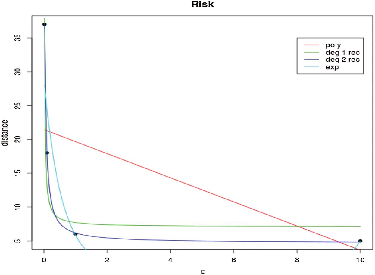
Figure 1: Curve fitting for RoD estimation

Table 1: Predicted RoD and the real RoD

3.3 Evaluating Utility

3.3.1 Baseline Method for Evaluating Utility

As mentioned in the previous sections, even though the synthetic dataset has already achieved the required privacy level, usually the data utility will be sacrificed. So, the objective of data owner is to maximize the data utility subject to the required privacy. Deriving an explicit formulation for privacy and utility is complex; instead, we resort to data-driven approach. A simple idea for deriving the utility is to iteratively generate different synthetic datasets and then determine the corresponding utility. This operation is very time-consuming. In the worst case, one needs an infinite amount of time to try an infinite number of combinations of parameters. As a result, an algorithm capable of efficiently learning the utility of a given synthetic dataset is desired.

The statistics such as the mean, standard deviation, and variance can be seen as the most popular statistics used by the data analysts and so the metrics for evaluating data utility. In what follows, for fair comparison, after the use of synthetic dataset D, we also used these metrics to estimate the error of the result. The error of variance introduced by the synthetic dataset D can be formulated as

ϵAivar=|var(OAi)-var(DAi)|var(OAi)×100%(11)

As a whole, to evaluate the variance error of the entire dataset, what we can do is to sum up the errors for each record,

ϵvar=∑i=1nϵAivar/n.(12)

Obviously, when the synthetic dataset has smaller estimation error, it also leads to better data utility. The analysis of other statistical measures is also consistent to the ones derived from the above formulas. As a result, we used these statistical measures because of the following two reasons. First, it is because of their popularity and simplicity. Second, we can also learn an approximate distribution from these measurements. Moreover, when there are huge errors for these simple statistics, it would definitely lead to catastrophic utility loss for the other complex statistical measures.

3.3.2 Data-Driven Method for Evaluating Utility

Usually, calculating the estimation error from the synthetic dataset is to calculate Eqs. (11) and (12) over the differentially private synthetic datasets with ϵ={0.01,0.1,1,10} is the most straightforward method that we start to try. For example, Fig. 2 where the input dataset is a 5×1e6 health dataset with five attributes HEIGHT, WEIGHT, BMI, DBP, SBP1 shows the errors incurred by different settings of ϵ.

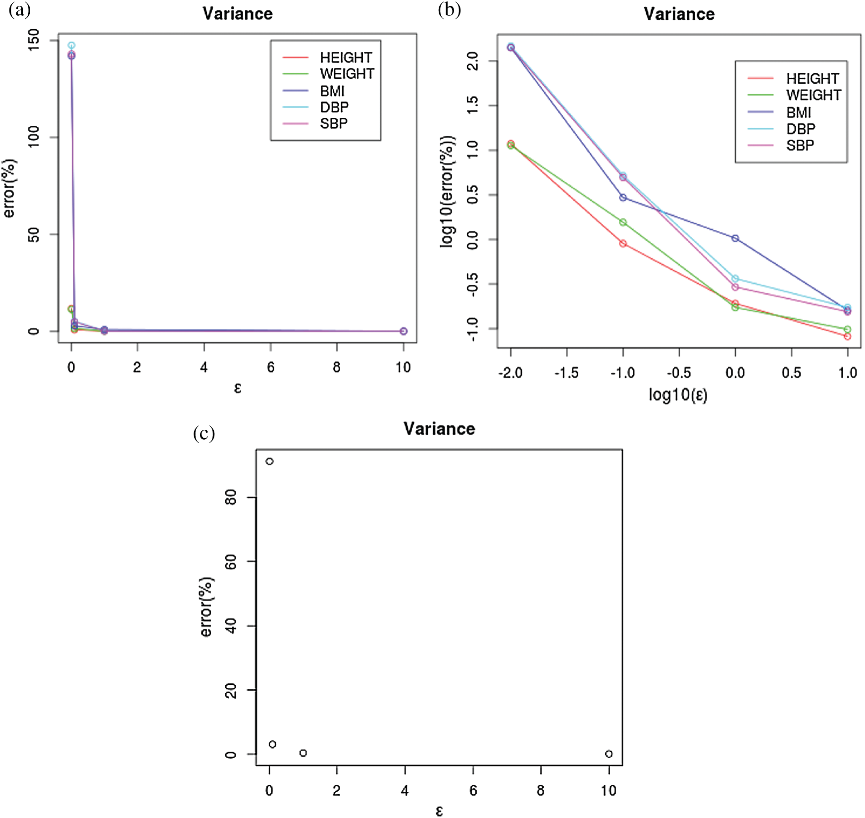
Figure 2: Different methods for the analysis of the error of variance. (a) Each attribute, (b) Log10, (c) average

Iterating the above process of choosing a ϵ, generating a synthetic dataset, and then calculating the utility would be highly inefficient. This is due to the fact that the data owner might want to further improve the utility of the current version of the synthetic dataset. Thus, the data owner will iterate the above process again and again until a satisfactory version appears. As a whole, we decided to generate synthetic datasets for pre-determined ϵ, and then estimate their errors only. After that, our plan is to use these information to fit a curve bridging the privacy and utility. In particular, we propose using a curve fitting, a data-driven approach, as a surrogate method to learn the correlation between ϵ and utility measures such as the error of the mean, standard deviation, and variance. Once we have such a curve from curve fitting, we can indeed calculate ϵ very quickly, given the desired level of utility or vice versa.

Specifically, in the case of ϵvar, ϵvar can be obtained after generating a large number of synthetic datasets with different values of ϵ. Thereafter, the curve could be learned using the obtained values of ϵvar.

However, when performing curve fitting, although this could be used to learn the coefficients that best fit the chosen curve, one factor that we can have freedom to choose is the type of curve. Initially, the two intuitive choices are exponential and polynomial. A more counterintuitive one would be reciprocal curves. We, however, found that the reciprocal curve with the following form:

ϵ^var=aϵ+b,a,b∈R,(13)

where ϵ^var denotes the estimator of ϵvar, leads to the best fit in almost all cases. Here, for completeness, we also present exponential and polynomial curves that correspond to the error of other statistical measures in Fig. 3, in addition to the reciprocal curves. The reciprocal curve fits almost perfectly, as shown in the figure. In our experiments, after averaging all the coefficients from the formulas, we conclude the estimated of ϵvar will be

ϵ^var=15ϵ.(14)

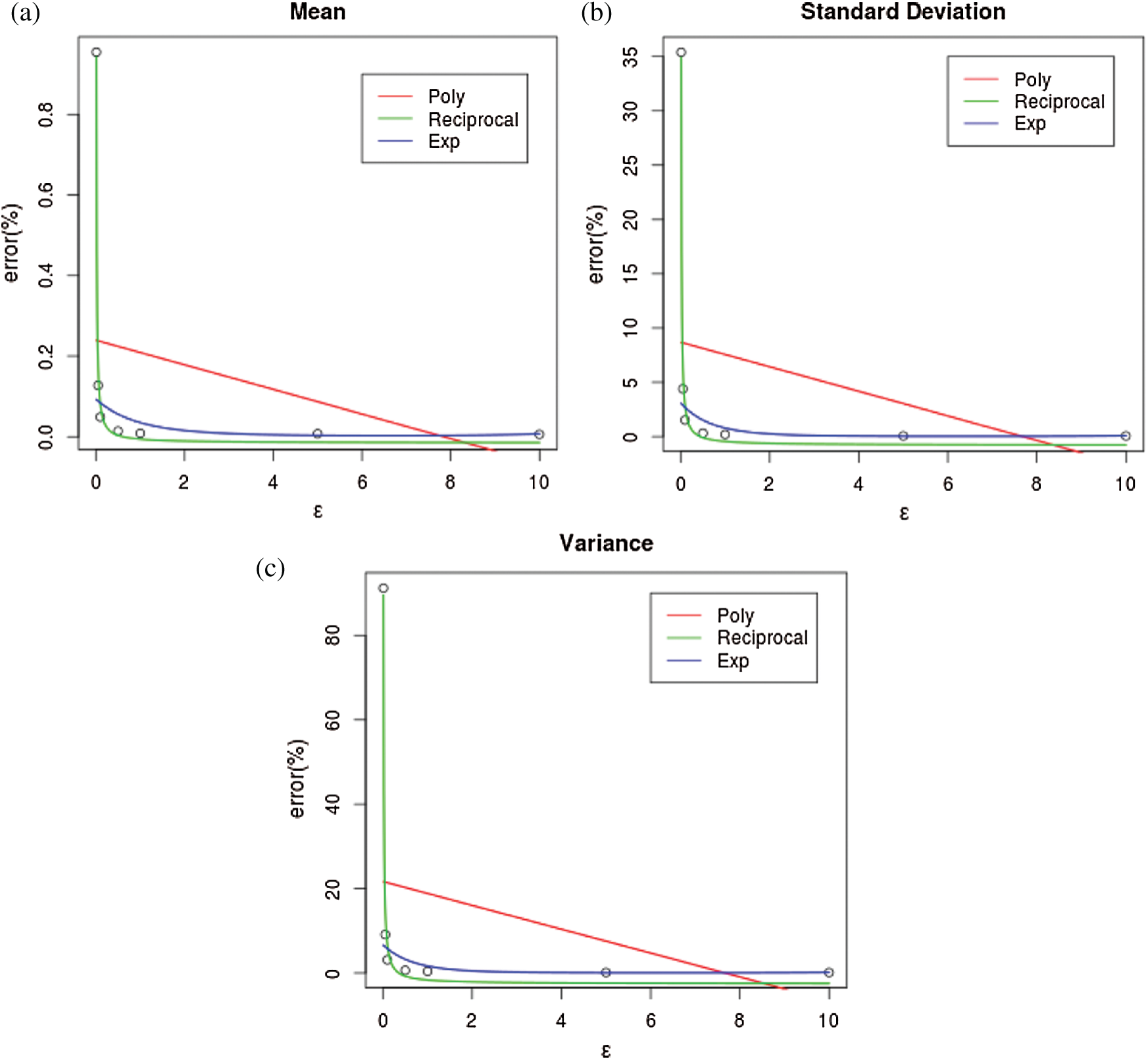
Figure 3: Curve prediction for statistical measures including mean, standard deviation, and variance. (a) Mean (b) standard deviation (c) variance

In fact, Eq. (14) has room to be improved so as to offer better prediction results. In our consideration, we aim to calculate the errors in the cases of ϵ={0.01,0.05,0.1,0.5,1,5,10}. Nevertheless, only three errors are calculated for the cases of ϵ={0.01,0.5,10}. Afterwards, we learn the curve based on these three errors. These results are shown in Fig. 4, where the real statistics and predicted statistics in Tab. 2 are matched almost perfectly.

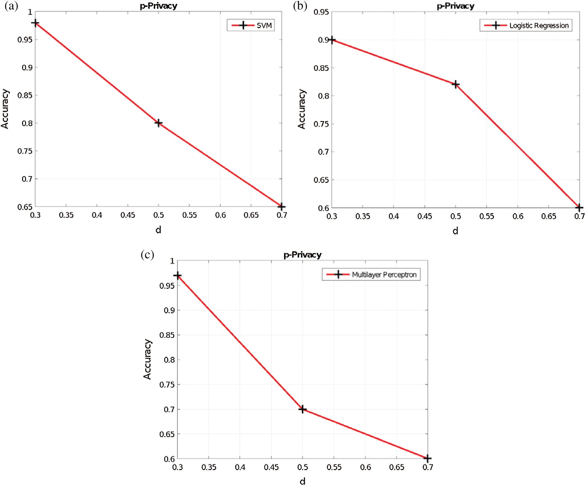
Figure 4: Curve prediction for statistical measures including mean, standard deviation, and variance. (a) Mean (b) Standard deviation (c) variance

Table 2: Comparison between the predicted and real variance errors

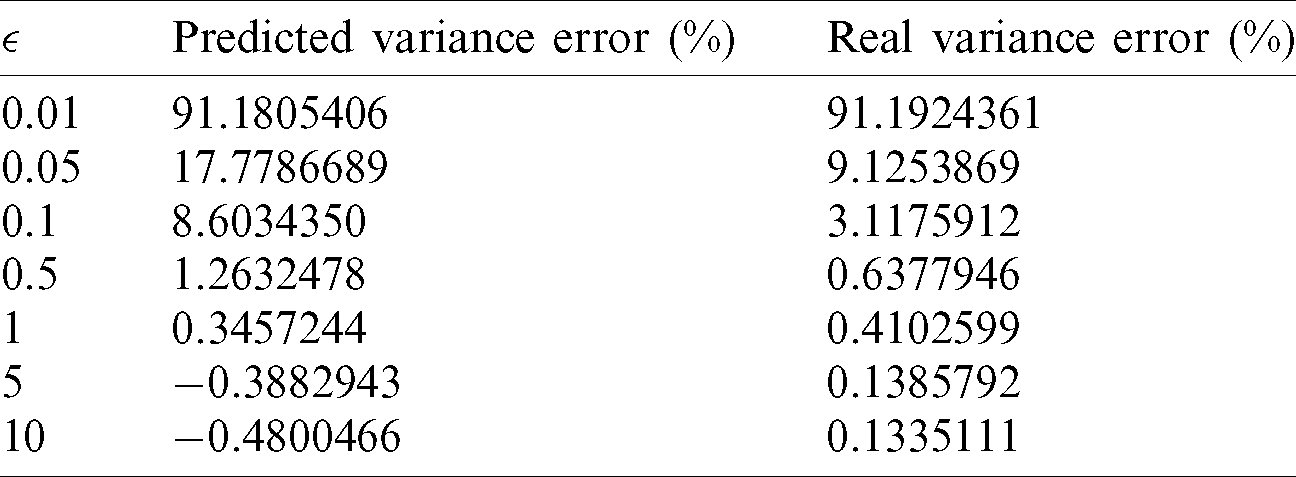
Despite the seemingly satisfactory results in Fig. 4, once we scrutinize Tab. 2, we will find that there are negative predicted values of ϵ={5,10}, and this result is not pleasing. Once fixing the shape of the curve fitting and reciprocal curve, we found that the main reason for predictability degradation of the fitted curve can be attributed to the insufficient degree of the reciprocal (or the other used) curve. Consequently, when we slightly increase the degree of the reciprocal curve, we obtain

ϵ^var=aϵ2+bϵ+c,a,b,c∈R.(15)

Here, after the comparison among the results in both Tab. 3 and Fig. 5, one can know immediately that the predicted errors are matched against the real error values, with a curve newly learned from the data.

Table 3: Comparison of the predicted and real variance errors after applying Eq. (15)

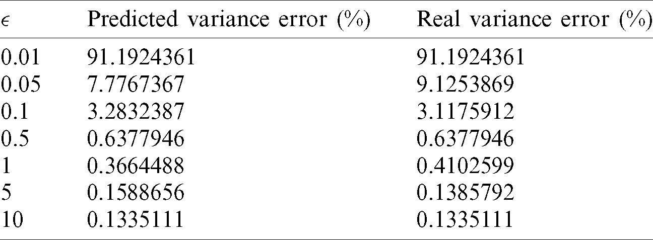
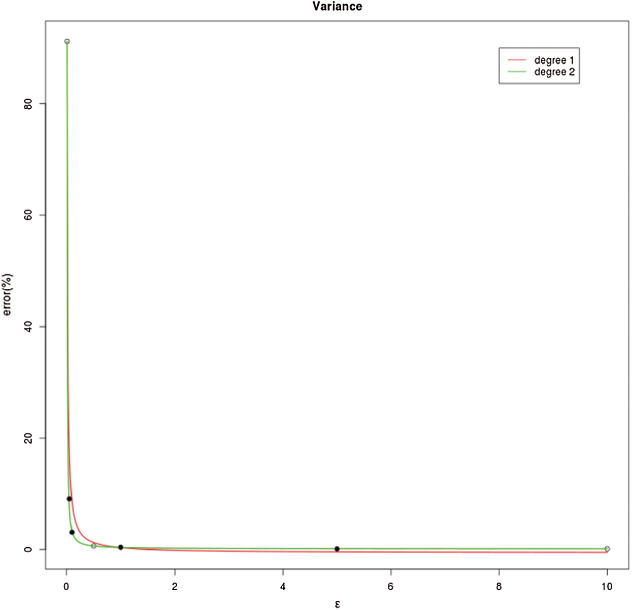
Figure 5: Difference between fitted reciprocal curves with the degree 1 and 2

3.4 Jointly Evaluating RoD and Utility

The data utility results when varying d in the Voronoi privacy, y in the y-privacy, and p in the p-privacy, are provided in Figs. 6–8, respectively. Obviously, as the RoD increases, the data utility is not maintained. This is because additional perturbation is added to the original dataset and therefore the synthetic dataset is generated from a data distribution with more noise.

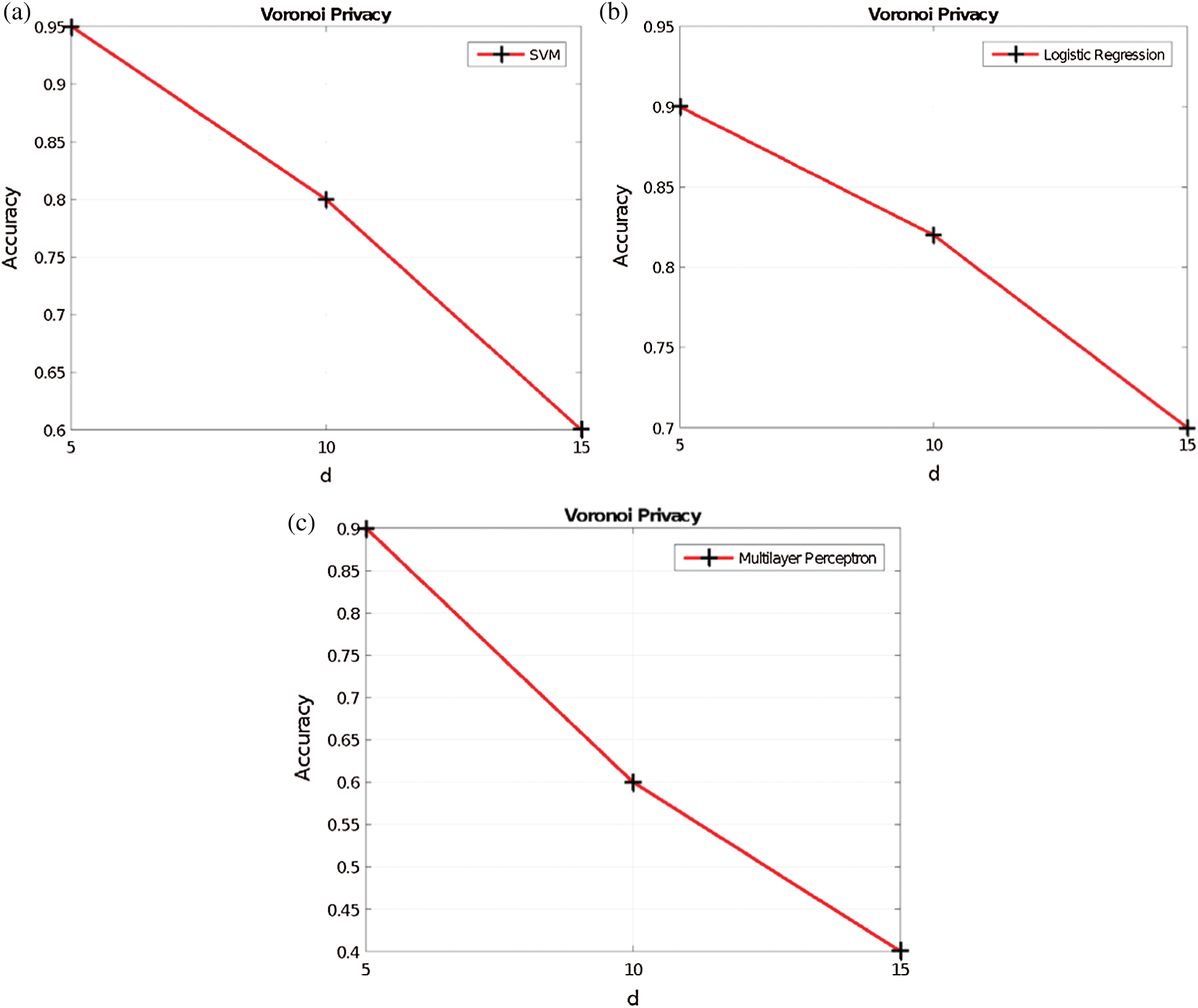
Figure 6: Voronoi privacy vs. accuracy (a) SVM (b) LR (c) MLP

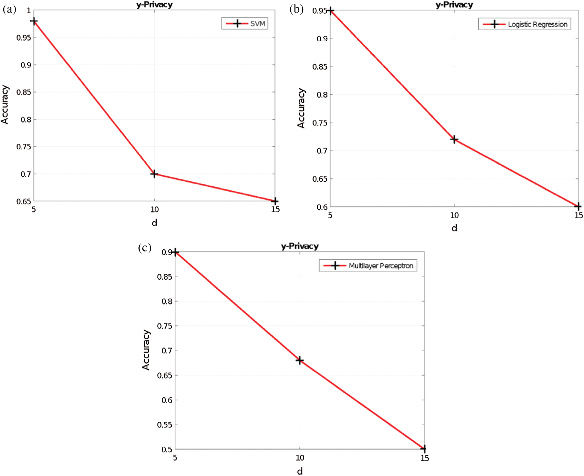
Figure 7: y-privacy vs. accuracy (a) SVM (b) LR (c) MLP

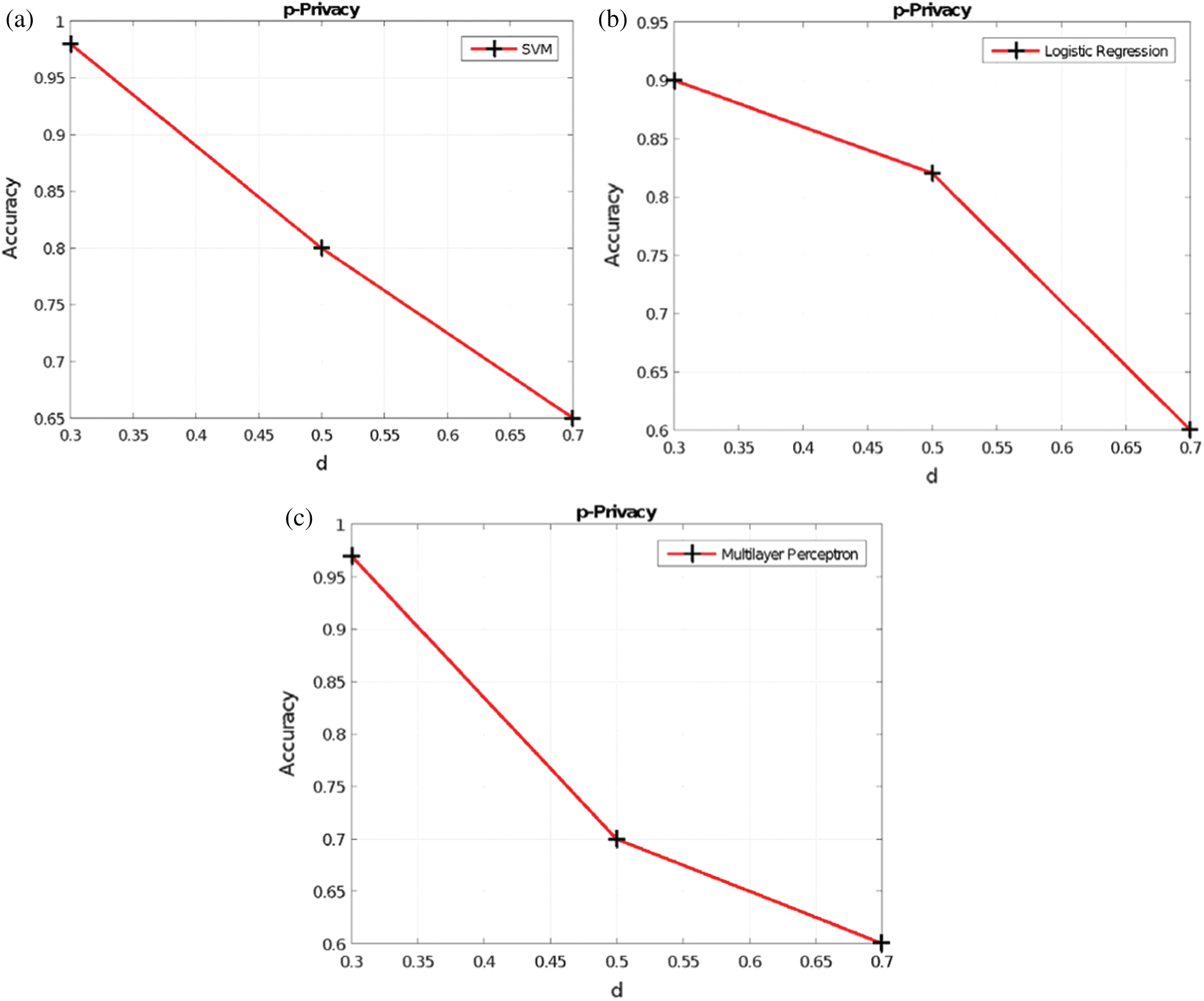
Figure 8: p-privacy vs. accuracy (a) SVM (b) LR (c) MLP

One can know that the extension from the aforementioned data-driven approaches for evaluating both the utility and RoD to a data-driven approach for determining the privacy budget ϵ with a joint consideration of the utility and RoD can be easily achieved. In essence, from Sections 3.2 and 3.3 we will learn different (reciprocal) curves; one for the privacy level and another for utility. While the curves for the privacy and utility are unrelated at the first glance, if we consider the DP definition and the way of how to achieve DP, they, in fact, are correlated to each other. In this sense, multidimensional curve fitting will be an alternative for a more complex setting; i.e., it would be a candidate to be used over the curves learned from Sections 3.2 and 3.3 so as to learn a higher dimensional curve for the privacy level and utility. Since the resulting higher dimensional curve will have a parameter ϵ, after a simple calculation when the other parameters are fixed, the privacy budget ϵ can be determined with a joint consideration of the utility and RoD.

4  Conclusion

In this paper, we proposed a number of friendly privacy notions to measure the RoD. We also developed curve fitting-based approach to determine the privacy budget ϵ in a data-driven manner with the joint consideration of the RoD and utility. This approach enables novice users to grab the idea behind the level of privacy protection and the data utility. As a result, these users would be able to determine an appropriate privacy budget ϵ for DPDR, depending on the amount of privacy risk they would be prepared to tolerate and the desired utility.

Notes

DBP is diastolic blood pressure and SBP is systolic blood pressure. The height and weight are generated by sampling from a normal distribution manually. Meanwhile, the BMI is calculated from the height and weight. Eventually, DBP and SBP are generated from BMI with some noise with small magnitude.

Funding Statement: The work of Chia-Mu Yu has been initiated within the project MOST 110-2636-E-009-018 of Ministry of Science and Technology, Taiwan https://www.most.gov.tw/. Tooska Dargahi is supported by the UK Royal Society Award (Grant Number IEC\R3\183047, https://royalsociety.org/).

Conflicts of Interest: The authors declare that they have no conflicts of interest to report regarding the present study.

References

 1.  B. Marr. (2019). “The Top 5 Fintech Trends Everyone Should Be Watching In 2020,” Forbes, . [Online]. Available: https://www.forbes.com/sites/bernardmarr/2020/12/30/the-top-5-fintech-trends-everyone-should-be-watching-in-2020/?sh=611318a74846. [Google Scholar]

 2.  I. Pollari and A. Ruddenklau. (2020). “Pulse of Fintech H1’20,” Global. KPMG, . [Online]. Available: https://home.kpmg/xx/en/home/insights/2020/09/pulse-of-fintech-h1-20-global.html. [Google Scholar]

 3.  S. Mehrban, M. W. Nadeem, M. Hussain, M. M. Ahmed, O. Hakeem et al. (2020). , “Towards secure FinTech: A survey, taxonomy, and open research challenges,” IEEE Access, vol. 8, pp. 23391–23406. [Google Scholar]

 4.  Data sharing and open data for banks a report for HM treasury and cabinet office,” Open Data Institute, . [Online]. Available: https://assets.publishing.service.gov.uk/government/uploads/system/uploads/attachment_data/file/382273/141202_API_Report_FINAL.PDF. [Google Scholar]

 5.  L. Melrose and M. Clarke. (2020). “The data balancing act a growing tension between protection, sharing and transparency,” Deloitte, . [Online]. Available: https://www2.deloitte.com/pg/en/pages/financial-services/articles/data-balancing-act.html. [Google Scholar]

 6.  C. Duckett. (2017). “Re-identification possible with Australian de-identified Medicare and PBS open dat,” ZDNet, . [Online]. Available: https://www.zdnet.com/article/re-identification-possible-with-australian-de-identified-medicare-and-pbs-open-data/#:. [Google Scholar]

 7.  L. Rocher, J. M. Hendrickx and Y. A. de Montjoye. (2019). “Estimating the success of re-identifications in incomplete datasets using generative models,” Nature Communications, vol. 10, no. 1, pp. 1–9. [Google Scholar]

 8.  D. Barth-Jones. (2012). “The ‘Re-Identification’ of Governor William Weld’s Medical Information: A Critical Re-Examination of Health Data Identification Risks and Privacy Protections, Then and Now,” SSRN Electronic Journal, July. [Google Scholar]

 9.  A. Tanner. (2013). “Harvard professor re-identifies anonymous volunteers in DNA study,” Forbes, . [Online]. Available: https://www.forbes.com/sites/adamtanner/2013/04/25/harvard-professor-re-identifies-anonymous-volunteers-in-dna-study/?sh=41b29ba992c9. [Google Scholar]

10. C. Dwork. (2006). “Differential Privacy,” in Proc. 33rd Int. Colloquium on Automata, Languages and Programming, Venice, Italy. [Google Scholar]

11. N. Mohammed, R. Chen, B. C. Fung and P. S. Yu. (2011). “Differentially private data release for data mining,” in Proc. 7th ACM SIGKDD Int. Conf. on Knowledge Discovery and Data Mining, San Diego, CA. [Google Scholar]

12. L. Sweeney. (2002). “k-anonymity: A model for protecting privacy,” International Journal of Uncertainty, Fuzziness and Knowledge-Based Systems, vol. 10, no. 5, pp. 557–570. [Google Scholar]

13. A. Machanavajjhala, J. Gehrke, D. Kifer and M. Venkitasubramaniam. (2007). “l-diversity: Privacy beyond k-anonymity,” ACM Transactions on Knowledge Discovery from Data, vol. 1, no. 1, pp. 3-es. [Google Scholar]

14. N. Li, T. Li and S. Venkatasubramanian. (2007). “t-closeness: Privacy beyond k-anonymity and l-diversity,” in Proc. IEEE 23rd Int. Conf. on Data Engineering, Istanbul, Turkey. [Google Scholar]

15. Disclosure Avoidance and the 2020 Census. (2020). “United States Census Bureau,” . [Online]. Available: census.gov/about/policies/privacy/statistical_safeguards/disclosure-avoidance-2020-census.html. [Google Scholar]

16. J. Zhang, G. Cormode, C. M. Procopiuc, D. Srivastava and X. Xiao. (2017). “Privbayes: Private data release via bayesian networks,” ACM Transactions on Database Systems, vol. 42, no. 4, pp. 1–41. [Google Scholar]

17. D. McClure and J. P. Reiter. (2012). “Differential privacy and statistical disclosure risk measures: An investigation with binary synthetic data,” Transactions on Data Privacy, vol. 5, pp. 535–552. [Google Scholar]

18. R. Torkzadehmahani, P. Kairouz and B. Paten. (2019). “DP-CGAN: Differentially private synthetic data and label generation,” in Proc. IEEE Conf. on Computer Vision and Pattern Recognition Workshops, Long Beach, CA. [Google Scholar]

19. B. K. Beaulieu-Jones, Z. S. Wu, C. Williams, R. Lee, S. P. Bhavnani et al. (2019). , “Privacy-preserving generative deep neural networks support clinical data sharing,” Circulation: Cardiovascular Quality and Outcomes, vol. 12, no. 7. [Google Scholar]

20. L. Xie, K. Lin, S. Wang, F. Wang and J. Zhou. (2018). “Differentially private generative adversarial network,” arXiv preprint arXiv: 1802.06739. [Google Scholar]

21. C. Xu, J. Ren, D. Zhang, Y. Zhang, Z. Qin et al. (2019). , “GANobfuscator: Mitigating information leakage under gan via differential privacy,” IEEE Transactions on Information Forensics and Security, vol. 14, no. 9, pp. 2358–2371. [Google Scholar]

22. J. Jordon, J. Yoon and M. van der Schaar. (2018). “PATE-GAN: Generating synthetic data with differential privacy guarantees,” in Proc. Int. Conf. on Learning Representations, Vancouver, Canada. [Google Scholar]

23. W. Qardaji, W. Yang and N. Li. (2014). “PriView: practical differentially private release of marginal contingency tables,” in Proc. of the 2014 ACM SIGMOD Int. Conf. on Management of Data, Snowbird, Utah. [Google Scholar]

24. H. Li, L. Xiong, L. Zhang and X. Jiang. (2014). “DPSynthesizer: Differentially private data synthesizer for privacy preserving data sharing,” in Proc. of the VLDB Endowment Int. Conf. on Very Large Data Bases, Hangzhou, China. [Google Scholar]

25. Y. Xiao, J. Gardner and L. Xiong. (2012). “DPCube: Releasing differentially private data cubes for health information,” in Proc. of the IEEE 28th Int. Conf. on Data Engineering, Dallas, Texas. [Google Scholar]

26. H. Li, L. Xiong and X. Jiang. (2014). “Differentially private synthesization of multi-dimensional data using copula functions,” in Proc. of the Int. Conf. on Advances in Database Technology, Athens, Greece. [Google Scholar]

27. X. Xiao, G. Wang and J. Gehrke. (2010). “Differential privacy via wavelet transforms,” IEEE Transactions on Knowledge and Data Engineering, vol. 23, no. 8, pp. 1200–1214. [Google Scholar]

28. J. Lee and C. Clifton. (2011). “How much is enough? Choosing ϵ for differential privacy,” in Proc. Int. Conf. on Information Security, Xi’an, China. [Google Scholar]

29. J. Hsu, M. Gaboardi, A. Haeberlen, S. Khanna, A. Narayan et al. (2014). , “Differential Privacy: An economic method for choosing epsilon,” in Proc. of the IEEE 27th Computer Security Foundations Symp., Vienna, Austria. [Google Scholar]

30. M. Naldi and G. D’Acquisto. (2015). “Differential privacy: An estimation theory-based method for choosing epsilon,” arXiv preprint arXiv:1510.00917. [Google Scholar]

31. Y. T. Tsou, H. L. Chen and Y. H. Chang. (2019). “RoD: Evaluating the risk of data disclosure using noise estimation for differential privacy,” IEEE Transactions on Big Data. [Google Scholar]

32. R. Sarathy and K. Muralidhar. (2011). “Evaluating laplace noise addition to satisfy differential privacy for numeric data,” Transaction on Data Privacy, vol. 4, no. 1, pp. 1–17. [Google Scholar]

33. C. Dwork, F. McSherry, K. Nissim and A. Smith. (2006). “Calibrating noise to sensitivity in private data analysis,” in Proc. Theory of Cryptography Conf., New York, NY. [Google Scholar]

34. F. Aurenhammer. (1991). “Voronoi diagrams—a survey of a fundamental geometric data structure,” ACM Computing Surveys, vol. 23, no. 3, pp. 345–405. [Google Scholar]

35. B. Kalantari. (2013). “The State of the Art of Voronoi Diagram Research,” Transactions on Computational Science, vol. 8110, pp. 1–4. [Google Scholar]

36. H. Long, S. Zhang, J. Wang, C.-K. Lin and J.-J. Cheng. (2017). “Privacy preserving method based on Voronoi diagram in mobile crowd computing,” International Journal of Distributed Sensor Networks, vol. 13, no. 10, pp. 155014771773915. [Google Scholar]

37. S. Takagi, Y. Cao, Y. Asano and M. Yoshikawa. (2019). “Geo-graph-indistinguishability: Protecting location privacy for LBS over road networks,” in Proc. IFIP Annual Conf. on Data and Applications Security and Privacy, Charleston, South Carolina. [Google Scholar]

38. M. Bi, Y. Wang, Z. Cai and X. Tong. (2020). “A privacy-preserving mechanism based on local differential privacy in edge computing,” China Communications, vol. 17, no. 9, pp. 50–65. [Google Scholar]

39. F. Aurenhammer, R. Klein and D.-T. Lee. (2013). Voronoi Diagrams and Delaunay Triangulations, Singapore: World Scientific Publishing Company. [Google Scholar]

40. R. A. Dwyer. (1991). “Higher-dimensional voronoi diagrams in linear expected time,” Discrete & Computational Geometry, vol. 6, no. 3, pp. 343–367. [Google Scholar]

41. S. Arya and T. Malamatos. (2002). “Linear-size approximate voronoi diagrams,” in Proc. the Thirteenth Annual ACM-SIAM Symp. on Discrete Algorithms, Philadelphia, PA. [Google Scholar]

42. R. Chen, Q. Xiao, Y. Zhang and J. Xu. (2015). “Differentially private high-dimensional data publication via sampling-based inference,” in Proc. the 21th ACM SIGKDD Int. Conf. on Knowledge Discovery and Data Mining, Sydney, Australia. [Google Scholar]

This work is licensed under a Creative Commons Attribution 4.0 International License, which permits unrestricted use, distribution, and reproduction in any medium, provided the original work is properly cited.