DOI:10.32604/cmc.2021.015318
| Computers, Materials & Continua DOI:10.32604/cmc.2021.015318 | |
| Article |
An Optimized Deep Residual Network with a Depth Concatenated Block for Handwritten Characters Classification
Department of Information Systems, King Abdulaziz University, Jeddah, 21589, SA
*Corresponding Author: Gibrael Abosamra. Email: gabosamra@kau.edu.sa
Received: 15 November 2020; Accepted: 24 December 2020
Abstract: Even though much advancements have been achieved with regards to the recognition of handwritten characters, researchers still face difficulties with the handwritten character recognition problem, especially with the advent of new datasets like the Extended Modified National Institute of Standards and Technology dataset (EMNIST). The EMNIST dataset represents a challenge for both machine-learning and deep-learning techniques due to inter-class similarity and intra-class variability. Inter-class similarity exists because of the similarity between the shapes of certain characters in the dataset. The presence of intra-class variability is mainly due to different shapes written by different writers for the same character. In this research, we have optimized a deep residual network to achieve higher accuracy vs. the published state-of-the-art results. This approach is mainly based on the prebuilt deep residual network model ResNet18, whose architecture has been enhanced by using the optimal number of residual blocks and the optimal size of the receptive field of the first convolutional filter, the replacement of the first max-pooling filter by an average pooling filter, and the addition of a drop-out layer before the fully connected layer. A distinctive modification has been introduced by replacing the final addition layer with a depth concatenation layer, which resulted in a novel deep architecture having higher accuracy vs. the pure residual architecture. Moreover, the dataset images’ sizes have been adjusted to optimize their visibility in the network. Finally, by tuning the training hyperparameters and using rotation and shear augmentations, the proposed model outperformed the state-of-the-art models by achieving average accuracies of 95.91% and 90.90% for the Letters and Balanced dataset sections, respectively. Furthermore, the average accuracies were improved to 95.98% and 91.06% for the Letters and Balanced sections, respectively, by using a group of 5 instances of the trained models and averaging the output class probabilities.
Keywords: Handwritten character classification; deep convolutional neural networks; residual networks; GoogLeNet; ResNet18; DenseNet; drop-out; L2 regularization factor; learning rate
Handwritten character recognition has a wide spectrum of applications in all software systems that allow handwritten input through an electronic stylus or digital tablet or through an offline scan of documents such as postal envelopes, bank cheques, medical reports, or industrial labor reports. The handwritten alphanumeric character recognition problem is still a challenge in the field of pattern recognition due to the high variability within each handwritten class and the high similarity among certain classes in the alphabet itself. The EMNIST dataset [1] is considered one of the recent datasets that possess such difficulties where there is variability within each class due to the variability of the patterns produced by different writers and variability for the same writer who produces different patterns for the same character due to the nature of the handwriting process itself. Traditional machine-learning techniques have been developed to tackle this challenge, leading to accuracies that may be accepted for old datasets such as the Modified National Institute of Standards and Technology dataset (MNIST). Recently deep-learning techniques, especially Deep Convolutional Neural Networks (DCNN), made a breakthrough that upgrades the recognition accuracy of machines to an accuracy level comparable to a human being’s recognition accuracy. The MNIST dataset is now considered an already solved problem where the percentage error of many works approaches 0.2% that is considered to be irreducible. The EMNIST dataset is built to represent the new challenging handwriting alphanumeric dataset instead of the old MNIST dataset. The EMNIST is an extended version of the MNIST dataset [2], which consists of 52 characters (both upper and lowercase) and 10 digits. It includes a total of 814255 samples from almost 3700 writers [1]. The dataset has different labeling schemas: (1) By_class (62 alphanumeric characters: digits: 0–9, upper case: A–Z, and lower case: a–z), (2) By_merge (47 classes: digits 0–9, 37 fused upper and lower case letters where similar upper and lower letters are unified), (3) Letters (26 classes having one class for each letter, either upper or lower), and (4) Digits (10 classes: 0–9 with more and different samples than MNIST digits). A Balanced dataset section is introduced that represents a reduced version of the By_merge section but has an equal number of samples for each label. A limited number of systems have been built to reach significant classification accuracies of the different sections of the EMNIST dataset, as will be shown in Section 2.
Our approach is mainly based on starting with the architectures of two main ready-made image classification DCNN models and modify them by exploring the possible dimensions of variations such as increasing or decreasing the number of building blocks (or layers) to select the faster and more accurate one, and then enhance the selected architecture. Also, the suitable pre-processing and augmentation of the image data is accompanied to get the highest possible accuracy to compete with state-of-the-art results.
In Section 2, we summarize and record the state-of-the-art results of the most important researches done on the Letters and Balanced sections of the EMNIST dataset. In Section 3, a brief background of DCNN and the smallest DCNN models that we think have significant achievement in the image classification problem is presented. In Section 4, our work is elaborated with detailed experiments, in addition to the presentation of the different types of image preprocessing and data augmentation that are considered, until reaching a final configuration of a DCNN that gives competing accuracy with state-of-the-art systems. In Section 5, final experiments are performed on the Letters and Balanced sections of the dataset, and two extra experiments are performed on each section using a reduced training set for each dataset section. In Section 6, our work is compared with state-of-the-art works. Finally, important contributions are summarized in the conclusions and future work section.
In this section, we concentrate on CNN, Capsule network (CapsNet), and machine-learning based efforts done after the creation of the EMNIST dataset [1]. Works done on the National Institute of Standards and Technology dataset (NIST) Special Database 19 (from which EMNIST was obtained) can be found in [3]. Also, we mainly refer to works done on the Letters and Balanced sections only.
The authors of the original EMNIST paper [1] included a baseline using a linear classifier and the Online Pseudo-Inverse Update Method (OPIUM) [4]. Using OPIUM, the highest baseline reported accuracies were 85.15% for the Letters dataset and 78.02% for the Balanced dataset.
The authors of [5] combined Markov random field-models with CNN (MRF-CNN) for image classification. They reported accuracies of 95.44% and 90.29% when applying their technique to the Letters and Balanced datasets, respectively.
The authors of [6] used K-Nearest Neighbor (KNN) and Support Vector Machine (SVM) classifiers to classify handwritten characters based on features extracted by a hybrid of Discrete Wavelet Transform (DWT) and Discrete Cosine Transform (DCT). They reported accuracy of 89.51% when their model was applied to the Letters data set (using SVM based on DWT’s and DCT’s combined features).
In [7], a bidirectional neural network (BDNN) was designed to perform both image recognition and reconstruction using an added style memory to the output layer of the network. When their model was tested on the EMNIST Letters dataset, it achieved an accuracy of 91.27%.
Some authors have made use of neural architecture searches to automatically optimize the hyper parameters of CNN classifiers. For example, Dufourq et al. [8] introduced a technique called Evolutionary Deep Networks for Efficient Machine Learning (EDEN). They applied neuro evolution to develop CNN networks for different classification tasks achieving an accuracy of 88.3% with the EMNIST Balanced dataset. Researchers in [9] used genetic algorithms in the automatic design of DCNN architectures (Genetic DCNN) for new image classification problems. When their generated architecture was applied to the Letters dataset, it achieved an accuracy of 95.58%, which is the highest published accuracy to date.
Committees of neuro evolved CNNs using topology transfer learning have been introduced by the authors [10], who obtained an accuracy of 95.35% with the EMNIST Letters dataset. Due to the highly challenging level of this classification task, they resorted to the use of 20 models to enhance accuracy from 95.19% to 95.35% which was still less than the highest previously recorded accuracy (95.44%).
Researchers [11] introduced a hierarchical classifier that uses automatic verification based on a confusion matrix extracted by a regular (flat) classifier to enhance the accuracy of a specific classifier type. It relatively succeeded in enhancing the accuracy of some machine-learning based techniques such as the linear regression classifier but not in enhancing the accuracy of the CNN classifier. Its flat CNN classifier resulted in an accuracy of 93.63% and 90.18% when applied to the Letters and Balanced datasets, respectively.
The researchers [12] proposed TextCaps, which used two capsule layers (a highly advanced concept introduced by Sabour et al. [13]) preceded by 3 CNN layers. They reported accuracies of 95.36% and 90.46% for EMNIST Letters and EMNIST Balanced datasets, respectively.
Some researchers designed DCNN architectures to classify letter sets other than the English alphanumeric handwritten characters and then tested their models in the EMNIST database. For example, the researchers [14] built a DCNN for the classification of Arabic letters, and when they tested their architecture on the EMNIST Letters dataset, they reported accuracy of 95%. Similarly, the authors of [15] designed a system using a DCNN with six CNN layers and two fully connected layers for Bangla handwritten digit recognition. They reported an accuracy of 90.59% when their DCNN model was tested on the EMNIST Balanced dataset. Fig. 1 displays a timeline of the accuracy recorded for the Letters dataset in the mentioned references based on their published dates.
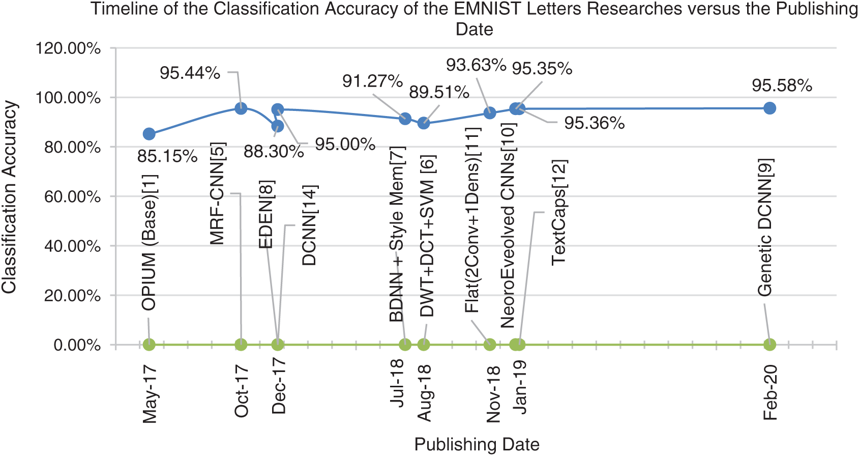
Figure 1: A timeline graph of the accuracies achieved by different researches on the Letters dataset
From Fig. 1, it is clear that DCNN-based techniques resulted in higher accuracies compared with machine-learning techniques or non-deep learning techniques when applied to the EMNIST Letters dataset. Also, some techniques more advanced than DCNN did not achieve remarkable accuracies such as the CapsNet (TextCaps [12]) although characterized by orientation-invariability and requires less number of training samples.
From the timeline curve, we also observe two global peaks. The first significant peak was achieved in October 2017 by the MRF-CNN technique [5] with a 10.29% increase from the base classifier [1]. All subsequent works from October 2017 until February 2020 didn’t even reach the achieved accuracy of 95.44% (in October 2017). The second peak (95.58%) was achieved after approximately two-and-a-half years by the Genetic DCNN technique [9], which raised accuracy by 0.14%.
The timeline includes two very close local peaks (there is mathematically one peak, but because their accuracies are very close we can consider them two in one) representing two highly advanced techniques ([10,12] published on 1 January 2019 and 9 January 2019, respectively), which have a 0.01% difference in accuracy.
The same conclusions are drawn when investigating the achievements in the case of the Balanced dataset, but with lower accuracy due to the inclusion of more classes (47) than the Letters dataset (26 classes), which resulted in more confusing letter shapes.
An important conclusion to be drawn from this review is that no advanced architecture of the DCNN [16] (such as ResNet, Inception, DenseNet) has been applied to the EMNIST Letters or Balanced datasets in standalone research. The researchers [9] tested some ready-made architectures without modifications on the EMNIST letters yielding accuracies of 89.36%, 94.62%, and 94.44% using AlexNet, VGGNet, and ResNet, respectively. Hence, in this paper, we will introduce standalone research to optimize one of these advanced architectures, specifically the ResNet architecture, to achieve higher classification scores on the Letters and Balanced datasets.
3 Review of the Concerned Convolutional Networks
In this section, we summarize the basic building blocks of DCNN and the two most famous DCNN networks, mainly GoogLeNet and ResNet18 and the main concepts on which these networks are based, in addition to a brief definition of the drop-out technique.
3.1 Deep Convolutional Neural Networks (DCNNs)
A typical DCNN is composed of many convolutional layers, max-pooling layer and/or average-pooling layers, one or two fully connected layers and finally a softmax layer in the case of classification tasks. The purpose of a convolutional layer is to map an M-channel Input (image) of size
As described in the previous subsection, in a convolutional operation at one location, every output channel (N) is connected to every input channel (M), so it is called a dense connection architecture. The GoogLeNet [17] builds on the idea that most of the activations in a deep network are either unnecessary (value of zero) or redundant because of correlations between them. Therefore, the most efficient architecture of a deep network will have a sparse connection between the input and output activations, which implies that all N output channels (FMs) will not have a connection with all the M input channels (FMs). There are techniques to prune out such connections which would result in a sparse weight/connection. However, kernels for sparse matrix multiplication are not optimized in libraries such as BLAS or CuBlas (CUDA for GPU) packages, which render them even slower than their dense counterparts. So, GoogLeNet devised an inception module that approximates a sparse CNN with a normal dense construction (as shown in Fig. 3).
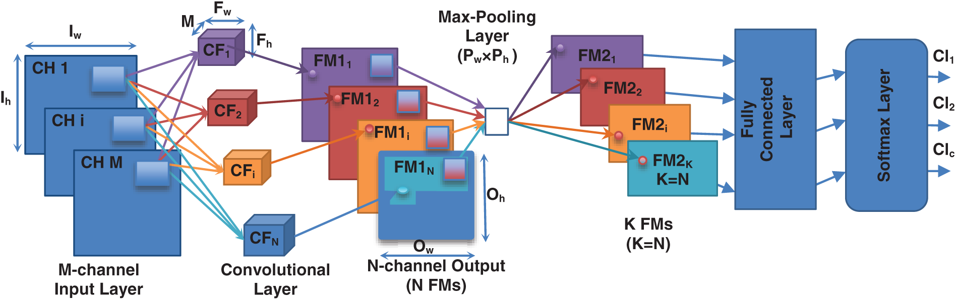
Figure 2: A simple DCNN composed of an input layer, a convolutional layer, a max-pooling layer, a fully connected layer, and a softmax layer
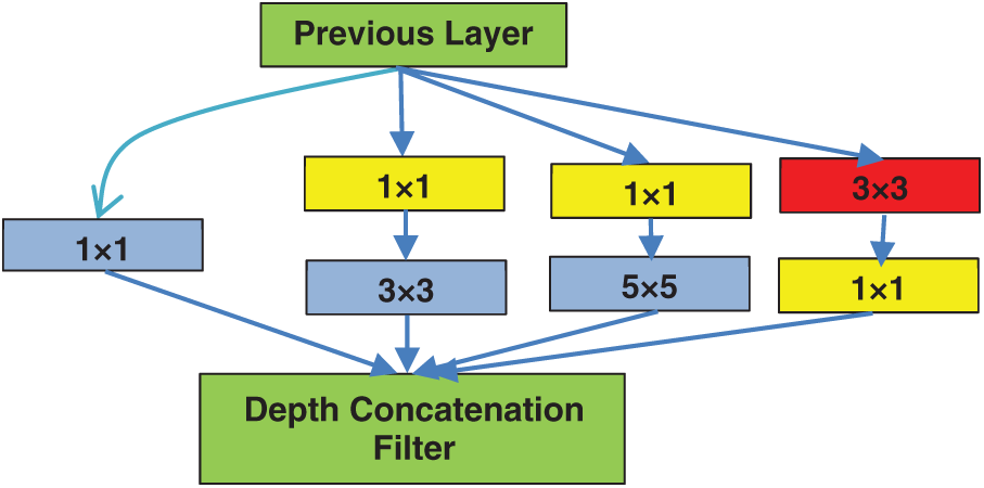
Figure 3: Inception module with dimension reduction using
Since only a small number of neurons are effective as mentioned earlier, the width/number of the CFs of a particular kernel size is kept small. Also, it uses convolutions of different sizes to capture details at different scales (
Another salient point about the inception module is that it has a so-called bottleneck layer (
The GoogLeNet model is built of 9 inception modules in addition to the lower layers of traditional convolution and max pooling and the final layers for average pooling, drop-out, linear mapping (fully connected), and soft-max layer for classification. All the convolutions, including those inside the inception modules, use rectified linear activation. By running multiple instances of the GoogleNet in conjunction with several types of data augmentation and by aggregation of their class probability outputs, the GoogleNet team achieved a top-5 error of 6.67% in the ILSVRC 2014 competition.
Residual networks are deep networks that solve the degradation problem by letting a layer or group of layers learn the residual of a mapping function instead of learning the complete mapping function by making the output mapping equal to the summation of the input plus the learned function [18]. In other words, if we assume that the input is a simple variable X and the output is the required mapping MP(X), the learned function F(X) will be
This is accomplished simply by using a direct shortcut connection from the input and adding it to the output as shown in Fig. 4, which includes two mapping layers, each followed by a Rectified Linear Unit (ReLU).
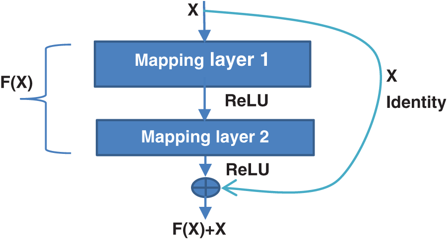
Figure 4: A basic residual learning building module (or block) [18]
When N residual modules are cascaded, the final residual output ResOut(N) without regarding the intermediate non-linear effects can be defined iteratively by the following formula:
where
Which can be represented by the following recursive formula:
where FN is the learned function at block N.
A very important characteristic of residual networks that makes them compete with inception networks is that a residual network that includes many residual modules with intermediate down sampling between every two modules has the advantage of combining different scales of the input image using addition in an iterative manner rather than combining them using concatenation in a parallel manner in the inception networks. Thus, the residual architecture allowed deeper networks (such as ResNet18) to learn better than plain networks and hence achieved higher accuracies on many well-known datasets such as ImageNet and CIFAR-10 than previous plain networks [18]. The ResNet18 model is built of 8 residual modules preceded by lower layers of traditional convolution and max-pooling and followed with final layers for average pooling, linear mapping (fully connected), and a soft-max layer for classification. Batch normalization [19] is adapted right after each convolution and before rectified linear activation.
Overfitting is a serious problem in a deep neural network, especially when a large set of parameters is used to fit a small set of training data. Drop-out is a powerful technique to address this issue [20]. This works by randomly removing neurons at a fixed probability during training, and then using a whole architecture at test time. This counts as combining different “thinned” subnets for improving the performance of the overall architecture. Drop-out is used in GoogLeNet, while it is not used in ResNet18. We will add a drop-out layer in the residual DCNN solution to test its effect on classification accuracy.
4 Development of the Proposed Solution Through Experimentation
In this section, we start implementing our methodology by experimenting and comparing the two lightweight prebuilt models GoogLeNet and ResNet18 in the classification of the EMNIST Letters dataset with demonstration of important types of image preprocessing and data augmentation methods that can help in increasing classification accuracy.
Then, the architectures of both models (ResNet18 and GoogLeNet) are modified by the removal or the addition of a limited number of their basic building blocks, and the effects of the modifications are tested based on the resultant accuracy.
Finally, fine-tuning of the selected architecture from the previous step is achieved through some architecture modifications such as the insertion of a drop-out layer (with proper drop-out probability) and the replacement of one or more addition layers with depth concatenation layer(s), in addition to the selection of the best augmentation methods and the optimum values for the training hyper parameters such as learning rate and regularization factor. It is important to note that due to the stochasticity involved in the training process, every experiment is repeated three times, and the mean accuracy of the three generated models is used to identify the best architecture modification or parameter value that will be implemented in the final solution(s). Only the final solutions are repeated fifteen times, and their mean accuracies are calculated and recorded for comparison with state-of-the-art results. Since we have based our methodology on using a pre-built DCNN that has already been optimized for recognizing images and our goal is to adapt this architecture to recognize handwritten character images, we use a concept similar to partial differentiation by changing a single parameter and observing its effect and using the best one or two values for this parameter and continue in this manner using a beam search with a beam width of two in most cases until reaching to optimal or semi-optimal tuning of the used architecture. The reason for using a beamwidth of two is that the tested parameters may have a correlation and also due to the stochasticity of the training process. Increasing the beam width to 3 or 4 may be necessary in some cases to guarantee that we didn’t miss a significant solution path, especially when there is a structural modification such as adding (or removing) layers (or blocks) or changing the way of merging two layers from addition to concatenation. Also, using a beamwidth of 1 is possible if the best path is very clear.
4.1 Preprocessing and Data Augmentation
Although, the dataset images are well prepared, some preprocessing may be needed to enhance the visibility of the images to the deep network model used in this research. Also, the adaption of the input images to the required input characteristics of these models such as resizing and gray-to-color conversion is performed whenever necessary.
4.1.1 Increasing the Background Area Around the Bodies of the Characters
Although the bodies of the characters are centered in the images of the characters of the EMNIST dataset, some character bodies may extend to touch the end of the boundary of their images. Increasing the background area (surrounding blank pixels) around the bodies of the characters allows the bodies of the characters (or their transformed versions) to be processed by the CFs without being affected by the padding mechanism needed at the boundary of the images, either in the earlier layers of the network or the deeper layers. In addition, during image augmentations such as rotation, the resultant images may suffer from distortion if the rotated size of the character body exceeds the original image size.
Increasing the background area around the bodies of the characters minimizes such effects. For example, if the character body is represented by zeros and the background by ones and the character stroke touches the extreme ends of the rectangle surrounding the character, then zero padding will increase the thickness of the character stroke by the amount of padding.
By adding a blank padding of 6 pixels per side (for example), the character image size becomes
4.1.2 Image Resizing and Gray-to-Color Conversion
Image resizing is done using bi-cubic interpolation [21]. Grey-to-color conversion is done simply by using three copies of each grey image to represent the three channels of the color version to adapt the image with the input characteristics of the used network model. This type of conversion is needed only when training the original model with its pre-trained parameters on the new images dataset in a transfer-learning paradigm.
Although, the number of training samples in each EMNIST dataset section is large, some type of data augmentation is needed to increase the trained model generalization when subjected to new unseen samples in the testing phase.
Since we deal with handwritten characters, image rotation and shearing [22] are beneficial augmentation methods because they increase the possible views of the input data and hence increase the network ability for generalization, as will be shown in the early and fine-tuning experiments.
4.2 Testing ResNet18 and GoogLeNet
In this subsection, GoogLeNet and ResNet18 prebuilt DCNN models are tested through transfer learning on the EMNIST Letters dataset. The models are used in two cases with and without their pre-trained weights.
Since these prebuilt networks were built to classify color images with different sizes, the Letters dataset images are resized, and each image is copied 3 times to represent the 3-channel images to be compatible with the required input of the concerned DCNN model. In the case of using the models without their pre-trained weights, the inputs of the models are modified to accept 1-channel images, as will be done in the following subsections.
This model accepts 3-channel images with a size of
Training of the modified net is done using Stochastic Gradient Descent with Momentum (SGDM) optimizer [23] with a base learning rate of 0.1 and learning rate drop factor of 0.1 applied every 6 epochs for a total number of 30 epochs.
It is worth mentioning that all network training is done using SGDM optimizer, unless stated explicitly otherwise. The mini-batch size is 128 samples per iteration. Shuffling is done randomly every epoch to change the order of the image samples during training in order to minimize overfitting and decrease the probability of getting stuck in local minima [24]. The default regularization factor value (0.0001) is used until its optimum value is determined in different configurations. The default momentum value of 0.9 is used whenever the SGDM optimizer is used.
This experiment resulted in 95.06% classification accuracy. For instance, when the ResNet18 model has been modified to accept
This model accepts images with the same characteristics as ResNet18, and the images are resized and prepared in the same way mentioned in the previous subsection. Also, the last two layers are replaced with new ones to support 26 classes instead of 1000 classes.
The SGDM optimizer is also used, just as in the previous experiment, but with a base learning rate of 0.001. This experiment resulted in 95.37% classification accuracy.
4.2.3 Testing the Effects of the Selected Pre-Processing and Image Augmentation Methods
In this subsection, the previous two experiments with ResNet18 and GoogLeNet are performed in different situations with the original networks without loading the pre-trained parameters using gray input images (or 1-channel images). In the case of GoogLeNet, Adaptive Moment Estimation (ADAM) learning algorithm [25] is used with a base learning rate of 0.0001 in case of 1-channel images because of convergence problems. In addition, the images are inverted. The effect of extra blank padding around the original character images (as stated in the previous section, where the character images are padded with 6-pixels in the four sides to get a
Table 1: The accuracies of the single and 3-channel versions of the GoogLeNet and ResNet18 when applied to the EMNIST Letters dataset section under different blank-padding and augmentation conditions
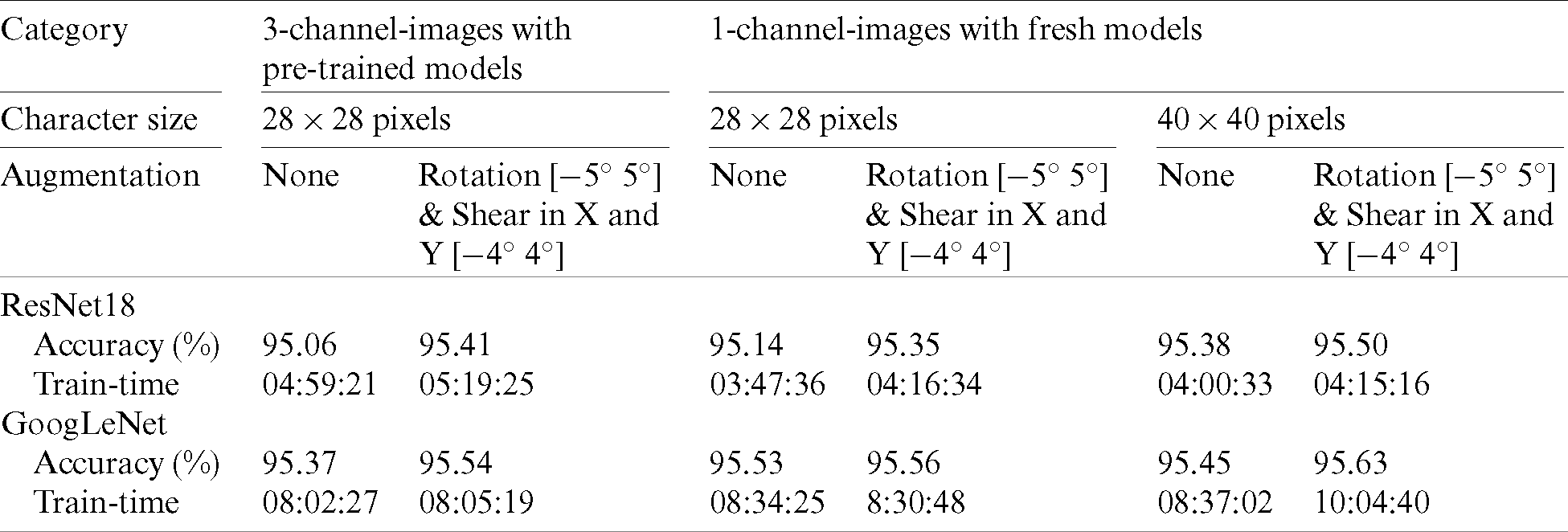
The experiments are conducted on a desktop computer that is equipped with a Windows 10 Pro operating system, 16 GB random-access memory (RAM), Intel core i7-8700K CPU@3.70 GHz and a graphical accelerated processing unit (GPU) of NVIDIA GeForce GTX 1080 Ti with 11 GB RAM. All experiments are programmed using MATLAB 2019A, and some of the later experiments are programmed with MATLAB 2019B. The main difference between the two versions that affects our experiments lies in the available normalization techniques for the input image layer. In version 2019A there is only zero-mean normalization while in version 2019B there is ZSCORE normalization where each zero mean value is divided by the standard deviation. Most of the experiments are done with the ZSCORE normalization when implemented on the 2019B version. To compensate for this shortage in the 2019A version, we added a batch normalization layer immediately after the input image layer, which stabilizes the results of the experiments by minimizing the variance of the final accuracies when an experiment is repeated many times.
From Tab. 1, it appears that GoogLeNet gives higher accuracies than ResNet18 in all cases, but it takes 2.5 to 2.9 times the ResNet18 training time.
Also, we notice that the cases of
4.3 Changing the Number of Network Building Blocks
In this subsection, the number of residual blocks are varied in the 1-channel version of ResNet18, and the accuracy is recorded in each case. The same is done for the GoogLeNet version where the number of inception blocks are varied, and the corresponding accuracy is recorded in each case. Rotation augmentation in the angle range [
Tab. 2 displays the number of blocks (residual or inception) and the corresponding number of used layers with the resultant network classification accuracy of the EMNIST Letters test dataset.
Table 2: Classification accuracy vs. the number of inception or residual building blocks when the modified (ResNet18 or GoogLeNet) model is tested on the EMNIST Letters dataset section (maximum values are bold)
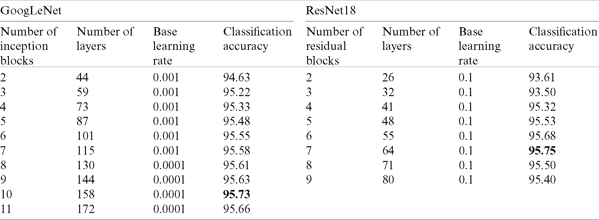
From Tab. 2, we notice the following:
• The accuracy of both models increases with the increase of the number of blocks until a certain threshold, 10 inception blocks for the GoogLeNet based model and 7 residual blocks for the ResNet18 based model. After this threshold, the accuracy starts decreasing in both models with the increase of the number of blocks.
• While the threshold of the residual network is lower than the number of the residual blocks in the original network (8 in ResNet18), the threshold in the inception network is higher than the number of inception blocks of the original network (9 in GoogLeNet).
Hence, the residual network with 6 or 7 blocks is selected as the solution because it has simpler architecture with slightly higher accuracy and lower training time, and surely it will have lower testing time. In the following subsections, fine-tuning will be performed to increase the accuracy of the residual solution.
4.4 Fine-Tuning of the Residual Solution
In this section, fine-tuning will be carried out by adding a drop-out layer with a proper drop-out rate (or probability) (DrOPr). Then the receptive field of the first CF will be varied to select the best size. Also, the hyper parameter, L2 Norm regularization factor (L2RF) will be tested to select the best value, and finally the rotation angle augmentation range will be experimented to determine the best range.
For instance, many other experiments have been performed to test the effects of other structural and parameter variations in the selected architecture, but most of them didn’t result in sensed improvements in the performance of the model such as changing the size of the filters inside the residual blocks to sizes other than
4.4.1 Testing the Effect of the Addition of a Drop-Out Layer Before the Fully Connected Layer
In this subsection, we test the effect of adding a drop-out layer before the fully connected one in four cases of the residual solution starting from the 5-block version until the 8-block version of the residual model and select the best DrOPr value (s) based on the attained accuracies in each case. We selected four cases to test because this modification affects the number of blocks to retain in our model in conjunction with the insertion of a drop-out layer with proper DrOPr. Since the 8-block version has the same layout as the original model of ResNet18 (with a 1-channel image input), hence we display only the layout of the 7-block residual network in Fig. 5 with the addition of a global variable named as Number of Filters (NF). The NF variable represents the number of CFs in the first residual block that is doubled every time down-sampling with a factor of 2 is performed in the subsequent blocks. The 6-block network is the resultant network after the removal of the seventh block and changing the average pooling to get the average of
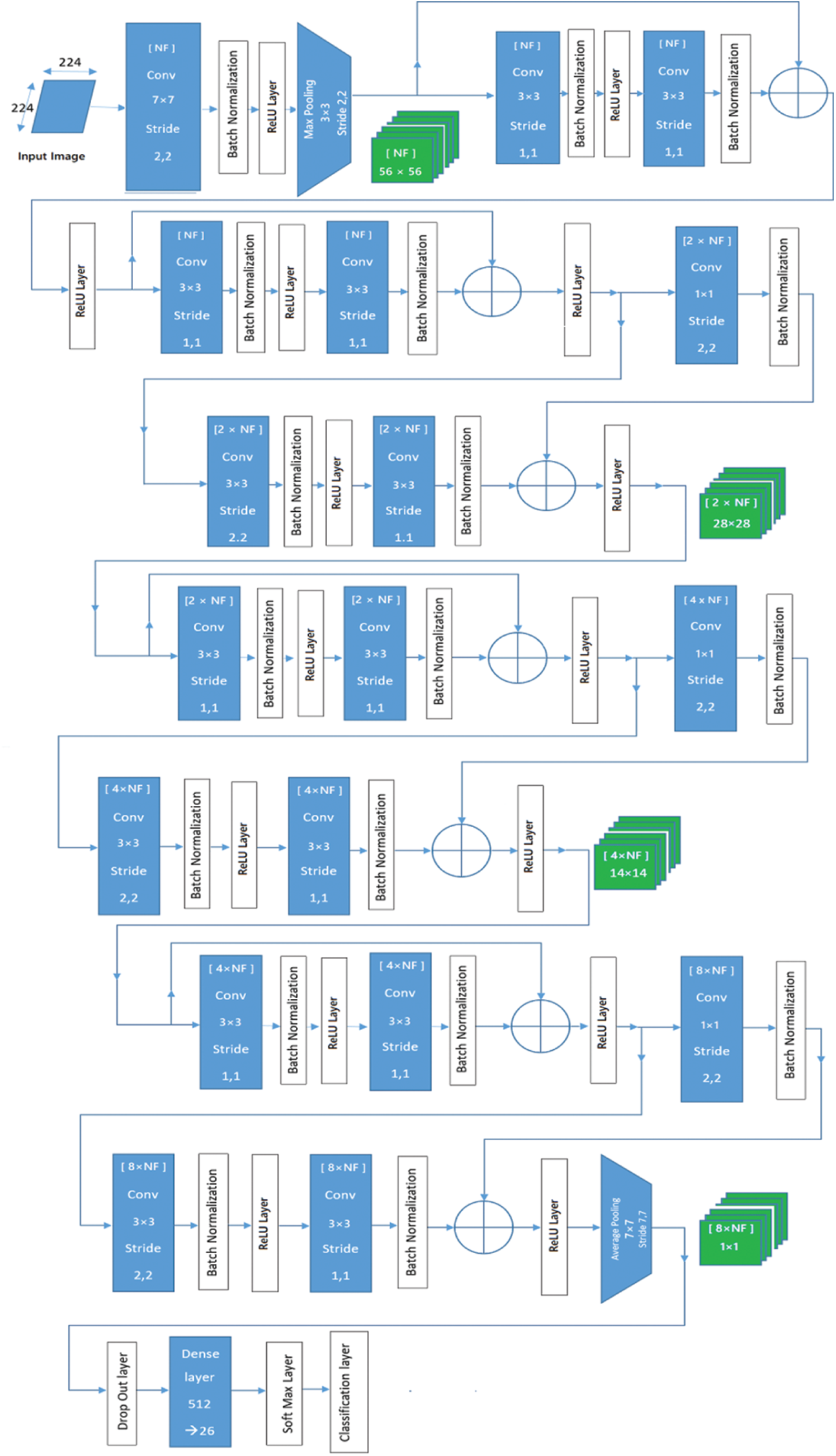
Figure 5: The 7-block residual CNN network, where the number of CFs is denoted by the number enclosed within brackets in the convolution unit and the resultant number of FMs is also denoted by the number enclosed within brackets in the multi-channel symbols that are not connected to the graph
Twenty-eight experiments have been performed by adding a drop-out layer before the fully connected layer in the 5-block until the 8-block versions and changing DrOPr from 0.2 to 0.8 to find the best layout with the best DrOPr value. Training using SGDM continues for 24 epochs, with a drop factor of 0.1 every 8 epochs. The results of the average accuracy in each case are shown in Tab. 3.
Table 3: The classification accuracy vs. the drop-out probability (DrOPr) in case of 5-block, 6-block, 7-block, and 8-block residual networks when applied to the EMNIST Letters dataset section
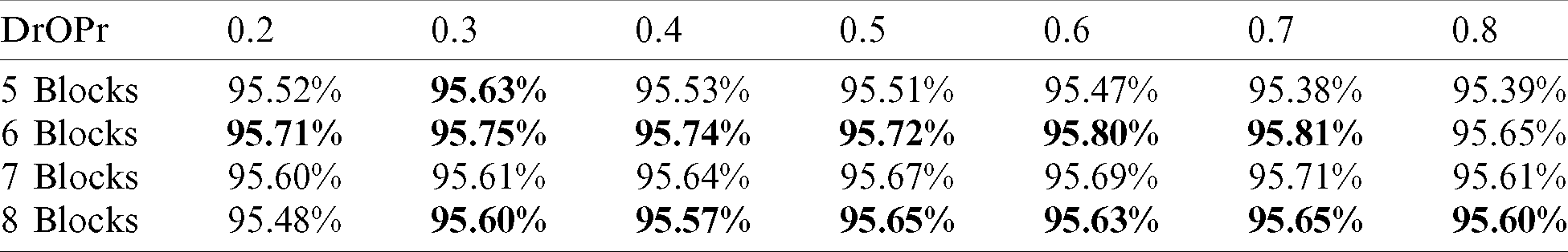
From Tab. 3, we notice that the drop-out layer enhances the 5-block and 6-block versions (bold values) while it does not enhance the 7-block version. The 8-block version is enhanced slightly, but still has a lower accuracy than intended. Moreover, we can conclude that adding a drop-out layer gives higher accuracy than adding an extra residual block at the end of the residual network (sure after reaching a certain threshold). We also deduce that the best drop-out probability is 0.7 for the 6-block case, which has an enhanced accuracy of 95.81%.
Hence, the 7th and 8th blocks will be removed, and we will present further modifications of the 6-block version in the following subsections.
4.4.2 Testing the Effect of the Size of the First CF
The first CF in ResNet18 has a
The first max-pooling filter is replaced by an average pooling filter to get more stable results because the max-pooling filter increases the character stroke thickness, while the average pooling filter smooths the edges of the character strokes without increasing their thickness. Tab. 4 shows the corresponding accuracy found for each filter size when using [
Table 4: The classification accuracy vs. the first CF size in case of the 6-block residual network
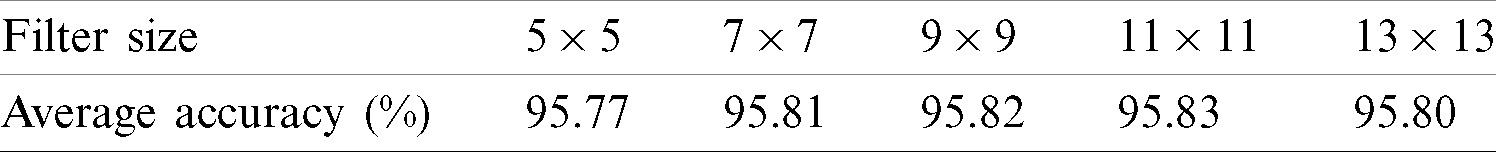
From this experiment, we can conclude that increasing the receptive field of the first filter to
Hence, we selected the two models with the
4.4.3 Testing the Effect of the L2 Norm Regularization Factor Value (L2RF)
The purpose of the L2 Norm regularization is to reduce overfitting by controlling change in the network (filters) weights during the optimization process through the regularization factor [26].
In this subsection, L2RF is changed from 0.0001 to 0.0009 and the resultant accuracy is recorded in each case for the
Tab. 5 lists the results of eighteen experiments done under the best conditions of the previous experiments (having a drop-out layer with probability 0.7, [
Table 5: The classification accuracy vs. the L2 regularization factor value
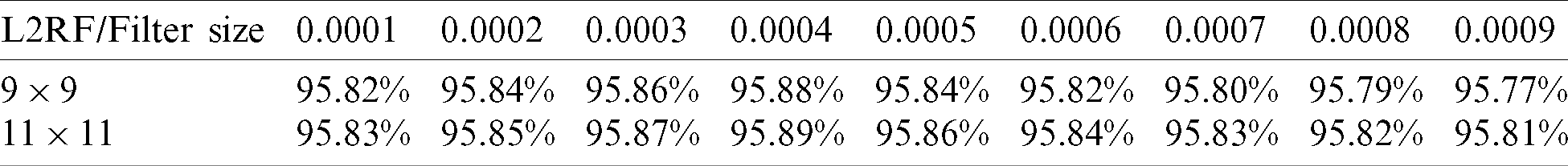
From Tab. 5, it can be concluded that the two values (0.0003 and 0.0004) of L2RF enhance the resulting average classification accuracy by about 0.05%, or in other words increase the number of correctly recognized characters by approximately 10 characters. Hence we select the value of 0.0004, which gave the highest average accuracy for the
4.4.4 Testing the Effects of Changing the Rotation Angle Augmentation Range
In this experiment we tested the
Table 6: The classification accuracy vs. the rotation angle augmentation range
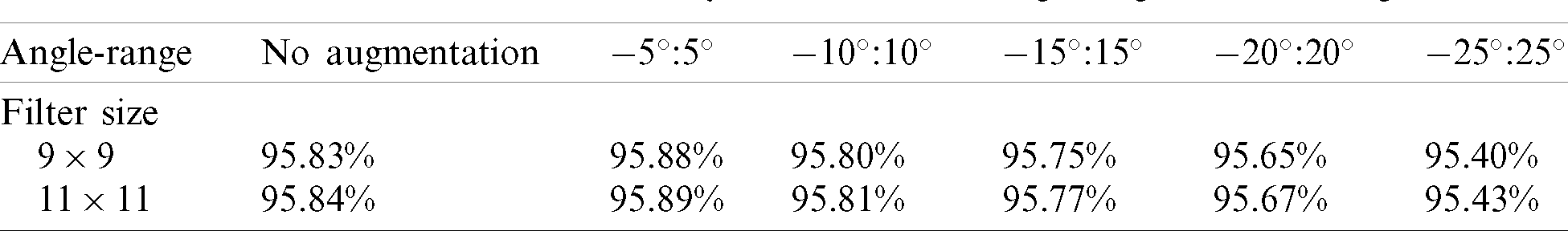
From Tab. 6, it appears that the best rotation angle augmentation range is [
4.4.5 Testing the Effect of Changing the Final Addition Layer into a Depth Concatenation Layer
Although changing the addition layer into a concatenation layer is a structural variation that should be done first with other structural variations, it has been delayed because it is a foreign variation where the modified model will no longer be a pure residual network. It is known that information is propagated through the residual network from block to block by keeping the original information and the mapped one in each level throughout the addition operation such that the output of the final block can be considered as the sum of all the outputs of the previous blocks (if we neglect the non-linear effects of the ReLU layers) as in (3). If we replace the final addition layer with a depth concatenation layer, we present the information of the penultimate residual block and the mapped information out of the final block in separate channels (FMs) instead of merging them through addition in the same channels (FMs). Although this type of information merging when implemented in the whole network proved superior in the previously developed DenseNet [27] when applied to the ImageNet, it did not show such superiority when tested without modifications on the EMNIST Letters dataset.
To illustrate the difference, we rewrite the recursive formula (3) in case of a Dense block of N modules as follows:
where the operator ‘
Although DenseNet is one of the important advanced architectures of the DCNN, we didn’t refer to it in the start of this research because its available ready-made models are considered heavyweight when compared with GoogLeNet and ResNet18.
A 1-channel version of DenseNet-BC-121 after being trained on the EMNIST Letters for 30 epochs with 0.1 drop factor every 6 epochs yielded an accuracy of 95.62% on the test set. It took about 111.7 hours of training compared to 4.15 hours for the ResNet18 and 10.04 hours for the GoogleNet that yielded accuracies of 95.50% and 95.63%, respectively as shown in Tab. 1.
This is because unlike the ImageNet, the images of the characters in the EMNIST dataset have single scale and mainly appear as a whole (not partially), and hence no need to give the representations in the earlier layers (or blocks) separate channels in the final layers (or blocks), which will increase the redundant information at the input of the final block.
Hence, we exchanged the addition layer with depth concatenation layer only in the final block and recorded the resulting accuracy after making the different types of parameter tuning, as done before.
Based on many experiments, we found that the best parameters are all the same as given in the previous subsections except the L2RF value, which is changed to 0.0005 to get the highest accuracy.
The resulting output of the final dense block, which is preceded by 5 residual blocks (Dense1Res5Out) can be represented by the following formula:
where
In the general case if there are R residual modules and D dense final modules we call this architecture DenseDResR. This is the reason that we referred to our final model defined in (5) by Dense1Res5.
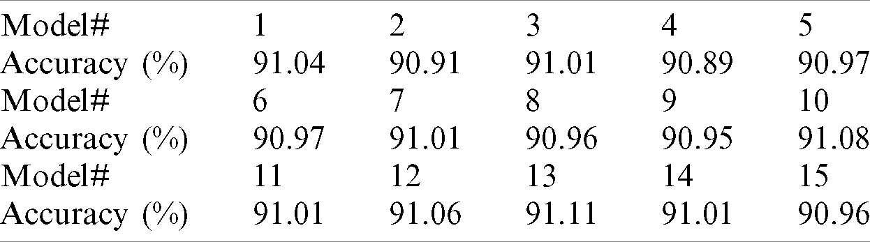
After repeating the training of the new network architecture fifteen times and recording the accuracies of the generated models on the Letters test set, we got the accuracy values listed in Tab. 7.
Table 7: The accuracy of the fifteen trained models when each is used to classify the letters test set
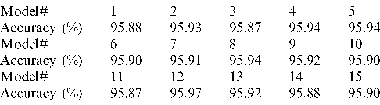
Hence, we conclude that the accuracy of the proposed model has a mean value of 95.91% with a standard deviation (STD) of 0.0003. For instance, we have replaced the last two blocks (
4.5 Aggregation of Different Instances of the Proposed Model
By selecting m models randomly out of the 15 models generated in the previous experiment we estimate the accuracy of the aggregated models based on the average of the class probabilities of the m models.
By performing 1000 random permutations for each value of m starting from 2 up to 9 and calculating the mean and standard deviation in each case, we got the results shown in Tab. 8 and plotted in Fig. 6.
Table 8: The mean and standard deviation of the classification accuracy of the Letters test set vs. the number of aggregated models (m)
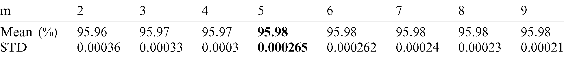
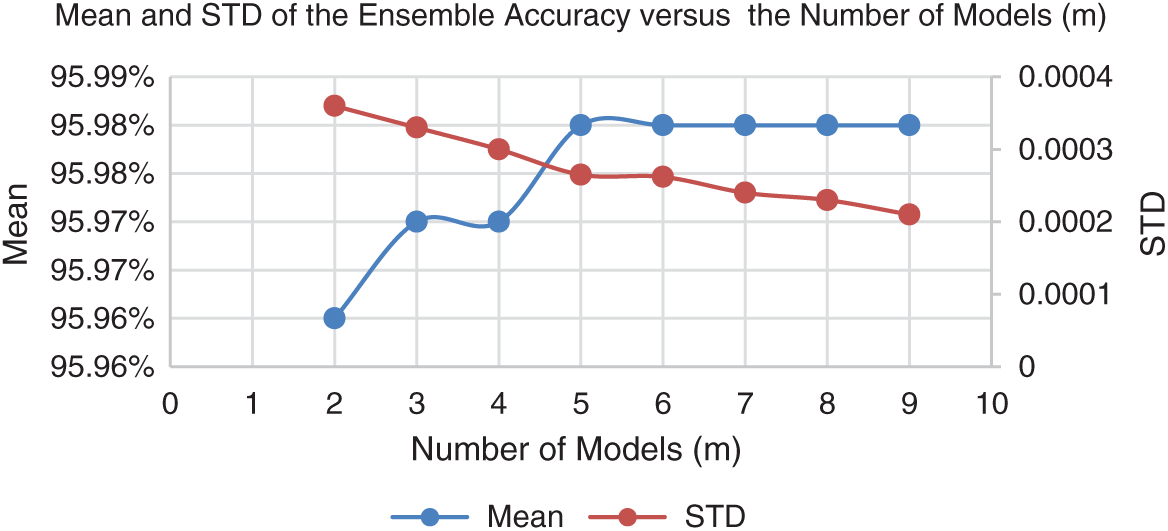
Figure 6: Mean and STD of the ensemble accuracy vs. the number of models (m)
Since our goal is to maximize the mean and minimize the STD of the classification accuracy without increasing the training and testing time too much, we will allow m to be increased as long as there are sensed improvements in the mean or in the STD to some extent.
From Tab. 8 and Fig. 6, we observe that the mean reaches its maximum at m = 5 (95.98%) and remains constant after that, while the STD has a value of
In this section, the final experiments are performed on the Balanced dataset section, and the results of both dataset sections are summarized when using a single model or an ensemble under the best conditions of the proposed models (Res6BF11 and Dense1Res5), which have a drop-out probability of 0.7 and a regularization factor of 0.0004 for Res6BF11 and 0.0005 for Dense1Res5 and using [
Then, the same experiments are repeated on both dataset sections but with training on a reduced dataset having 200 samples per class instead of 4800 samples per class in the Letters dataset and 2400 samples per class in the Balanced dataset respectively.
5.1 Experiments on the Balanced Dataset Section
In this subsection, the proposed models are applied to the Balanced dataset section, but an extra experiment will be carried out to test the effect of doubling the number of CFs (
When we applied the Res6BF11 and Dense1Res5 models to the Balanced dataset section, we got an average accuracy of 90.75% and 90.82%, respectively but when we doubled the number of CFs (
Table 9: The accuracy of fifteen versions of Dense1Res5 (
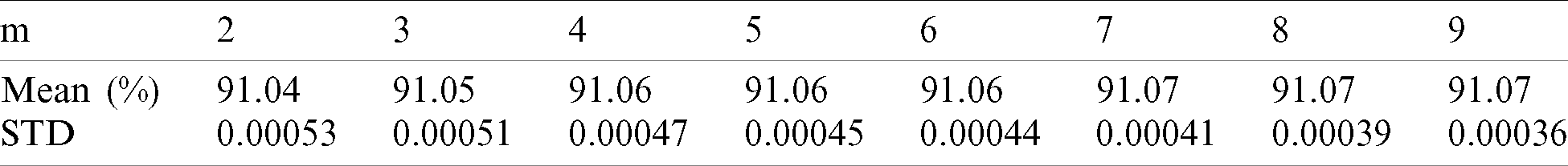
From Tab. 9, the mean is 91.00% and STD is
Tab. 10 gives the results of the aggregation of m models out of the fifteen versions. From Tab. 10, the mean when using 5 models is 91.06% and STD is
Table 10: The mean and standard deviation of the classification accuracy of the balanced test set vs. the number of aggregated models (m)
5.2 Testing the Proposed Models on the Reduced Training Dataset of the EMNIST Letters Section
We trained the Res6BF11 and Dense1Res5 models on the reduced training letters dataset section but with rotation angle augmentation range of [
For Res6BF11 and Dense1Res5 models with
Tab. 11 shows the resultant accuracies of fifteen experiments done with the Dense1Res5 model (
Table 11: The accuracy of fifteen versions of Dense1Res5 model (
5.3 Testing the Proposed Models on the Reduced Training Dataset of the EMNIST Balanced Section
We trained the Res6BF11 and Dense1Res5 models on the reduced training dataset section using a rotation angle augmentation range of [
Table 12: The accuracy of fifteen versions of Dense1Res5 model (
When we used an ensemble of 5 models of the fifteen Dense1Res5 versions, we got a mean accuracy of 88.83% (
6 Comparisons with State-of-the-Art Results
Tab. 13 summarizes the results for the full data set and the reduced one giving the accuracies of the proposed solutions (Res6BF11 and Dense1Res5 for
Table 13: Classification accuracy of the proposed models and the state-of-the-art systems for the full and reduced training sets of the Letters and Balanced dataset sections
Based on Tab. 13 and considering the results of the Letters dataset, we have increased the accuracy from the highest published value 95.58% to 95.98%, which is equivalent to decreasing the error rate by 9% using five Dense1Res5 (
Considering the Balanced dataset, we have increased the accuracy from the highest published value 90.59% to 91.06% which is equivalent to decreasing the error rate by 5% using five Dense1Res5 (
Considering the reduced training set of the Letters and Balanced datasets, we have increased the accuracies by 1.15% and 1.01%, respectively, over the TextCaps model published results, which is equivalent to decreasing the error rate by 15.95% and 8.29%, respectively.
Based on the testing done by [9] using the basic architecture of ResNet [18] on the Letters dataset, we have increased the accuracy of the basic ResNet architecture from 94.44% to 95.91% using a single instance of the Dense1Res5 (
Although the enhancements due to the replacement of the addition layer with the depth concatenation layer appear to be very small in the results of the full Letters dataset test (0.01% (
When we compare our work with the base model as done in most of the mentioned researches, we conclude that the accuracy has been increased by 10.83% and 13.04% for the Letters and Balanced datasets, respectively.
To allow reproducibility of the results and prevent any missing information in the proposed model, the MATLAB code that defines the layer graph of the Dense1Res5 model is listed in Appendix A.
In this research, the recognition accuracy of the EMNIST dataset using deep residual CNN has been improved by the following solution dimensions:
• Data dimension: the dataset images have been adapted with the residual CNN using the proper zero paddings and scaling and then proper rotation and shear angle augmentation have been performed to increase the trained model’s generalization.
• Structure dimension: the architecture of the residual solution has been enhanced by the selection of the optimum number of residual blocks, the optimum size of the receptive field of the first CF, the replacement of the first max-pooling layer with an average pooling layer, and the addition of the drop-out layer before the fully connected layer. A novel enhancement of the architecture has been achieved by replacing the final addition layer with a depth concatenation layer. Furthermore, doubling up the number of filters in all convolutional layers has brought enhancements in the subsequent accuracy, particularly in the Balanced dataset.
• Training hyperparameter dimension: the hyperparameters (learning rate, L2 regularization factor, mini-batch size, and the number of epochs in the training process) have been optimized for each proposed model in the four dataset cases (full Letters and Balanced datasets and their reduced versions).
• Aggregation of several models: by averaging the class probabilities of 5 versions of each proposed model the overall accuracy has been improved.
The improvements done to the residual solution starting with image scaling and data augmentation and ending with the hyperparameter optimization, resulted in a 26.43% improvement in the error rate in the classification of the EMNIST letters test set, relative to the basic residual architecture.
After using an ensemble of 5 versions of each proposed model, the improvements in the error rates relative to the stat-of-the-arts error rates become approximately 9%/5% for the full Letters/Balanced datasets and 16%/8% for the reduced training sets of the Letters/Balanced datasets, respectively.
The mentioned improvements in the residual DCNN model allowed the modified model to outperform the state-of-the-art models such as the TextCaps model in the classification of the handwritten characters when using either a huge training dataset or a reduced one.
On the basis of the experiments conducted in this work, we have also reached the following general conclusions for ResNet18 or similar architectures when being utilized in handwritten character image classification tasks:
• There is an optimal resolution of the input layer, in which the original image takes an optimal proportion that gives the maximum accuracy for a certain network architecture.
• Using rotation angle augmentation range of [
• There is an optimal number (Nopt) of residual blocks after which the accuracy does not improve or slightly decreases.
• Using (Nopt-1) blocks with a drop-out layer results in higher accuracy than using (Nopt) blocks even if a drop-out layer is used.
• Finalizing the residual net with a depth concatenated block generates a more accurate model than using a pure residual network when dealing with handwritten characters that have an approximately single scale and appear mostly in full shapes.
With regards to the architectures of DCNN, we have come up with a novel architecture which combined the residual network with the dense network in a sequential manner and offered a recursive definition for the original architectures and the new one, termed DenseDResR that could be evaluated in the future works with varying values of D and R on other dataset variants. We also gave an explanation why depth concatenation was beneficial in the final block only in the case of the EMNIST dataset based on the existence of full shapes of the characters in almost one scale in all the data set images. Other problems which give a decision of the presence of a class based on different scales of its shape or the partial existence of its shape such as ImageNet are expected to have a large D and small R where the lower abstractions of a shape (part of a circle for example) affect the final decision of the network and hence take a proportion in the final feature representation or abstraction. We think that using a large D irrelevant to the classification problem under consideration will introduce redundancy in the final and possibly in the intermediate layers of a network that will increase the memory requirements and the training time without having significant improvements in the resultant accuracy.
Acknowledgement: The authors acknowledge Prof. Abdullah Basuhail who supervises the Thesis of Mr. Hadi and did the proofreading of this paper.
Funding Statement: The authors received no specific funding for this study.
Conflicts of Interest: The authors declare that they have no conflicts of interest to report regarding the present study.
1. G. Cohen, S. Afshar, J. Tapson and A. Van Schaik. (2017). “EMNIST: Extending MNIST to handwritten letters,” in Proc. IJCNN 2017, Anchorage, AK, USA, pp. 2921–2926. [Google Scholar]
2. Y. LeCun, C. Cortes and C. BURGES. (2012). “The MNIST database of handwritten digits,” . [Online]. Available: http://yann.lecun.com/exdb/mnist/. [Google Scholar]
3. A. Baldominos, Y. Saez and P. Isasi. (2019). “A survey of handwritten character recognition with MNIST and EMNIST,” Applied Sciences, vol. 9, no. 15, pp. 3169. [Google Scholar]
4. A. van Schaik and J. Tapson. (2015). “Online and adaptive pseudoinverse solutions for ELM weights,” Neurocomputing, vol. 149, pp. 233–238. [Google Scholar]
5. Y. Peng and H. Yin. (2017). “Markov random field based convolutional neural networks for image classification,” Proc. IDEAL, vol. 10585, pp. 387–396. [Google Scholar]
6. P. Ghadekar, S. Ingole and D. Sonone. (2018). “Handwritten digit and letter recognition using hybrid DWT-DCT with KNN and SVM classifier,” in Proc. ICCUBEA, Pune, India, pp. 1–6. [Google Scholar]
7. R. Wiyatno and J. Orchard. (2018). “Style memory: Making a classifier network generative,” in Proc. (ICCI*CCBerkeley, CA, USA, pp. 16–21. [Google Scholar]
8. E. Dufourq and B. A. Bassett. (2017). “Eden: Evolutionary deep networks for efficient machine learning,” in Proc. (PRASA-RobMechBloemfontein, South Africa, pp. 110–115. [Google Scholar]
9. B. Ma, X. Li, Y. Xia and Y. Zhang. (2020). “Autonomous deep learning: A genetic DCNN designer for image classification,” Neurocomputing, vol. 379, pp. 152–161. [Google Scholar]
10. A. Baldominos, Y. Saez and P. Isasi. (2019). “Hybridizing evolutionary computation and deep neural networks: An approach to handwriting recognition using committees and transfer learning,” Complexity, vol. 2019, pp. 1–16. [Google Scholar]
11. P. Cavalin and L. Oliveira. (2018). “Confusion matrix-based building of hierarchical classification,” in Proc. Iberoamerican Congress on Pattern Recognition, CIARP, Madrid, Spain, pp. 271–278. [Google Scholar]
12. V. Jayasundara, S. Jayasekara, H. Jayasekara, J. Rajasegaran, S. Seneviratne et al. (2019). , “Textcaps: Handwritten character recognition with very small datasets,” in Proc. WACV, Waikoloa Village, HI, USA, pp. 254–262. [Google Scholar]
13. S. Sabour, N. Frosst and G. E. Hinton. (2017). “Dynamic routing between capsules,” in Advances in Neural Information Processing Systems, NIPS 2017. Long Beach, CA, USA: NEURAL INFORMATION PROCESSING SYSTEMS (NIPSpp. 3856–3866. [Google Scholar]
14. K. S. Younis. (2017). “Arabic handwritten character recognition based on deep convolutional neural networks,” Jordanian Journal of Computers and Information Technology, vol. 3, no. 3, pp. 186–200. [Google Scholar]
15. A. Shawon, M. J. U. Rahman, F. Mahmud and M. A. Zaman. (2018). “Bangla handwritten digit recognition using deep CNN for large and unbiased dataset,” in Proc. ICBSLP, Sylhet, Bangladesh, pp. 1–6. [Google Scholar]
16. A. Khan, A. Sohail, U. Zahoora and A. S. Qureshi. (2020). “A survey of the recent architectures of deep convolutional neural networks,” Artificial Intelligence Review, vol. 53, no. 8, pp. 5455–5516. [Google Scholar]
17. C. Szegedy, W. Liu, Y. Jia, P. Sermanet, S. Reed et al. (2015). , “Going deeper with convolutions,” in Proc. CVPR, Boston, MA, USA, pp. 1–9. [Google Scholar]
18. K. He, X. Zhang, S. Ren and J. Sun. (2016). “Deep residual learning for image recognition,” in Proc. CVPR, Las Vegas, NV, USA, pp. 770–778. [Google Scholar]
19. S. Ioffe and C. Szegedy. (2015). “Batch normalization: Accelerating deep network training by reducing internal covariate shift,” arXiv preprint, arXiv:1502.03167. [Google Scholar]
20. N. Srivastava, G. Hinton, A. Krizhevsky, I. Sutskever and R. Salakhutdinov. (2014). “Dropout: A simple way to prevent neural networks from overfitting,” Journal of Machine Learning Research, vol. 15, no. 1, pp. 1929–1958. [Google Scholar]
21. X. Lin, Y. L. Ma, L. Z. Ma and R. L. Zhang. (2014). “A survey for image resizing,” Journal of Zhejiang University SCIENCE C, vol. 15, no. 9, pp. 697–716. [Google Scholar]
22. A. Poznanski and L. Wolf. (2016). “CNN-N-Gram for handwriting word recognition,” in Proc. CVPR, Las Vegas, NV, USA, pp. 2305–2314. [Google Scholar]
23. Y. Yan, T. Yang, Z. Li, Q. Lin and Y. Yang. (2018). “A unified analysis of stochastic momentum methods for deep learning,” arXiv preprint, arXiv:1808.07576. [Google Scholar]
24. Z. L. Ke, H. Y. Cheng and C. L. Yang. (2018). “LIRS: Enabling efficient machine learning on NVM-based storage via a lightweight implementation of random shuffling,” arXiv preprint, arXiv:1810.04509. [Google Scholar]
25. D. P. Kingma and J. Ba. (2014). “Adam: A method for stochastic optimization,” arXiv preprint, arXiv:1412.6980. [Google Scholar]
26. P. Murugan and S. Durairaj. (2017). “Regularization and optimization strategies in deep convolutional neural network,” arXiv preprint, arXiv:1712.04711. [Google Scholar]
27. G. Huang, Z. Liu, L. Van Der Maaten and K. Q. Weinberger. (2017). “Densely connected convolutional networks,” in Proc. CVPR, Honolulu, HI, USA, pp. 4700–4708. [Google Scholar]
Appendix A. Dense1Res5 Lgraph Creation Code
% Script for creating the layers for a deep-learning network with: Number of layers: 57, Number of connections: 62
% Running this script will create the layers in the workspace variable lgraph.
% Create the layer graph variable to contain the network’s layers.
lgraph = layerGraph( );
% Add the Layer Branches, Add the branches of the network to the layer graph, Each branch is a linear array of layers.
tempLayers = [
imageInputLayer([224,224,1],“Name”, “data”, “Normalization”, “none”)
batchNormalizationLayer(“Name”, “bn_conv1_1_2”)
convolution2dLayer([11,11], NF, “Name”, “conv1_1”, “BiasLearnRateFactor”, 0, “Padding”, [5 5 5 5], “Stride”, [2 2])
batchNormalizationLayer(“Name”, “bn_conv1_1_1”)
reluLayer(“Name”, “conv1_relu”)
averagePooling2dLayer([3,3], “Name”, “avgpool2d”, “Padding”, [1 1 1 1], “Stride”, [2 2])];
lgraph = addLayers(lgraph,tempLayers);
tempLayers = [
convolution2dLayer([3,3], NF, “Name”, “res2a_branch2a”, “BiasLearnRateFactor”, 0, “Padding”, [1 1 1 1])
batchNormalizationLayer(“Name”, “bn2a_branch2a”)
reluLayer(“Name”, “res2a_branch2a_relu”)
convolution2dLayer([3,3], NF, “Name”, “res2a_branch2b”, “BiasLearnRateFactor”, 0, “Padding”, [1 1 1 1])
batchNormalizationLayer(“Name”, “bn2a_branch2b”)];
lgraph = addLayers(lgraph, tempLayers);
tempLayers = [additionLayer(2, “Name”, “res2a”)
reluLayer(“Name”, “res2a_relu”)];
lgraph = addLayers(lgraph, tempLayers);
tempLayers = [
convolution2dLayer([3,3], NF, “Name”, “res2b_branch2a”, “BiasLearnRateFactor”, 0, “Padding”, [1 1 1 1])
batchNormalizationLayer(“Name”, “bn2b_branch2a”)
reluLayer(“Name”, “res2b_branch2a_relu”)
convolution2dLayer([3,3], NF, “Name”, “res2b_branch2b”, “BiasLearnRateFactor”, 0, “Padding”, [1 1 1 1])
batchNormalizationLayer(“Name”, “bn2b_branch2b”)];
lgraph = addLayers(lgraph, tempLayers);
tempLayers = [additionLayer(2, “Name”, “res2b”)
reluLayer(“Name”, “res2b_relu”)];
lgraph = addLayers(lgraph, tempLayers);
tempLayers = [
convolution2dLayer([1,1], 2 * NF, “Name”, “res3a_branch1”, “BiasLearnRateFactor”, 0, “Stride”, [2 2])
batchNormalizationLayer(“Name”, “bn3a_branch1”)];
lgraph = addLayers(lgraph, tempLayers);
tempLayers = [
convolution2dLayer([3,3], 2 * NF, “Name”, “res3a_branch2a”, “BiasLearnRateFactor”, 0, “Padding”, [1 1 1 1], “Stride”, [2 2])
batchNormalizationLayer(“Name”, “bn3a_branch2a”); reluLayer(“Name”, “res3a_branch2a_relu”)
convolution2dLayer([3,3],2 * NF, “Name”, “res3a_branch2b”, “BiasLearnRateFactor”, 0, “Padding”, [1 1 1 1])
batchNormalizationLayer(“Name”, “bn3a_branch2b”)];
lgraph = addLayers(lgraph, tempLayers);
tempLayers = [additionLayer(2, “Name”, “res3a”)
reluLayer(“Name”, “res3a_relu”)];
lgraph = addLayers(lgraph, tempLayers);
tempLayers = [
convolution2dLayer([3,3], 2 * NF, “Name”, “res3b_branch2a”, “BiasLearnRateFactor”, 0, “Padding”, [1 1 1 1])
batchNormalizationLayer(“Name”, “bn3b_branch2a”)
reluLayer(“Name”, “res3b_branch2a_relu”)
convolution2dLayer([3,3], 2 * NF, “Name”, “res3b_branch2b”, “BiasLearnRateFactor”, 0, “Padding”, [1 1 1 1])
batchNormalizationLayer(“Name”, “bn3b_branch2b”)];
lgraph = addLayers(lgraph, tempLayers);
tempLayers = [additionLayer(2, “Name”, “res3b”)
reluLayer(“Name”, “res3b_relu”)];
lgraph = addLayers(lgraph, tempLayers);
tempLayers = [
convolution2dLayer([1,1], 4 * NF, “Name”, “res4a_branch1”, “BiasLearnRateFactor”, 0, “Stride”, [2 2])
batchNormalizationLayer(“Name”, “bn4a_branch1”)];
lgraph = addLayers(lgraph, tempLayers);
tempLayers =
convolution2dLayer([3,3], 4 * NF, “Name”, “res4a_branch2a”, “BiasLearnRateFactor”, 0, “Padding”, [1 1 1 1], “Stride”, [2 2])
batchNormalizationLayer(“Name”, “bn4a_branch2a”)
reluLayer(“Name”, “res4a_branch2a_relu”)
convolution2dLayer([3,3], 4 * NF, “Name”, “res4a_branch2b”, “BiasLearnRateFactor”, 0, “Padding”, [1 1 1 1])
batchNormalizationLayer(“Name”, “bn4a_branch2b”)];
lgraph = addLayers(lgraph, tempLayers);
tempLayers = [additionLayer(2, “Name”, “res4a”)
reluLayer(“Name”, “res4a_relu”)];
lgraph = addLayers(lgraph, tempLayers);
tempLayers = [
convolution2dLayer([3,3], 4 * NF, “Name”, “res4b_branch2a”, “BiasLearnRateFactor”, 0, “Padding”, [1 1 1 1])
batchNormalizationLayer(“Name”, “bn4b_branch2a”)
reluLayer(“Name”, “res4b_branch2a_relu”)
convolution2dLayer([3,3], 4 * NF, “Name”, “res4b_branch2b”, “BiasLearnRateFactor”, 0, “Padding”, [1 1 1 1])
batchNormalizationLayer(“Name”, “bn4b_branch2b”)];
lgraph = addLayers(lgraph, tempLayers);
tempLayers = [ depthConcatenationLayer(2, “Name”, “depthcat”)
reluLayer(“Name”, “res5a_relu”)
averagePooling2dLayer([14,14], “Name”, “avgpool2d_2”, “Stride”, [14 14])
dropoutLayer(0.7, “Name”, “dropout”)
fullyConnectedLayer(26, “Name”, “fc”, “BiasLearnRateFactor”, 2, “WeightLearnRateFactor”, 2)
softmaxLayer(“Name”, “prob”); classificationLayer(“Name”, “classoutput”)];
lgraph = addLayers(lgraph, tempLayers);
lgraph = connectLayers(lgraph, “avgpool2d”, “res2a_branch2a”);
lgraph = connectLayers(lgraph, “avgpool2d”, “res2a/in2”);
lgraph = connectLayers(lgraph, “bn2a_branch2b”, “res2a/in1”);
lgraph = connectLayers(lgraph, “res2a_relu”, “res2b_branch2a”);
lgraph = connectLayers(lgraph, “res2a_relu”, “res2b/in2”);
lgraph = connectLayers(lgraph, “bn2b_branch2b”, “res2b/in1”);
lgraph = connectLayers(lgraph, “res2b_relu”, “res3a_branch1”);
lgraph = connectLayers(lgraph, “res2b_relu”, “res3a_branch2a”);
lgraph = connectLayers(lgraph, “bn3a_branch1”, “res3a/in2”);
lgraph = connectLayers(lgraph, “bn3a_branch2b”, “res3a/in1”);
lgraph = connectLayers(lgraph, “res3a_relu”, “res3b_branch2a”);
lgraph = connectLayers(lgraph, “res3a_relu”, “res3b/in2”);
lgraph = connectLayers(lgraph, “bn3b_branch2b”, “res3b/in1”);
lgraph = connectLayers(lgraph, “res3b_relu”, “res4a_branch1”);
lgraph = connectLayers(lgraph, “res3b_relu”, “res4a_branch2a”);
lgraph = connectLayers(lgraph, “bn4a_branch1”, “res4a/in2”);
lgraph = connectLayers(lgraph, “bn4a_branch2b”, “res4a/in1”);
lgraph = connectLayers(lgraph, “res4a_relu”, “res4b_branch2a”);
lgraph = connectLayers(lgraph, “res4a_relu”, “depthcat/in2”);
lgraph = connectLayers(lgraph, “bn4b_branch2b”, “depthcat/in1”);
% Clean Up Helper Variable
clear tempLayers;
 | This work is licensed under a Creative Commons Attribution 4.0 International License, which permits unrestricted use, distribution, and reproduction in any medium, provided the original work is properly cited. |