Computers, Materials & Continua DOI:10.32604/cmc.2021.015710
Article

Numerical Solutions for Heat Transfer of An Unsteady Cavity with Viscous Heating

H. F. Wong1,2, Muhammad Sohail3, Z. Siri1 and N. F. M. Noor1,*

1Institute of Mathematical Sciences, Faculty of Science, University of Malaya, 50603 Kuala Lumpur, Malaysia
2Unit of Engineering Design and Product Development, Technology and Engineering Division, Malaysian Rubber Board, 47000 Sungai Buloh, Malaysia
3Department of Applied Mathematics & Statistics, Institute of Space Technology, 44000 Islamabad, Pakistan
*Corresponding Author: N. F. M. Noor. Email: drfadiya@um.edu.my
Received: 03 December 2020; Accepted: 15 January 2021

Abstract: The mechanism of viscous heating of a Newtonian fluid filled inside a cavity under the effect of an external applied force on the top lid is evaluated numerically in this exploration. The investigation is carried out by assuming a two-dimensional laminar in-compressible fluid flow subject to Neumann boundary conditions throughout the numerical iterations in a transient analysis. All the walls of the square cavity are perfectly insulated and the top moving lid produces a constant finite heat flux even though the fluid flow attains the steady-state condition. The objective is to examine the effects of viscous heating in the fully insulated lid-driven cavity under no-slip and free-slip Neumann boundary conditions coupled with variations in Reynolds and Prandtl numbers. The partial differential equations of time-dependent vorticity-stream function and thermal energy are discretized and solved using a self-developed finite difference code in MATLAB® environment. Time dependence of fluid thermodynamics is envisaged through contour and image plots. A commercial simulation software, Ansys Fluent® utilizing a finite element code is employed to verify the finite difference results produced. Although the effect of viscous heating is very minimal, Neumann no-slip and free-slip boundary conditions are able to trap the heat inside the fully insulated cavity as the heat flux is constantly supplied at the top lid. A lower Reynolds number and a greater Prandtl number with free-slip effects reduce temperature distribution in the cavity with a faster velocity than in the no-slip condition as the free-slip behaves as a lubricant.

Keywords: Lid-driven; viscous heating; vorticity-stream function; finite difference method; finite element method

Nomenclature

1  Introduction

Viscous heating is generated by a fluid’s viscous friction when the fluid is sheared by an external motion, provided the fluid is not inviscid and sluggish [1]. Viscous heating process is important in creating energy sources while Neumann boundary condition (BC) is important in renewable energy applications such as in energy saving or to increase energy efficiency in buildings. Viscous heating is studied in a slipped flow region using a free-slip boundary condition by Mohamed [2]. His study shows a momentous effect on the heat transfer and fluid flow peculiarity in microchannel studies even though the fluid has tenuous viscous flow and possesses a tiny value of hydraulic diameter. Koo et al. [3] discovered that viscous dissipation is effectively influenced by Reynolds number and geometrical aspect ratio. The viscous dissipation effect on free-slip BC is also discussed by Rij et al. [4,5] in a 3D micro-channel gas flow where it is dependent on the amount of rarefaction and other factors.

Another important study of viscous dissipation merged with Joule heating, carried out by Kumar et al. [6], shows an upward trend of temperature distribution in a non-Newtonian fluid flow. The heat transfer process of a Newtonian fluid which takes into account the viscous dissipation in a fully-developed region was performed using an explicit numerical method [7]. The variation of the heat transfer process presented an unusual degree in the fully-developed region, both hydro-dynamically and thermally, due to the thermal energy balance between the heated walls is combined with adiabatic walls and the viscous heating [8–10]. Other applications of combined Neumann BC and constant wall temperature can be discovered in magnetized nanofluids in a porous cylinder [11], buoyancy effects [12], open trapezoidal cavity [13] and in variation of heat source lengths [14]. The catastrophe such as the source of heat in storm or hurricane is derived from the viscous dissipation near the surface [15] and it can be estimated via the turbulent kinetic energy [16] where the heat viscous dissipation is a cubic function of the wind speed.

In some cases, such as in magneto-hydrodynamic (MHD) and mixed convection studies [17,18], the electrically conducting fluid motion is retarded by the magnetic field [19], hence it produces an insignificant viscous heating as compared with the amount of heat generated by a buoyancy force. Generalized differential quadrature method was utilized to study the MHD non-Newtonian nanofluid flow and the impacts of various physical properties [20]. Other numerical methods such as Gear–Chebyshev–Gauss–Lobatto collocation method [21] and the fourth-fifth-order Runge–Kutta–Fehlberg method [22] were used to solve an MHD nanofluid flow with a thermal radiation and an applied magnetic field respectively. The study of MHD flow was also conducted in a fluid thermal analysis where three modes of convection specifically referred as free, forced and Marangoni convections are considered [23]. Besides, Zhou et al. [24] examined Boussinesq approximation [25] in the thermal energy equation when a Newtonian fluid is subject to a mixed convection process with different heat sources in a lid-driven cavity. Rahman et al. [26] revealed that the velocity and temperature profiles of a lid-driven flow with a semi-circular heated wall are independent of the viscous heating when they are subject to magnetic field and Joule heating. Anderson [27] derived the thermal energy equation for a highly viscous flow which includes the viscous terms used to estimate the meteorite surface temperature. Newtonian homogenous and heterogenous nanofluids [28–31] can also be considered in the future studies as the occupying fluids in the cavity flows with viscous heating and slip effects.

The cited literatures [17–27] obviously show that viscous heating is important in fluid dynamics and thermal analyses where the viscous heating is comparable with other effects. The intention of this work is to utilize the lid-driven cavity model combined with Neumann BCs [32]. To make our analysis easier, the moving top lid is not taken into account in the heat transfer analysis thus it will be presumed as an insulator. In order to facilitate the calculations, all the governing equations employed in our paper are given in terms of the vorticity-stream function [33] and thermal energy equation [25]. Then we use an explicit finite difference method (FDM) to discretize all the governing equations and conduct the fluid flow and heat transfer analyses from an unsteady-state until the steady-state flow is achieved. Those results are then compared with the solutions of finite element method (FEM) using Ansys Fluent®. We also impose free-slip BC in the cavity model to investigate how the viscous heating process influences the temperature distribution inside the whole cavity.

2  Mathematical Model

The schematic drawing of a two-dimensional lid-driven cavity model within the Cartesian coordinate system is shown in Fig. 1. In this case, the external velocity, Uwall is imposed on the top lid, u and v are the velocity vectors in x and y directions, ρ and μ are fluid density and dynamic viscosity, ∂u∂y|x=0, ∂u∂y|x=L and ∂v∂x|y=0 are the velocity gradients along the fixed wall in x- and y-directions, H and L are height and length of the cavity. Subsequently, k and c are thermal conductivity and specific heat of the fluid, ∂T∂x|x=0, ∂T∂x|x=L and ∂T∂y|y=0are the temperature gradients along the fixed wall in x- and y-directions. The fluid flow process is presumed as two-dimensional, in-compressible, laminar and the Newtonian fluid properties are not in the function of temperature or they behave as constants. Then the buoyancy force is excluded from the heat transfer analysis as the heat flux (due to viscous heating) is generated from the moving top lid. Therefore, no convection occurs from the bottom fixed lid to the top moving lid while Boussinesq approximation [25] is not included in the thermal energy equation. The top moving lid is presumed fully insulated.

Figure 1: Schematic drawing of a 2D cavity flow with Neumann BC

The continuity and governing equations for the two-dimensional in-compressible viscous unsteady Newtonian fluid flow in x- and y-directions are given by [34]

∂u∂x+∂v∂y=0, (1)

ρ[∂u∂t+u∂u∂x+v∂u∂y]=-∂p∂x+ρgx+μ(∂2u∂x2+∂2u∂y2), (2)

ρ[∂v∂t+u∂v∂x+v∂v∂y]=-∂p∂y+ρgy+μ(∂2v∂x2+∂2v∂y2),

where t is time and gx = gy = g is gravity acceleration. The curl [35] of Eqs. (2) and (3) is known as vorticity-stream function scheme or vorticity transport equation and it is given by [33] as

∂ζ∂t-∂ψ∂x∂ζ∂y+∂ψ∂y∂ζ∂x=μρ(∂2ζ∂x2+∂2ζ∂y2),(3)

where stream function, ψ is given by Eqs. (5) and (6) while vorticity, ζ is given by Eq. (7),

u=∂ψ∂y, (5)

v=-∂ψ∂x, (6)

ζ=∂v∂x-∂u∂y.

The vorticity, ζ at the moving top lid can be obtained via Taylor series expansion [36] and it is given by:

top moving lid BC:ζtop=-2(ψi,j=2-ψi,j=1)Δy2+2UwallΔy.(7)

The vorticity, ζ at the left, right and bottom walls for the free-slip BC are given by:

bottomBC:ζbottom=-(ψi,j=ny-1-ψi,j=ny)lsΔy+Δy22, (9)

leftBC:ζleft=-(ψi=2,j-ψi=1,j)lsΔx+Δx22 (10)

rightBC:ζright=-(ψi=nx-1,j-ψi=nx,j)lsΔx+Δx22

where Δx=Δy=h is the step size, j is the row, i is the column, n is the number of nodes and ls is a slip length. If the slip length, ls is equal to zero, Eq. (9) till Eq. (11) can be used for vorticity, ζ at the left, right and bottom walls for the no-slip BC respectively.

Two-dimensional unsteady thermal energy equation [25] which includes the effect of viscous dissipation is given by

∂T∂t+u∂T∂x+v∂T∂y=kρc(∂2T∂x2+∂2T∂y2)+μρc[(∂u∂y+∂v∂x)2+2(∂u∂x)2+2(∂v∂y)2],(11)

where T is a temperature. Substituting Eqs. (5) and (6) into Eq. (12) will result in

∂T∂t+∂ψ∂y∂T∂x-∂ψ∂x∂T∂y=kρc(∂2T∂x2+∂2T∂y2)+μρc[(∂2ψ∂y2-∂2ψ∂x2)2+4(∂2ψ∂x∂y)2].(13)

The temperature, T at each of the walls and at each of the corners can be obtained by introducing Neumann BC [32] in the unsteady-state condition where they are given by

top moving lid BC:Ti,j=1t+1=λ(2Ti,j+1t+Ti-1,jt+Ti+1,jt)+(1-4λ)Ti,j=1t, (14)

bottom BC:Ti,j=nyt+1=λ(2Ti,j-1t+Ti-1,jt+Ti+1,jt)+(1-4λ)Ti,j=nyt, (15)

leftBC:Ti=1,jt+1=λ(2Ti+1,jt+Ti,j+1t+Ti,j-1t)+(1-4λ)Ti=1,jt,

right BC:Ti=nx,jt+1=λ(2Ti-1,jt+Ti,j+1t+Ti,j-1t)+(1-4λ)Ti=nx,jt,

top left corner BC:Ti=1,j=1t+1=2λ(Ti+1,jt+Ti,j+1t)+(1-4λ)Ti=1,j=1t,

top right corner BC:Ti=nx,j=1t+1=2λ(Ti-1,jt+Ti,j+1t)+(1-4λ)Ti=nx,j=1t,

bottom left corner BC:Ti=1,j=nyt+1=2λ(Ti+1,jt+Ti,j-1t)+(1-4λ)Ti=1,j=nyt,

bottom right corner BC:Ti=nx,j=nyt+1=2λ(Ti-1,jt+Ti,j-1t)+(1-4λ)Ti=nx,j=nyt,

where λ=kΔtρch2 is Fourier number, Δt is a time step and t is the current time step.

3  Numerical Method

In this section, some matters related to numerical modelling for solution of the two-dimensional vorticity transport equation and thermal energy equation will be discussed. These issues are applications of the simplest numerical method, stability issue and iteration algorithm. Since Eq. (4) and Eq. (13) are nonlinear second-order partial differential equations, an explicit FDM is the simplest method among the feasible techniques for the numerical solution. However, it is conditionally stable [33]. Eqs. (4) and (13) can be transformed into equivalent finite difference equations (FDE) using forward and central finite-divided-difference formulas.

ζi,jt+1-ζi,jtΔt=-(ψi,j+1t-ψi,j-1t2h)(ζi+1,jt-ζi-1,jt2h)+(ψi+1,jt-ψi-1,jt2h)(ζi,j+1t-ζi,j-1t2h)+μρ(ζi+1,jt+ζi-1,jt+ζi,j+1t+ζi,j-1t-4ζi,jth2)(16)

Rearranging Eq. (22) yields

ζi,jt+1=-Δt[(ψi,j+1t-ψi,j-1t2h)(ζi+1,jt-ζi-1,jt2h)-(ψi+1,jt-ψi-1,jt2h)(ζi,j+1t-ζi,j-1t2h)-μρ(ζi+1,jt+ζi-1,jt+ζi,j+1t+ζi,j-1th2)]+(1-4μΔtρh2)ζi,jt.(23)

Similarly, the resultant FDE for the thermal energy equation is given by

Ti,jt+1-Ti,jtΔt=-(ψi,j+1t-ψi,j-1t2h)(Ti+1,jt-Ti-1,jt2h)+(ψi+1,jt-ψi-1,jt2h)(Ti,j+1t-Ti,j-1t2h)+μρc[(ψi,j+1t+ψi,j-1t-ψi+1,jt-ψi-1,jth2)2+4(ψi+1,j+1t+ψi-1,j-1t-ψi+1,j-1t-ψi-1,j+1t4h2)2]+kρc(Ti+1,jt+Ti-1,jt+Ti,j+1t+Ti,j-1t-4Ti,jth2).(24)

Rearranging Eq. (24) yields

Ti,jt+1=Δt[-(ψi,j+1t-ψi,j-1t2h)(Ti+1,jt-Ti-1,jt2h)+(ψi+1,jt-ψi-1,jt2h)(Ti,j+1t-Ti,j-1t2h)+μρc[(ψi,j+1t+ψi,j-1t-ψi+1,jt-ψi-1,jth2)2+(ψi+1,j+1t+ψi-1,j-1t-ψi+1,j-1t-ψi-1,j+1t2h2)2]+kρc(Ti+1,jt+Ti-1,jt+Ti,j+1t+Ti,j-1th2)]+(1-4kΔtρch2)Ti,jt.(25)

From Eq. (23), the criterion is determined by requiring that the coefficient associated with the node of interest at the previous time is greater than or equal to zero [25], such that

(1-4μΔtρh2)≥0orΔt≤ρh24μ(26)

and from Eq. (24),

(1-4kΔtρch2)≥0orΔt≤ρch24k.(27)

Eqs. (26) and (27) are the conditional stability criteria. However, the maximum allowable time step, Δt should be evaluated again so that it can fulfill Eqs. (26) and (27). Thus, the adopted maximum allowable time step, Δtmax is given by

Δtmax=min(ρh24μ,ρch24k),(28)

where min ( ) means the smallest element is taken inside the bracket. Eq. (28) is called Poisson equation [32]. Substituting Eqs. (5) and (6) into Eq. (7) yields

-ζ=∂2ψ∂x2+∂2ψ∂y2.(29)

Similarly, Eq. (29) can be discretized using the FDE as follows:

ψi,jn+1=14(ψi+1,jn+ψi-1,jn+ψi,j+1n+ψi,j-1n+h2ζi,jn),(30)

where n is the number of iterations. Eq. (29) can later be solved by using Gauss–Seidel method [35]. The time-marching method to solve the forward FDE of the vorticity transport equation and thermal energy equation are carried out in MATLAB® environment following the procedure below:

Step I: Initial values of stream function, ψ and vorticity, ζ are set to zero at the first time step, t = 0. Values of stream function, ψ at the top, bottom, left and right boundaries are set to zero along the iterative process from the 1st time step, t = 0 till the last time step, t = tend.

Step II: The interior nodes of the stream function, ψ are solved using Eq. (29) by Gauss–Seidel method or any other method until all these values converge. In this paper, the convergence criterion of 10−5 is chosen [37].

Step III: The values of vorticity at those four boundaries, ζtop, ζbottom, ζleft and ζright are calculated using Eqs. (8)–(11).

Step IV: The interior nodes of vorticity, ζ are updated using Eq. (23). The maximum allowable time step, Δtmax is ensured to be within the limit prescribed by Eq. (28).

Step V: An initial value of temperature throughout the lid-driven is given. Then Eq. (25) is coupled to the function, ψ with the value obtained from Eq. (30). Similarly, the maximum allowable time step, tmax is utilized in Step IV.

Step VI: The values of temperature at those four walls and four corners namely Ti,j=1t+1, Ti,j=nyt+1, Ti=1,jt+1, Ti=nx,jt+1, Ti=1,j=1t+1, Ti=nx,j=1t+1, Ti=1,j=nyt+1, Ti=nx,j=nyt+1 are calculated using Eq. (14) till Eq. (21).

Step VII: Steps II–VI are repeated until the steady-state condition of the flow is achieved or at any desired time step.

4  Results and Analysis

In this study, the aspect ratio, A = 1 (1m×1m) will be used throughout our paper. There are six case studies considered to characterize the flow field and temperature distribution in the two-dimensional lid-driven cavity flow with insulated walls in order to understand the effect of viscous heating in both no-slip and free-slip Neumann BCs. The six test cases with different fluid properties and laminar unsteady flow conditions are performed in an iterative procedure until the analysis period, t = 1.5 s is achieved (longer than the steady-state criterion of e = 10−5). The applied velocity is Uwall = 10 m/s (except Uwall = 5 m/s in the 3rd and 4th test cases). The fluid density, ρ is set to 15 kg/m3, dynamic viscosity, μ = 2 Pa.s, thermal conductivity, k = 10 W/mK, specific heat, c=10J/kg⋅K (except c=20J/kg⋅K in the 5th and 6th cases) and initial temperature, Ti of the whole fluid inside the cavity is set to 25∘C. The time step, Δt is set to 0.001 s and the entire computation is performed on uniform grids 40 × 40 (Δx=Δy=h). The Prandtl number, Pr is defined as

Pr=να=cμk,(31)

where ν is a kinematic viscosity and α is a thermal diffusivity defined by

α=kρc.(32)

The Reynolds number, ReL can be reckoned via Eq. (33) [38] as

ReL=UwallρLμ,(33)

where L is height of the cavity. Then, free-slip BC with slip length value, ls = 1 m is assigned in the second, fourth and sixth test cases while the no-slip BC is assigned with the slip length value, ls = 0 m in other test cases. Tab. 1 shows the values of Pr, ReL and α in all these test cases.

Table 1: Flow conditions of six test cases

Throughout this paper, the 1st and 2nd test cases will serve as the benchmarks (both cases with identical Reynold number, ReL, but subject to no-slip and free-slip BCs) for comparison with other test cases 3 until 6. The seven steps of FDM as discussed in Section 3 are implemented here and the self-developed FDM code is used to analyse the fluid flow and thermal energy results of the square cavity model in contour and image plots. First and foremost, the 1st test case results are compared with those results of FEM using a commercial engineering software Ansys Fluent®. Figs. 2 and 3 show the comparison of contour plots of u- and v-velocity and temperature distributions respectively produced using the MATLAB® code (FDM) and Ansys Fluent® (FEM). Stream function distribution at the end of iteration and at the location of the maximum stream function value, ψmax (designated as point A, evaluated based on the steady-state criterion of e = 10−5) in the stream function distribution for the 1st test case (no-slip BC) are shown in Fig. 4. The steady-state criteria of e = 10−5 [33] and e = 10−8 are shown in the stream function profile of the point A as shown in Fig. 5. Centre vertical line and centre horizontal line of the lid-driven model as shown in Fig. 1 were used to create the comparison of u- and v-velocity profiles between FDM (MATLAB®) and FEM (Ansys Fluent®) at t = 1.50 s. Fig. 6 shows a good agreement is achieved for u-velocity profile along the centre horizontal line and v-velocity profile along the centre vertical line at the steady-state condition. Once the FDM MATLAB® code is verified using Ansys Fluent®, the 2nd test case (free-slip BC) is then simulated using FDM.

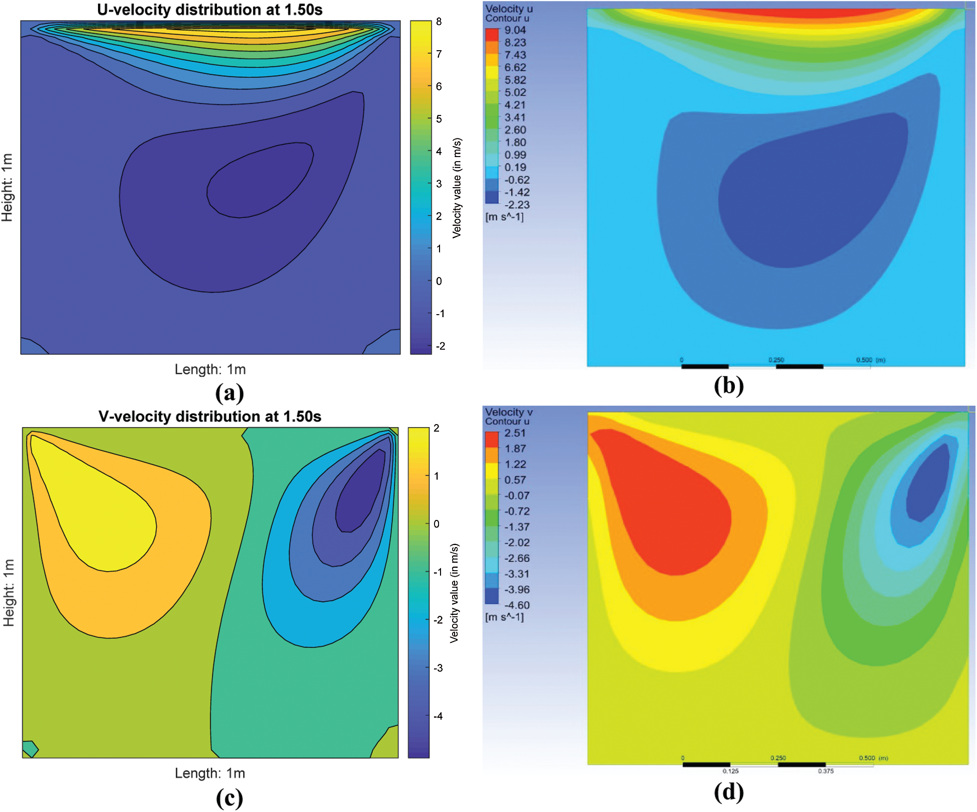
Figure 2: Comparison of contour plots at t = 1.50 s: (a) u-velocity using FDM MATLAB® and (b) FEM Ansys Fluent® (c) v-velocity using FDM MATLAB® and (d) FEM Ansys Fluent®

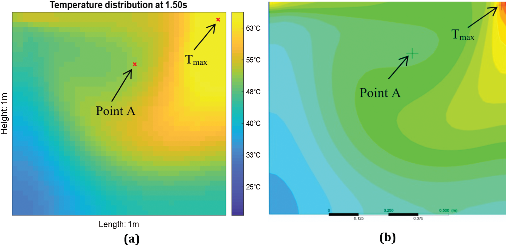
Figure 3: Comparison of image plot at t = 1.50 s (a) using FDM MATLAB® and (b) FEM Ansys

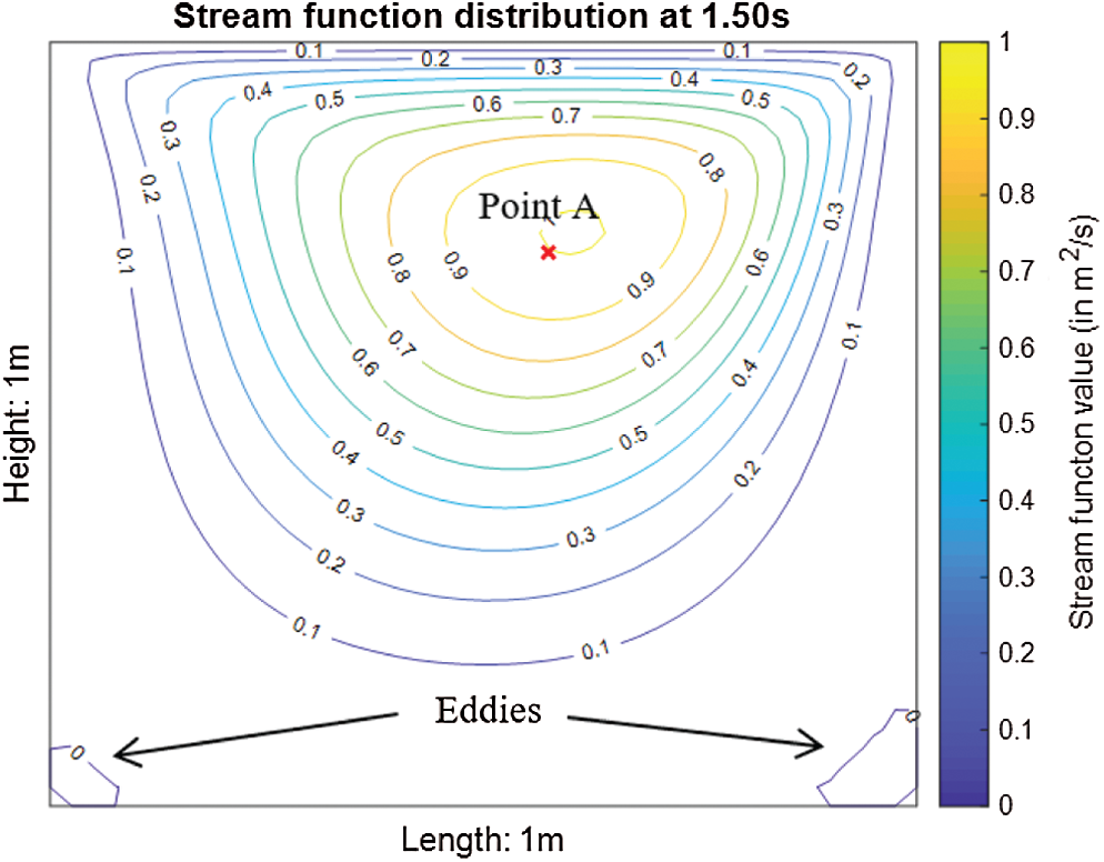
Figure 4: Stream function distribution at t = 1.50 s

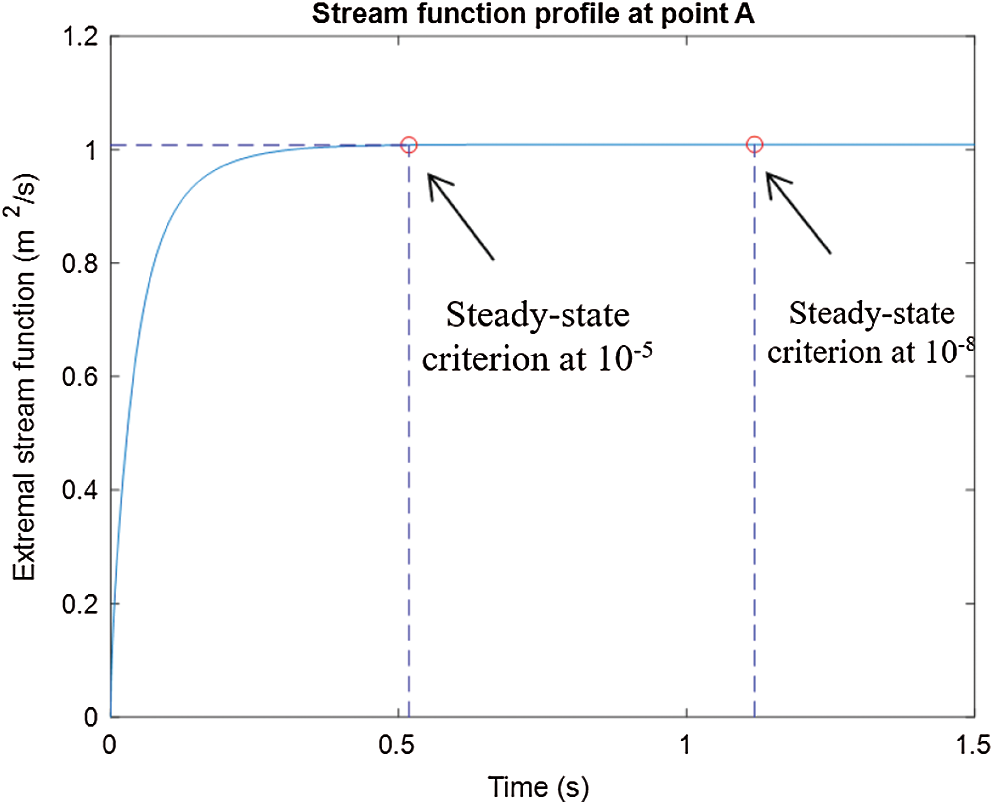
Figure 5: Stream function profile at the point A

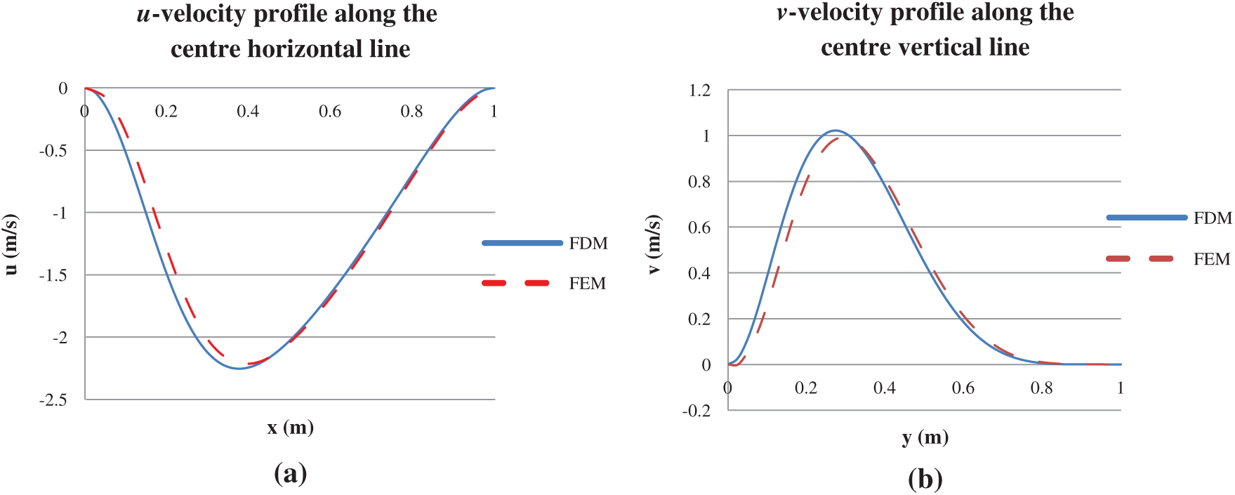
Figure 6: Comparison of results for (a) the u-velocity profile and (b) the v-velocity profile

Stream function, temperature distribution and location of the maximum temperature, Tmax for the 2nd test case are shown in Fig. 7. Besides, the associated contour plots of u- and v-velocity distributions of the cavity flow are shown in Fig. 8. Based on Figs. 3a and 7b, the temperature distributions are quite similar in both no-slip (1st test case) and free-slip (2nd test case) BCs. The heat is generated from the moving top lid and concentrated at the top right corner first. Subsequently the heat is slowly propagated to the right bottom corner and to the entire cavity. However, the overall temperature distribution is lower when the lid-driven flow is subject to the free-slip BC in Fig. 7b (2nd test case). Formation of eddies in the free-slip BC is also restricted in contrast with the no-slip BC (1st test case) as depicted in Fig. 7a. Comparison of temperature profiles at the point A for both test cases is shown in Fig. 9.

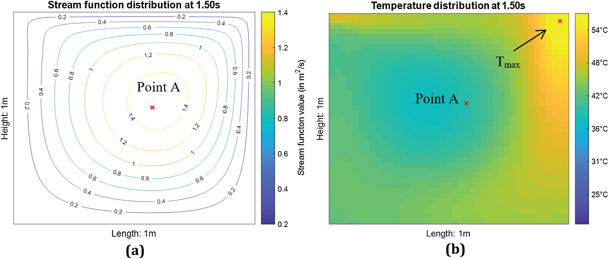
Figure 7: (a) Stream function and (b) temperature distribution for the 2nd test case (free-slip BC)

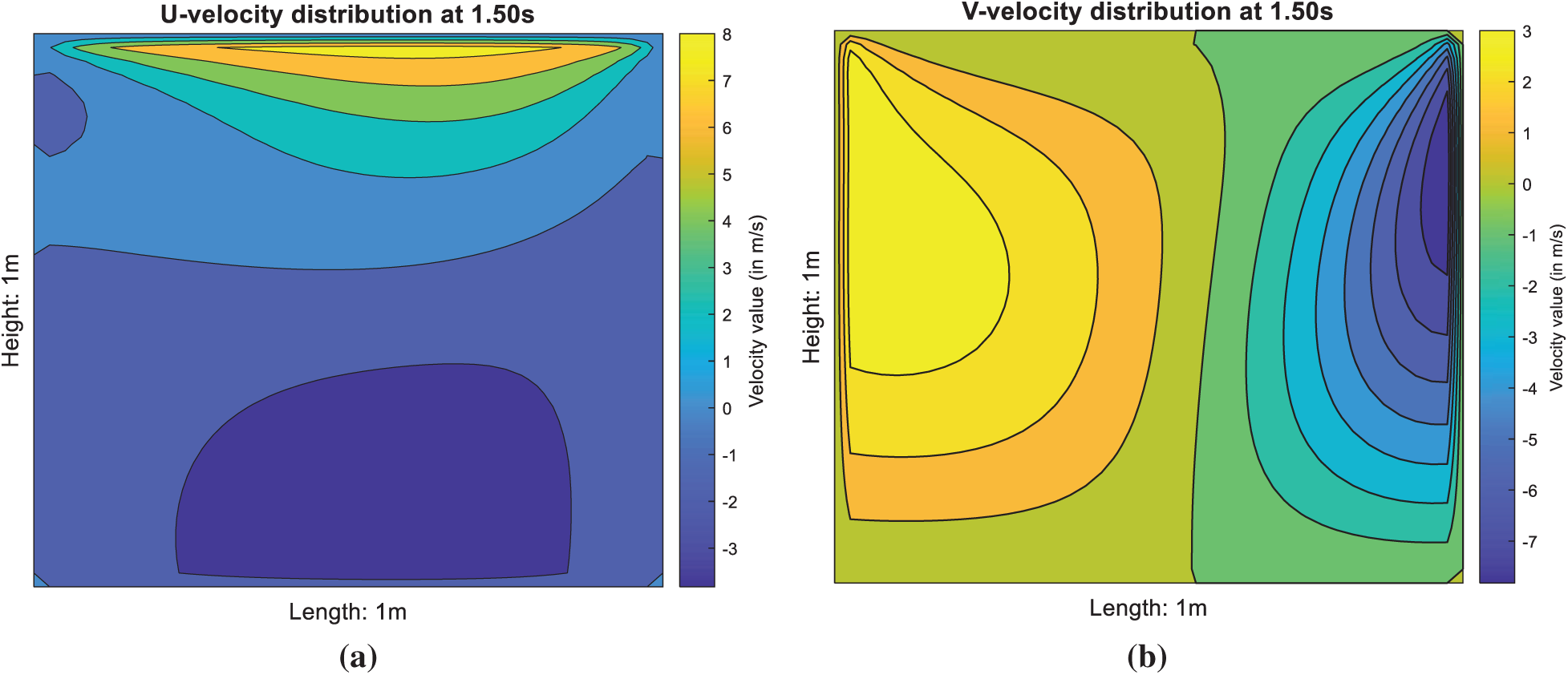
Figure 8: (a) U-velocity and (b) V-velocity distributions for the 2nd test case (free-slip BC)

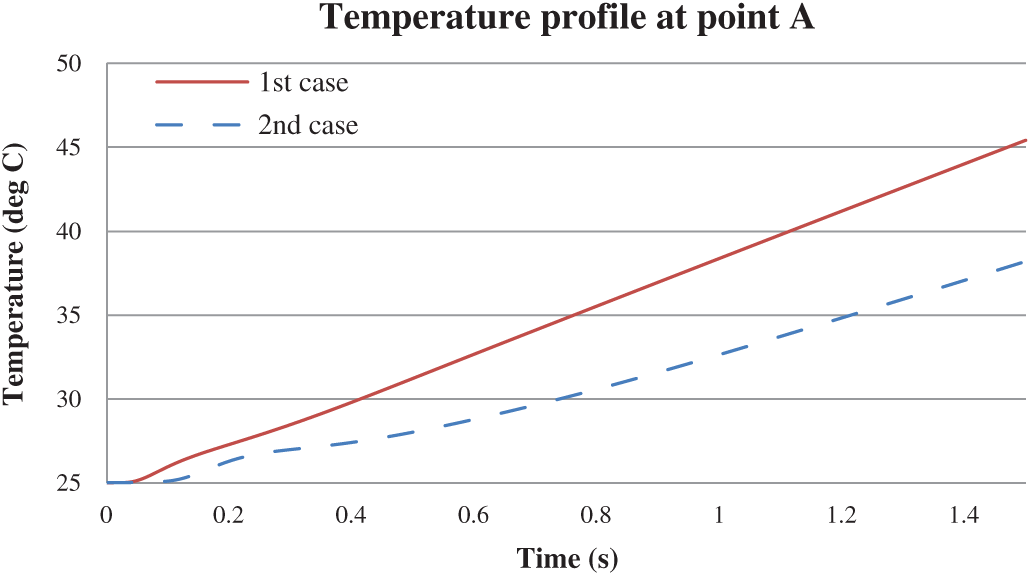
Figure 9: Temperature profile at the point A: (a) 1st test case (no-slip) and (b) 2nd test case (free-slip)

Both slip BCs show similar trend in temperature profile at the point A (location of maximum stream function, ψmax as shown in Figs. 3 and 7) and the temperatures keep increasing, but the no-slip BC gives an upper offset than the free-slip BC as shown in Fig. 9. This is due to the free-slip of the fluid at the wall or solid interface, thus no frictional heat can be generated at the wall. These two benchmarks (1st and 2nd test cases) are then compared with the 3rd and 4th test cases (with lower Reynold number, ReL than those benchmarks) as shown in Fig. 10. The 3rd and 4th cases show a reduction in temperature profile due to the lower value of applied velocity, Uwall which leads to a smaller stream function distribution in the whole lid-driven flow as prescribed by Eqs. (5) and (6). Because of the last term on the right-hand side of thermal energy equation in Eq. (12), the viscous heating term is much related to the stream function, ψmax and the resultant viscous heating will bring about a reduction in the temperature profile T(ψmax) at the point A. The benchmarks (the 1st and 2nd test cases) are then compared with the 5th and 6th test cases (with higher Prandtl number, Pr than those benchmarks) as shown in Fig. 11 for the temperature profile at the point A. All the results of the 1st until the 6th test cases are shown in Tab. 2.

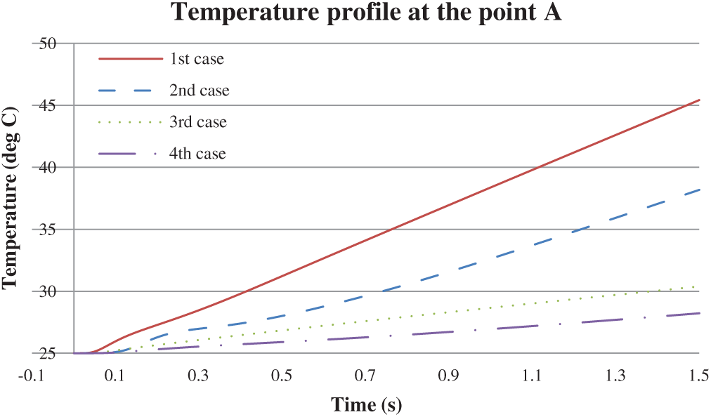
Figure 10: Temperature profile at the point A (ReL=100 vs. ReL=50)

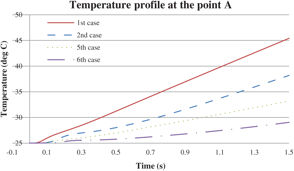
Figure 11: Temperature profile at the point A (Pr=1 vs. Pr=2)

Both the test cases (no-slip and free-slip BCs) show lower temperature profiles at the point A as compared to the benchmarks. Since Pr is directly proportional to specific heat, c, a higher value of c will result in a reduction of thermal boundary layer thickness. Recall that Prandtl number, Pr is a ratio of momentum and energy transport by diffusion in the velocity and thermal boundary layers given by [25]:

Pr=δδt,(34)

where δ is thickness of the velocity boundary layer and δt is thickness of the thermal boundary layer. It is also noticeable that the steady-state period at the criterion of e = 10−5 for the 5th and 6th test cases are similar with the benchmarks. Although the fluid flow has attained its steady-state condition as elucidated in Fig. 5, no steady-state condition can be observed in the temperature profiles of all the test cases as shown in Figs. 10 and 11. Moreover, temperature profile increases in quasi-linear behaviour even though Eq. (13) is an elliptic equation [32] due to the moving top lid provides an additional finite heat flux to the entire cavity. It can also be deduced that the temperature profile at the point A (or even at any point inside the cavity) will keep increasing if the iteration is extended at any period. The 1st test case is executed at the unsteady-state condition for 3 s as shown in Fig. 12 and it proves that the temperature profile is increasing quasi-linearly. This temperature rise is due to each of the fluid layers is being sheared relative to each other and this will create viscous heating caused by the fluid viscosity. The heat is being trapped inside the cavity flow by the insulated walls with no way to escape. Thus, temperature profile at every point inside the cavity flow (or temperature distribution of the cavity flow) will keep increasing. Based on Tab. 2, location of the maximum stream function, ψmax (point A) at the end of the iteration is merely influenced by Reynold number, ReL and free-slip BC whereas there is nothing to do with thermal conductivity, k and specific heat, c of the fluid. This is because solution of the stream function, ψ from Eq. (23) can be done without consideration of Eq. (25). Also, the location of the maximum temperature, Tmax at the end of the iteration is constant for all the test cases.

Table 2: Results of six test cases

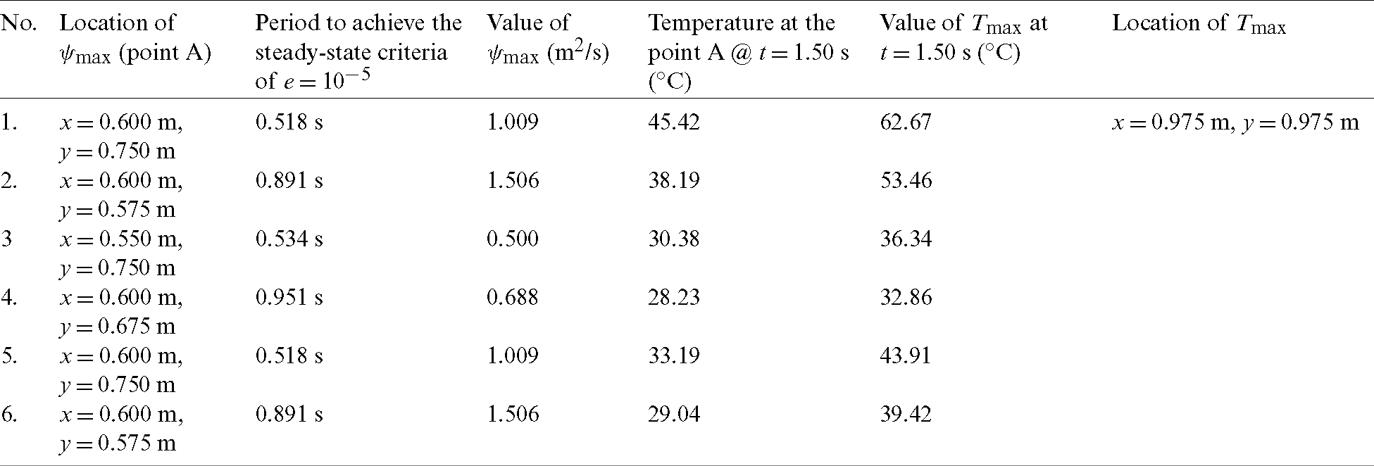
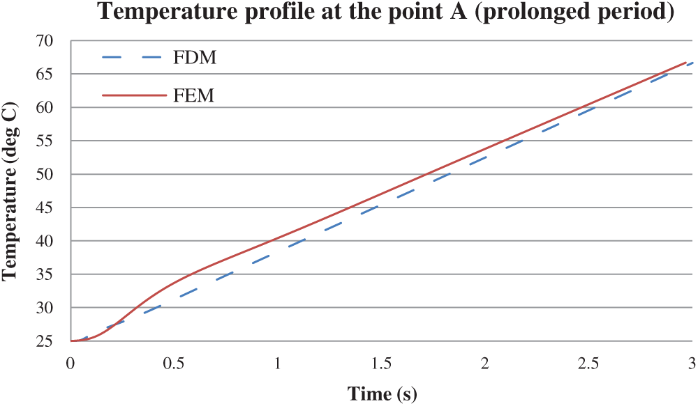
Figure 12: Temperature profile at the point A (1st test case at prolonged period)

5  Conclusion

In our study, we assume the two-dimensional unsteady lid-driven cavity model is perfectly insulated and no heat loss from the heat flux (viscous heating) is produced by the moving top lid to the environment. The FDM MATLAB solutions are verified earlier with FEM Ansys Fluent® before the six test cases are examined based on no-slip and free-slip BCs. The main findings are as follows:

•    Temperature profile shows an increasing trend in all test cases as the produced constant heat flux is supplied continuously by the moving top lid. If the iteration period is prolonged to any other period, the temperature profiles of these test cases will keep increasing. This is the reason why the surface temperature of a meteorite during its free-fall keeps increasing although the frictional heating or viscous heating due to the atmospheric air contributes a very small portion of heat.

•    Neumann BC is able to trap the heat produced inside the cavity model as the temperature profiles keep increasing quasi-linearly. Trapped heat is important for energy efficiency such as for building insulation during winter season.

•    The lower value of Reynolds number, ReL, the lower value of thermal diffusivity, α and the free-slip effect of the fluid flow can create lower temperature distributions.

•    Greater value of Prandtl number, Pr can reduce the temperature distribution inside the cavity model.

•    Free-slip effect will cause the fluid to flow faster but with a lower temperature distribution than that of the no-slip BC as the free-slip effect is assumed to act like a lubricant.

•    Although FDM scheme is simple and sufficient to explain the phenomenon of Neumann BC and free-slip effect, this method is limited to simple geometry only.

Funding Statement: The authors acknowledged the funding received from the Ministry of Higher Education, Malaysia and University of Malaya (https://umresearch.um.edu.my/) under the Project No: IIRG006C-19IISS leaded by Z. Siri for this study.

Conflicts of Interest: The authors declare no conflicts of interest to report regarding the present study.

This work is licensed under a Creative Commons Attribution 4.0 International License, which permits unrestricted use, distribution, and reproduction in any medium, provided the original work is properly cited.