Computers, Materials & Continua DOI:10.32604/cmc.2021.016123
Article

A Fault-Handling Method for the Hamiltonian Cycle in the Hypercube Topology

Adnan A. Hnaif*, Abdelfatah A. Tamimi, Ayman M. Abdalla and Iqbal Jebril

Faculty of Science and Information Technology, Al-Zaytoonah University of Jordan, Amman, 11733, Jordan
*Corresponding Author: Adnan A. Hnaif. Email: adnan_hnaif@zuj.edu.jo
Received: 24 December 2020; Accepted: 26 January 2021

Abstract: Many routing protocols, such as distance vector and link-state protocols are used for finding the best paths in a network. To find the path between the source and destination nodes where every node is visited once with no repeats, Hamiltonian and Hypercube routing protocols are often used. Nonetheless, these algorithms are not designed to solve the problem of a node failure, where one or more nodes become faulty. This paper proposes an efficient modified Fault-free Hamiltonian Cycle based on the Hypercube Topology (FHCHT) to perform a connection between nodes when one or more nodes become faulty. FHCHT can be applied in a different environment to transmit data with a high-reliability connection by finding an alternative path between the source and destination nodes when some nodes fail. Moreover, a proposed Hamiltonian Near Cycle (HNC) scheme has been developed and implemented. HNC implementation results indicated that FHCHT produces alternative cycles relatively similar to a Hamiltonian Cycle for the Hypercube, complete, and random graphs. The implementation of the proposed algorithm in a Hypercube achieved a 31% and 76% reduction in cost compared to the complete and random graphs, respectively.

Keywords: Hamiltonian cycle; hypercube; fault tolerance; routing protocols; WSN; IoT

1  Introduction

State-of-the-art technology, especially the Internet of Things (IoT), has increased the demand for Wireless Sensor Networks (WSNs). A WSN is a network of nodes that communicate with each other, sense the environment, and transmit the collected data via wireless links. A sensor network employs small, lightweight, battery-powered devices, known as sensor nodes [1–4]. In WSNs, each sensor node is equipped with a wireless communication module. The goal of sensor networks is to monitor a specific type of data within a particular area. For example, a sensor network can monitor the humidity, the temperature of the surrounding area, fire hazard, traffic status, or wildlife habitat [5–8]. Several routing algorithms, such as distance vector and link-state routing protocols [9,10], may be used to connect the nodes of the network, or [11] to connect the nodes of the ad hoc network.

Although WSNs can successfully distribute data collection for IoT applications, they have limited reliability because one or more nodes may become faulty [12] or need to be secured [13]. A sensor network may fail to monitor the surrounding area adequately due to the failure of some modules (such as the presence of factory defects in the sensor units), environmental factors, or battery power depletion. These failures will inevitably lead to a breakdown in the data transmission process between the source and the destination nodes and compromise the quality of service of the entire network [14].

Furthermore, the nature of the region plays an essential role in the distribution of sensors and may increase repair challenges. For example, a geographic territory with steep terrain is not easily accessible for repairing faulty sensors. Therefore, a failure could lead to the partitioning of the network into disjoint blocks, and to changing the routing path.

The problem of a complete halt in any communication network occurs when no message can be delivered towards its destination due to faulty nodes. Consequently, no communication occurs through the sensor nodes until the network administrator takes exceptional action to handle the problem, which usually requires a long time. Hamiltonian and Hypercube Routing Protocols can be used to solve the faulty node problem and therefore have been used in many applications to avoid deadlock issues [15].

Hamiltonian routing protocols employ either a Hamiltonian path or a Hamiltonian cycle. The Hamiltonian path requires visiting each node of the graph exactly once during the routing process. When the end node is the same as the start node, it becomes a Hamiltonian cycle [6].

A Hypercube is either a graphical representation of some nodes and edges or is the set of all n-bit strings denoted by {0,1}n in a single unit in any dimension n, which is called n-cube [16].

A complete graph, denoted by Kn, is a graph where n is the number of nodes with an edge that links each pair of separate nodes. The graph is assumed to be simple; i.e., it contains no loops or multiple edges.

A connected graph G is a graph where each pair of nodes is connected by a simple path.

This paper will present a modified Hamiltonian cycle protocol implemented on a Hypercube graph to find an alternative cycle in case of the occurrence of one or more faulty nodes. Additionally, a new simulator, called HNC, has been designed and implemented to verify the efficacy of this protocol.

The rest of this paper is organized as follows. Section 2 provides graph-theory preliminaries on the Hamiltonian path and cycle and Hypercube graphs. Section 3 reviews related works. In Section 4, the theorems lying behind the proposed algorithm are proven and the general idea of the algorithm is introduced and explained briefly. The algorithm and pseudo code of the algorithm’s components are given in Section 5, where the simulation results are shown in Section 6. Finally, Section 7 concludes the paper followed by the list of references.

2  Preliminaries

This section reviews and discusses some basic concepts and definitions of the Hamiltonian and Hypercube topologies.

Definition 1 (Hamiltonian Path): In a graph G, a Hamiltonian Path is a path that contains every node of G [17].

Definition 2 (Hamiltonian Cycle): In a graph G, a cycle c of G, which contains every node of G, is said to be a Hamiltonian cycle. In this case, G is called a Hamiltonian graph [18].

Definition 3 (Hypercube): A Hypercube, Q_n, is a graph whose node set V consists of the n-dimensional Boolean vectors, i.e., vectors with binary coordinates 0 or 1, where two nodes are adjacent whenever they differ in exactly one coordinate [6]. Fig. 1 shows an example of a 4-dimensional Hypercube.

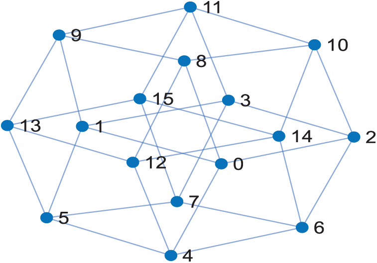
Figure 1: A 4-dimensional hypercube

Luca Trevisan [19] proved the following theorem.

Theorem 1: For every n≥2, the n-dimensional Hypercube has a Hamiltonian cycle.

Consequently, we propose solving the faulty node problem in the Hamiltonian cycle routing protocol for the Hypercube. Hypercube Qn with 2n nodes is an undirected graph where each node is labeled with a binary number that differs from each of its adjacent nodes in exactly one bit. The parity of the node is determined based on the number of 1’s in its binary-number label; i.e., the parity is 0 if the number of ones is even and otherwise it is 1.

The n-Hypercube graph also called the n-cube graph and commonly denoted as Qn or 2n, is the graph whose vertices are the 2k nodes ϵ1,…,ϵn where ϵi=0 or 1 and two vertices are adjacent if the nodes differ in exactly one coordinate.

In addition, Hypercube Qn is not Hamiltonian if all edges are going in one direction and of the same parity of faulty nodes. Consequently, [20] showed that the Hypercube is Hamiltonian if n≥4. Accordingly, there are two edges of different parity if Qn has n≥4 and is free of faulty nodes.

Hsieh et al. [21] presented two theorems. The first theorem verified that there exists a fault-free Hamiltonian path in an n-dimensional Mobius cube (denoted by MQn) with up to n-1 faulty nodes for n≥4. The second theorem showed that a fault-free cycle with a length between 4 and 2n faulty nodes can be tested in a faulty Mobius cube MQn with up to n-2 faulty nodes for n≥2.

In order to find the most extended cycle in an n-dimensional Hypercube graph G, [22] proposed a twisted Hypercube-like network (THLN) with up to 2n-9 faulty nodes (F). They showed that (G-F) contains a Hamiltonian cycle when (δ(G-F)>2) and (G-F) include a near Hamiltonian cycle given that (δ(G-F)≤1). Fig. 2 shows a 4-dimensional Hypercube with Hamiltonian cycle.

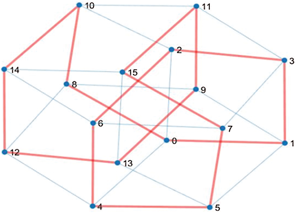
Figure 2: A 4-dimensional hypercube with Hamiltonian cycle

3  Related Work

This section discusses the traditional Hamiltonian cycle, Hamiltonian path, and Hypercube used to connect nodes. Ammerlaan et al. [18], proved that a Hamiltonian cycle exists between the kth and (n–k)th level of the n-dimensional Hypercube by using the Gray code counting system. To obtain the Gray code counting system, the exclusive-OR operation is computed between the consecutive bits of the corresponding binary number. Other researchers, like [20], implemented an algorithm to detect any Hamiltonian cycle in the cube. They considered an edge u a neighbor of an edge v if u and v are neighbors in Qn and the node (n,v)/∈F is healthy; otherwise, no Hamiltonian cycle is possible. Furthermore, [23] presented a theorem to ensure the existence of a Hamiltonian path in a graph. They assumed G=(V,E) to be a connected graph. For non-adjacent edges, there should be e(u) ande(v)=δ(c,v)≥n+1 and then G will have a Hamiltonian path.

Xiaofan et al. [24] described the properties of the Hypercube, where a single volumetric unit in any dimension is a Hypercube. All edges that meet at a node are perpendicular to each other. A unique digit of length ‘n’ could label each node if the Hypercube is positioned in the origin of the coordinate system. The number of nodes resulting in a unique binary word is equivalent to the possible binary strings of length ‘n’ and can be calculated as the number of nodes=2n. Likewise, [24] designed a layered structure of a Hypercube graph and noted that each corresponding string (node) can be grouped based on the number of ones. Any edge connects two or more nodes if the difference between the nodes is only one bit. (ni) can be used to calculate the ith number of nodes, and between node layers i andi+1 there exists an edge layer containing (ni+1)(n-i), or equivalently, (ni)(i+1) edges.

Guo et al. [25] devised a new condition of diagnosability to enhance the diagnosability issue. The conditional diagnosability implies that not all neighbors of any edge fail at the same time. Similarly, they proposed that any system is called conditionally t-diagnosable when each pair of the set of the faulty nodes (F0, F1) is distinguishable for |F|≤t and proved that tc(EH(s,t))=3s-2 for t≥s>2.

Zhang et al. [22] proposed an architecture called THLN for several multiprocessor systems using Hamiltonian connectivity, based on twisted Hypercube-like networks to improve the communication cost between processors. In addition, they proved that the graph G is an n-dimensional THLN for n≥5 and F is a subset of V(Gn)∪E(Gn) with |F|. Moreover, they showed that for the node pair (u,v) in the graph Gn-F, there exists an (n-2) fault-tolerant Hamiltonian path, except for (u,v) because it is a weak node-pair in Gn-F.

Liu et al. [26] proved two theorems for the n-dimensional twisted Hypercube Hn. The first theorem proved that Hn has a fault-free Hamiltonian cycle if the number of the faulty nodes >n-2. The second theorem proved that Hn has a faulty open Hamiltonian path if the number of faulty nodes >n-3 for any pair of non-faulty nodes. Nikolaev et al. [27] introduced an algorithm to find a Hamiltonian decomposition of the 4-regular multigraph called the variable neighborhood search (VNS) algorithm. The main objective of VNS is to solve the traveling salesperson problem. For nonadjacent nodes, given two Hamiltonian cycles: x and y, if the graph G(x∪y) contains a Hamiltonian decomposition into node-disconnect cycles z and w different from x and y, then the corresponding nodes xu and yu are not adjacent.

Chen [28] considered the problem of existing faulty nodes in the Hamiltonian cycle that contains a direct link connection between nodes and avoids the faulty nodes in an n-cube Qn. The author showed that all edges of the matching node M lie on a fault-node-free Hamiltonian cycle in Qn if Qn contains 2n-4-|M| faulty edges and the maximum allowed number of faulty edges is sharp when |M|=1 or |M|=2.

4  Modified Hamiltonian Cycle Based On Hypercube Topology

Theorem 2: Let G be a Hypercube graph with a degree (n≥2). If A, B, and C are nodes in G, then there exists at least one Hamiltonian path from A to C through B* where B*∈G and B*≠B.

Let G(V,E,w) be a Hypercube graph, where V is the union of all ith node {vi,j},j=1,2,3,…,(ni). The set of nodes in the ith layer can be assigned as shown by Eq. (1)

vi={vi,j}j=1(ni)(1)

Let E⊆V×V be the set of edges and ‘w’ be the function that assigns a non-negative weight w to every edge. Then, the number of edges from any vi,j node will be w(vi,j,v*) where v* can be calculated by Eq. (2)

v*={{v1,ik}k=1n,if vi,j=v0,1,{vi-1,jk}k=1i∪{vi+1,jk}k=1n-iifvi,j≠v0,1orvi,j≠vn,1,{vn-1,jk}k=1n,ifvi,j=vn,1.(2)

In general, the number of all edges in the ith node layer of a Hypercube contains an (ni)(n-1) edge layer.

Proof: Let A=vi,j∈v then:

Case 1: See Eq. (3)

A=v0,1∈v(3)

and since (n≥2) then there is at least (See Eq. (4))

B*∈{v0,j}nj=1\{v0,1}(4)

Such that B*≠Bandw(A,B*) exist.

Case 2: See Eq. (5)

A=vn,1∈v(5)

and since (n≥2) then there is at least (See Eq. (6))

B*∈{vn,j}nj=1\{vn,1}(6)

Such that B*≠Bandw(A,B*) exist.

Case 3: See Eq. (7)

A≠v0,1andA≠vn,1(7)

and since (n≥2) then there is at least (See Eq. (8))

B*∈{vi-1,jk}ik=1∪{vi+1,jk}n-1k=1≠ϕ(8)

Such that B*≠Bandw(A,B*) exist.

Consequently, there exists at least one Hamiltonian path from node A to node C through node B where w(A,B*) and w(B*,C) exist.

To introduce our own proposed algorithm (FHCHT) based on the above theorems, Fig. 3 depicts the flowchart of the proposed modified Hamiltonian Cycle based on Hypercube Topology.

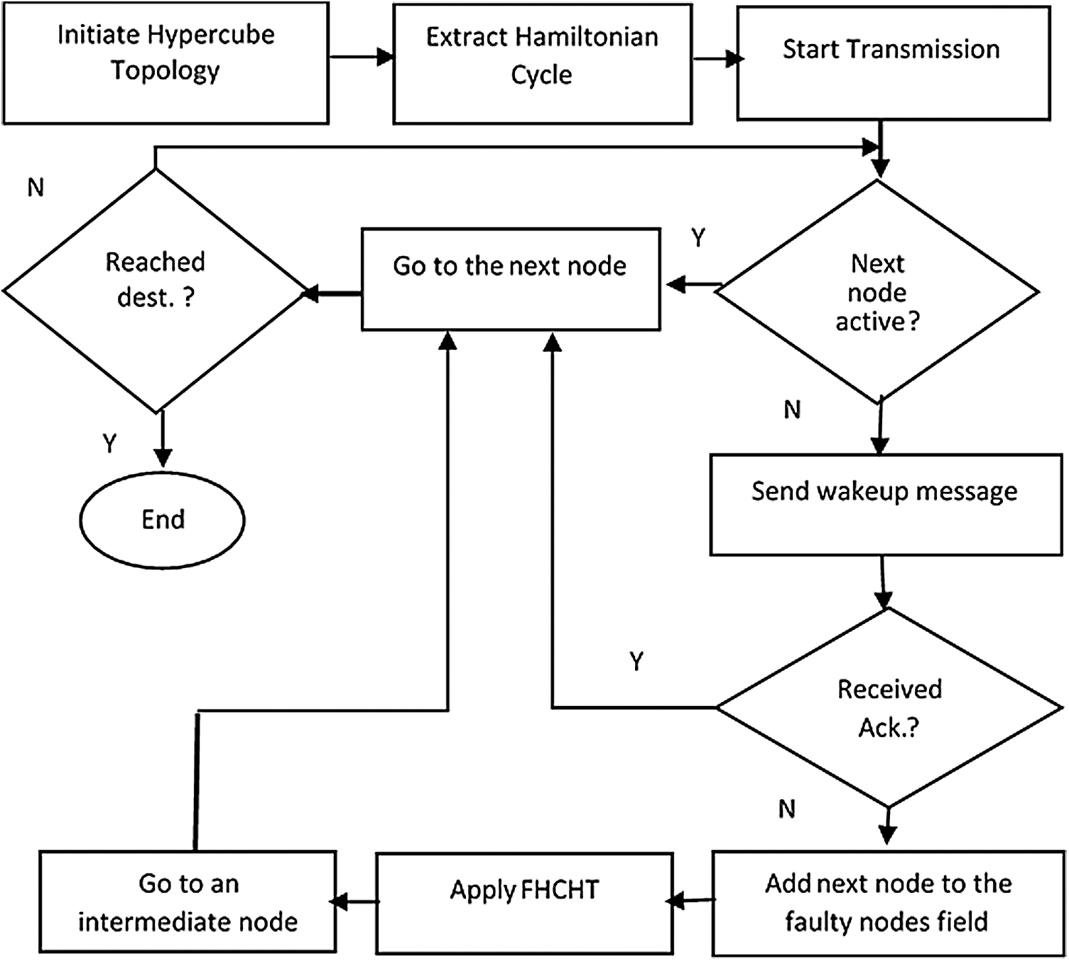
Figure 3: A flowchart of the proposed FHCHT algorithm

To reduce the cost of transmission and avoid existing faulty nodes, the Hamiltonian cycle is used first to label all nodes and to process the communication between nodes. This phase is called the initialization phase. As mentioned, the Hamiltonian cycle algorithm is used where the source address is the same as the destination address (start node = destination node). At this phase, all nodes are labeled either in binary or in decimal and the transmission phase is applied, which has two scenarios. The first scenario is called the standard scenario where the packet is transmitted smoothly from the source node to the destination node using the Hamiltonian cycle without any obstacles. The second scenario is when one or more nodes do not work (faulty node). Here, FHCHT is applied to bypass these nodes and go to the next node through an intermediate node, and to find other possible paths.

5  Algorithms of the System

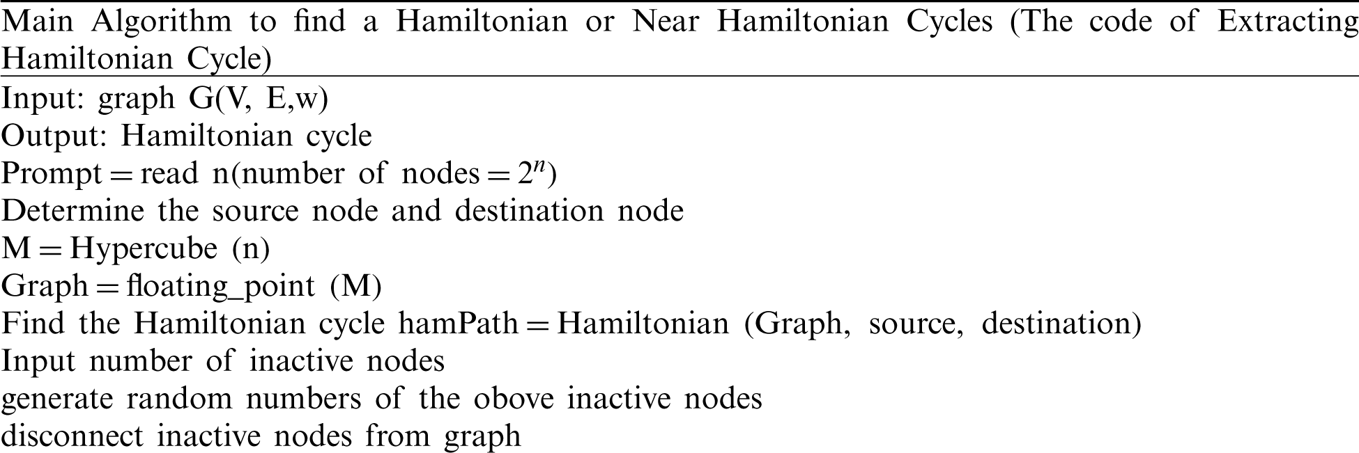
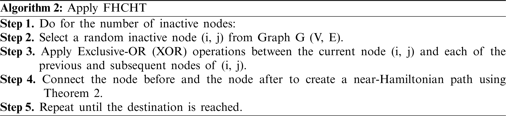
In this section, we introduce the two proposed algorithms: Extracting Hamiltonian Cycle and Applying FHCHT.

5.1 Extracting Hamiltonian Cycle

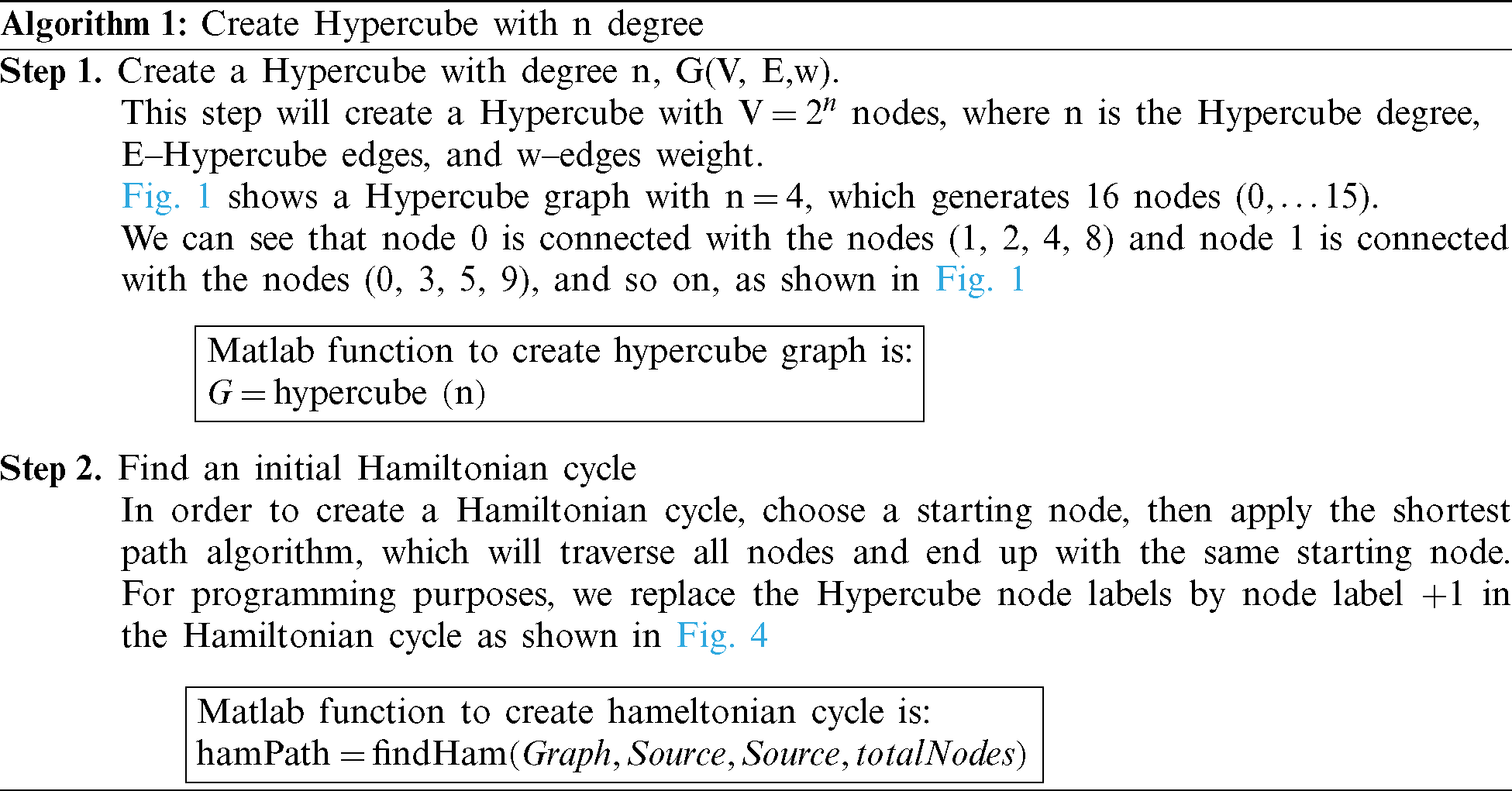
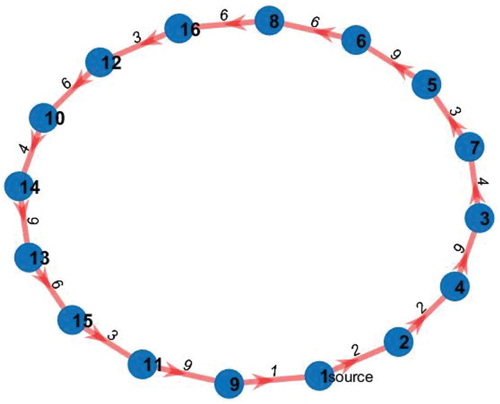
Figure 4: Initial Hamiltonian cycle

The code of the algorithm is as follows:

5.2 Applying FHCHT

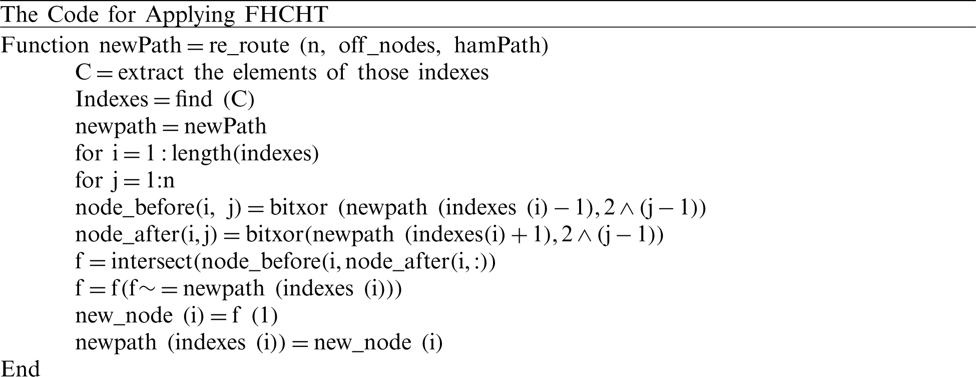
The code for applying the algorithm is as follows:

Figs. 5–7 show a near-Hamiltonian cycle with 1, 2 and 3 faulty nodes respectively.

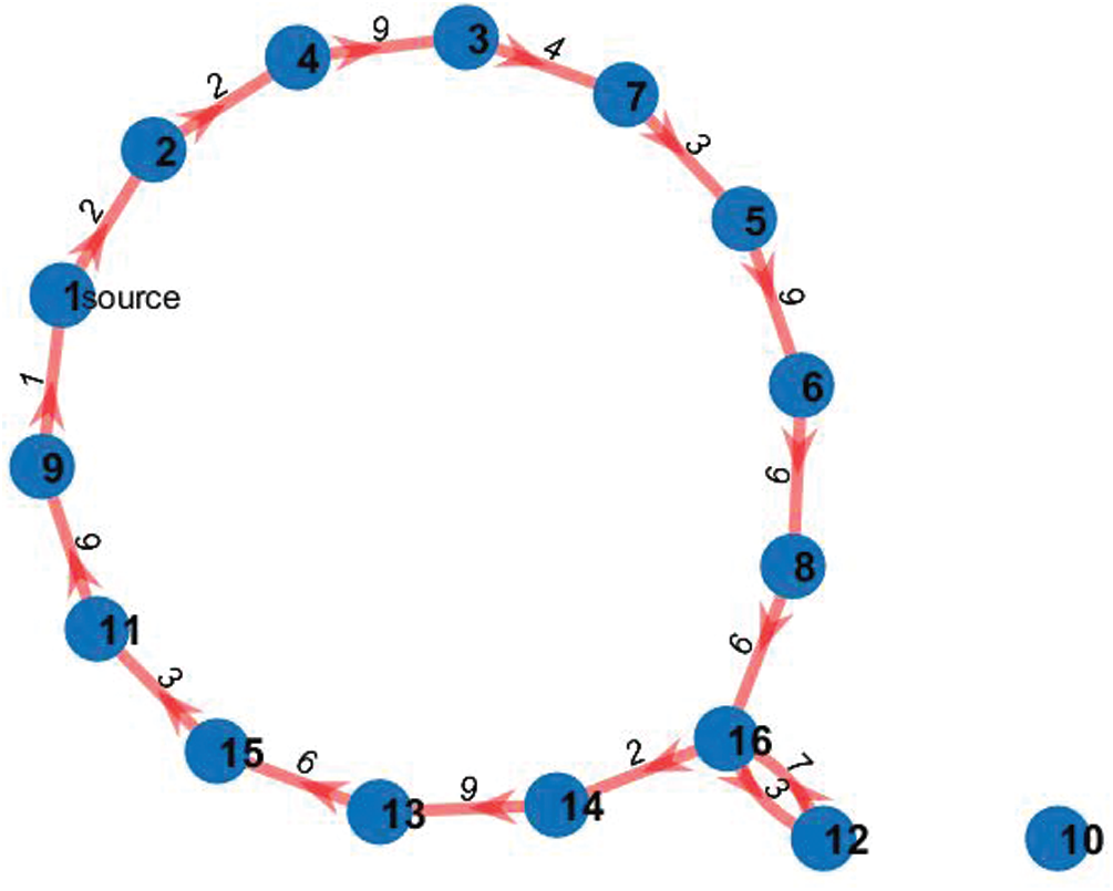
Figure 5: A near-Hamiltonian cycle with one inactive node

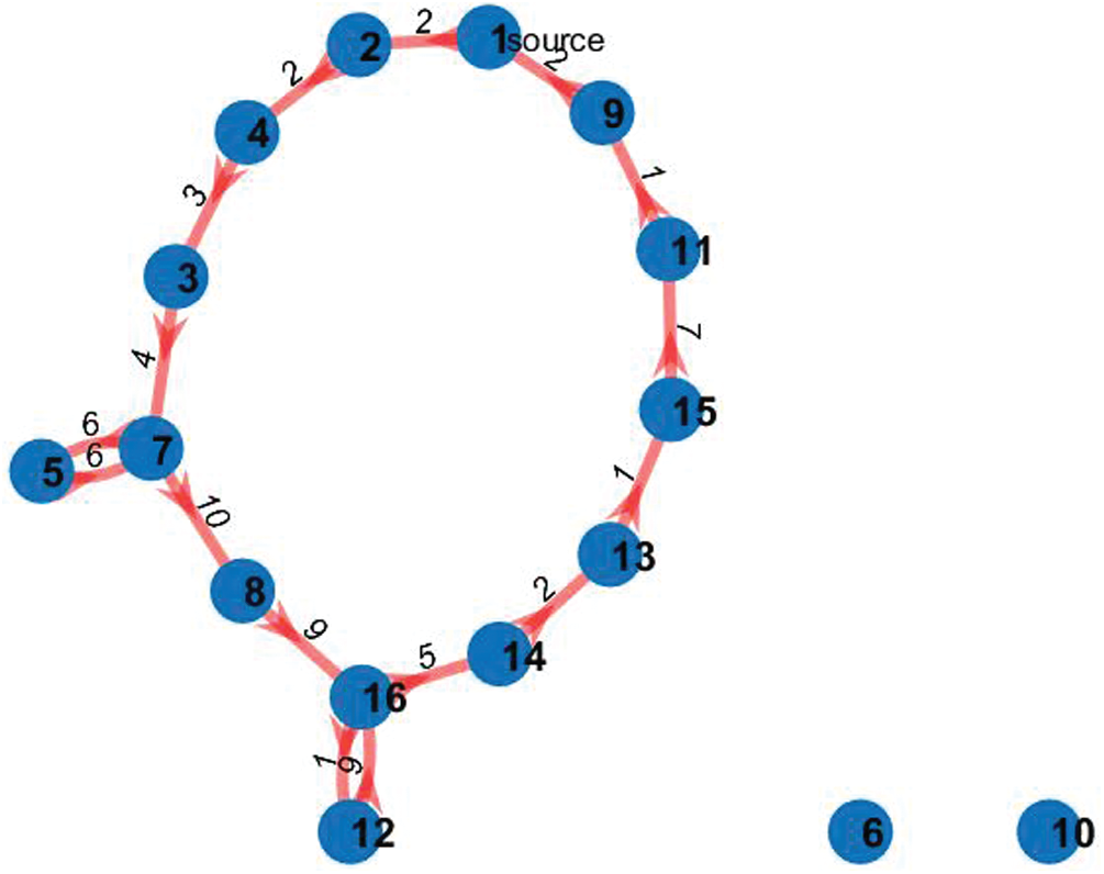
Figure 6: A near-Hamiltonian cycle with two inactive nodes

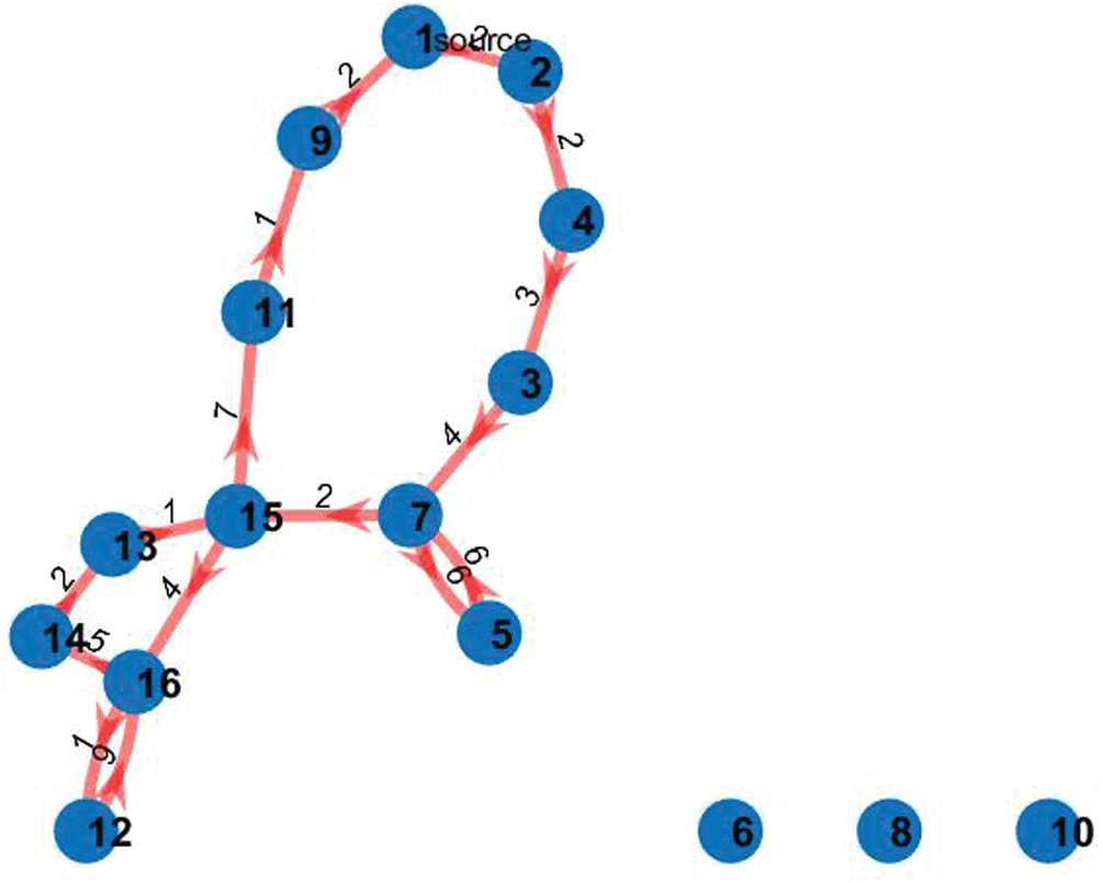
Figure 7: A near-Hamiltonian cycle with three inactive nodes

6  Experimental Results and Analysis

In this section, we introduce the implementation of the proposed FHCHT algorithm and show the obtained simulation results. The simulation was run with Matlab 2019 on a laptop computer with Intel Core i5 Duo CPU 2900 4M, 4GB DDR3 RAM, and Windows 10 operating system.

As an example, let a Hypercube degree (n=4) and therefore the number of nodes will be 24 = 16, as illustrated in Fig. 1. The first step is the initialization of the Hypercube topology and then the extraction of the Hamiltonian cycle is applied. See Figs. 2 and 4, respectively, where a packet runs through the highlighted path (depicted in red).

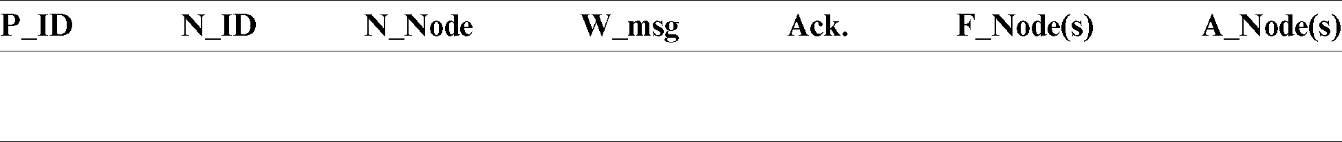
The packet format is shown in Tab. 1. The input data of Tab. 1 are listed below.

P_ID: packet ID, N_ID: Node ID, N_Node: Next Node, W_msg: Wakeup Message, Ack.: Acknowledgment, F_Nodes: Faulty Node(s) and A_Nodes: Alternative Node(s).

Table 1: Packet format

To find a near-Hamiltonian path after a faulty node(s) exists, apply Algorithm 2. If a full Hamiltonian cycle exists, then it exits and outputs the Hamiltonian cycle with no faulty nodes. Otherwise, the output is a near-Hamiltonian cycle with one or more loops.

To increase the efficiency of the system, the source node will use Tab. 2 for reference to avoid the faulty nodes in the subsequent routes when no updates are available.

Table 2: Source reference information

A subcase example is shown in Fig. 4. In this example, suppose that node 4 and node 5 become faulty. Consequently, node 2 will send a wakeup message to node 4 and wait to receive an acknowledgment. If the acknowledgment is received, then go to node 4; otherwise, node 4 will be added to the faulty node field, and FHCHT will be applied to find an alternative path from node 2 to node 3.

Additionally, we implemented a complete connected and random connected graphs with node degree greater than or equals 2, in order to compare the efficiency and total cost, when we obtain a Hamiltonian or near-Hamiltonian cycle. Fig. 8 depicts the complete graph with a Hamiltonian cycle. graph with two faulty nodes (node 4 and 5).

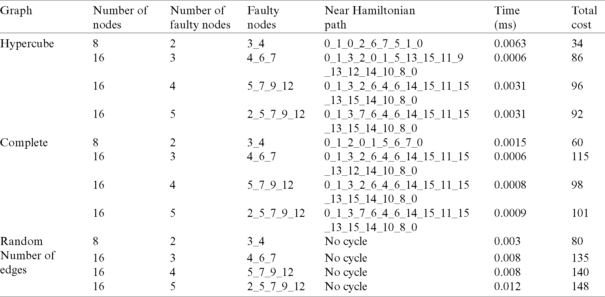
Tab. 3 compares the results between a Hypercube, complete, and random graphs based on the number of nodes, the number of faulty nodes, and the name of faulty nodes, where all faulty nodes are selected randomly. The simulator was run on 8 and 16 nodes. For the simulation with 16 nodes, the execution was repeated with three different numbers of faulty nodes–nodes 3, 4, and 5 for all graphs.

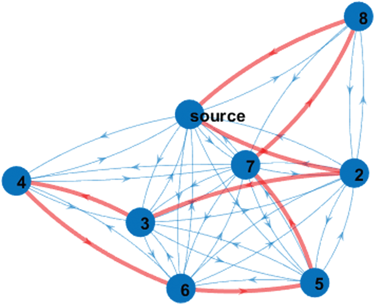
Figure 8: The complete graph with a Hamiltonian cycle

Table 3: A comparison between the results of the Hypercube, completed, and random graphs

By applying Algorithm 2 twenty times with a fixed number of nodes with randomly generated faulty nodes, we got the results shown in Tab. 4, where the number of graph edges in the Hypercube is equal to n*2n-1 and the number of edges in the complete graph equals (2n(2n −1)/2), where n is the Hypercube degree.

Table 4: A comparison between the results of hypercube, completed, and random graphs based on the number of the randomly generated faulty nodes

The results show that the time required for the complete graph was better than the time of the Hypercube, while the cost for the complete graph, measured by the number of edges, is greater than in the Hypercube. For instance, for a Hypercube with 16 nodes, the number of edges is 32, while in the complete graph for the same number of nodes the number of edges is 120, which was a significant difference between them.

At the same time, when we use a graph with a random number of edges to reduce cost, we cannot guarantee an existing Hamiltonian or near-Hamiltonian cycle. Thus, it is not preferable to choose a random number of edges.

7  Conclusion

In this study, a Modified Fault-free Hamiltonian cycle based on the Hypercube Topology (FHCHT) and a Hamiltonian Near Cycle (HNC) simulator were developed to obtain one or more alternative paths between the source and the destination nodes in WSNs. FHCHT aims to solve a well-known faulty node problem. HNC was applied as follows. First, Hypercube connectivity was used to establish a connection path between the source and destination through a set of active nodes. Second, a random number was chosen to represent the number of faulty nodes. Third, HNC was applied to create and find the shortest path.

The results obtained from HNC confirmed that the proposed algorithm finds multiple alternative paths between the source and destination nodes with the existence of many faulty nodes with an approximate 31% reduction of cost over the complete graph and a 76% reduction over the random graph. However, repeated runs for a Hypercube, complete and random graphs show that the Hypercube edges are fewer than the complete graph edges, which reduces the connection cost. Meanwhile, the random connected graph does not guarantee to obtain a Hamiltonian or near Hamiltonian cycle when a number of faulty nodes exist. The rectified communication process should enhance the overall efficacy of WSN applications.

Acknowledgement: The authors would like to thank Al-Zaytoonah University of Jordan for supporting this research.

Funding Statement: The author(s) received no specific funding for this study.

Conflicts of Interest: The authors declare that they have no conflicts of interest to report regarding the present study.

References

 1.  O. I. Khalaf, G. M. Abdulsahib and B. M. Sabbar. (2020). “Optimization of wireless sensor network coverage using the bee algorithm,” Journal of Information Science and Engineering, vol. 36, no. 2, pp. 377–386. [Google Scholar]

 2.  S. K. Prasad, J. Rachna, O. I. Khalaf and D. N. Le. (2020). “Map matching algorithm: Real time location tracking for smart security application,” Telecommunications and Radio Engineering, vol. 79, no. 13, pp. 1189–1203. [Google Scholar]

 3.  A. D. Salman, O. I. Khalaf and G. M. Abdulsahib. (2019). “An adaptive intelligent alarm system for wireless sensor network,” Indonesian Journal of Electrical Engineering and Computer Science, vol. 15, no. 1, pp. 142–147. [Google Scholar]

 4.  O. I. Khalaf and G. M. Abdulsahib. (2019). “Frequency estimation by the method of minimum mean squared error and P-value distributed in the wireless sensor network,” Journal of Information Science and Engineering, vol. 35, no. 5, pp. 1099–1112. [Google Scholar]

 5.  A. A. A. Alkhatib, M. Alia and A. Hnaif. (2017). “Smart system for forest fire using sensor network,” International Journal of Security and Its Applications, vol. 11, no. 7, pp. 1–16. [Google Scholar]

 6.  Y. Kim, K. Bok, I. Son, J. Park, B. Leea et al. (2017). , “Positioning sensor nodes and smart devices for multimedia data transmission in wireless sensor and mobile P2P networks,” Multimedia Tools and Applications, vol. 76, no. 16, pp. 17193–17211. [Google Scholar]

 7.  N. Imran, S. Riaz, A. Shaheen, M. Sharif and M. Raza. (2014). “Comparative analysis of link-state and distance vector routing protocols for mobile ad hoc networks,” Science International (Lahore), vol. 26, no. 2, pp. 669–674. [Google Scholar]

 8.  O. I. Khalaf and B. M. Sabbar. (2019). “An overview on wireless sensor networks and finding optimal location of nodes,” Periodicals of Engineering and Natural Sciences, vol. 7, no. 3, pp. 1096–1101. [Google Scholar]

 9.  O. I. Khalaf and G. M. Abdulsahib. (2020). “Energy efficient routing and reliable data transmission protocol in WSN,” International Journal of Advances in Soft Computing and Its Application, vol. 12, no. 3, pp. 45–53. [Google Scholar]

10. A. F. Subahi, Y. Alotaibi, O. I. Khalaf and F. Ajesh. (2020). “Packet drop battling mechanism for energy aware detection in wireless networks,” Computers, Materials & Continua, vol. 66, no. 2, pp. 2077–2086. [Google Scholar]

11. N. Sulaiman, G. Abdulsahib, O. Khalaf and M. N. Mohammed. (2014). “Effect of using different propagations of OLSR and DSDV routing protocols,” in Proc. of the IEEE Int. Conf. on Intelligent Systems Structuring and Simulation, Langkawi, Malaysia, pp. 540–545. [Google Scholar]

12. M. T. Lazarescu. (2017). Wireless Sensor Networks for the Internet of Things: Barriers and Synergies, In: G. Keramidas, N. Voros, M. Hübner (Eds.) Turin, Italy: Springer, Cham, . [Online]. Available: https://link.springer.com/chapter/10.1007/978-3-319-42304-3_9. [Google Scholar]

13. O. I. Khalaf, G. M. Abdulsahib, H. D. Kasmaei and K. A. Ogudo. (2020). “A new algorithm on application of blockchain technology in live stream video transmissions and telecommunications,” International Journal of e-Collaboration, vol. 16, no. 1, pp. 16–32. [Google Scholar]

14. O. I. Khalaf, G. M. Abdulsahib and M. Sadik. (2018). “A modified algorithm for improving lifetime WSN,” Journal of Engineering and Applied Sciences, vol. 13, no. 21, pp. 9277–9282. [Google Scholar]

15. A. A. Hnaif, A. el-Obaid and N. Al-ramahi. (2017). “Traffic light management system based on Hamiltonian routing technique,” Journal of Theoretical and Applied Information Technology, vol. 95, no. 1, pp. 2792–2802. [Google Scholar]

16. H. Park and J. W. Lee. (2012). “Task assignment and migration in wireless sensor networks via task decomposition,” Information Technology and Control, vol. 41, no. 4, pp. 340–348. [Google Scholar]

17. A. Mahasinghe, R. Hua, M. J. Dinneen and R. Goyal. (2019). “Solving the hamiltonian cycle problem using a quantum computer,” in Proc. ACSW, Association for Computing Machinery, New York, NY, United States, pp. 1–9. [Google Scholar]

18. J. Ammerlaan and T. S. Vassilev. (2013). “Properties of the binary hypercube and middle level graphs,” Applied Mathematics, vol. 3, no. 1, pp. 20–26. [Google Scholar]

19. L. Trevisan. (2007). “Discrete mathematics for CS. lecture 14,” . [Online]. Available: http://docplayer.net/38836783-Discrete-mathematics-for-cs-spring-2007-luca-trevisan-lectures-polynomials.html. [Google Scholar]

20. J. Dybizbański and A. Szepietowski. (2019). “Hamiltonian cycles and paths in Hypercubes with disjoint faulty edges,” arXiv preprint arXiv, vol. 2, pp. 1–12. [Google Scholar]

21. S. Y. Hsieh and N. W. Chang. (2006). “Hamiltonian path embedding and pancyclicity on the mobius cube with faulty nodes and faulty edges,” IEEE transactions on computers, vol. 55, no. 7, pp. 854–886. [Google Scholar]

22. H. Zhang, X. Xu, J. Guo and Y. Yang. (2018). “Fault-tolerant Hamiltonian connectivity of twisted hypercube-like networks THLNs,” IEEE Access, vol. 6, pp. 74081–74090. [Google Scholar]

23. M. S. Rahman and M. Kaykobad. (2005). “On Hamiltonian cycle and Hamiltonian path,” Information Processing Letters, vol. 94, no. 1, pp. 37–41. [Google Scholar]

24. X. Yang, Q. Dong, E. Yang and J. Cao. (2011). “Hamiltonian properties of twisted hypercube-like networks with more faulty elements,” Theoretical Computer Science, vol. 412, no. 22, pp. 2409–2417. [Google Scholar]

25. C. Guo, M. Leng, Z. Xiao and S. Peng. (2018). “Conditional diagnosability of exchanged hypercube under the MM* model,” IEEE Access, vol. 6, pp. 61151–61162. [Google Scholar]

26. H. Liu, X. Hu and S. Gao. (2019). “Hamiltonian cycles and paths in faulty twisted Hypercubes,” Discrete Applied Mathematics, vol. 257, no. 1, pp. 243–249. [Google Scholar]

27. A. Nikolaev and A. Kozlova. (2020). “Hamiltonian decomposition and verifying vertex adjacency in 1-skeleton of the traveling salesperson polytope by variable neighborhood search,” Journal of Combinatorial Optimization, vol. 218, pp. 1–13. [Google Scholar]

28. X. B. Chen. (2019). “Matchings extend to Hamiltonian cycles in Hypercubes with faulty edges,” Frontiers of Mathematics in China, vol. 14, no. 6, pp. 1117–1132. [Google Scholar]

This work is licensed under a Creative Commons Attribution 4.0 International License, which permits unrestricted use, distribution, and reproduction in any medium, provided the original work is properly cited.