DOI:10.32604/cmc.2021.016163
| Computers, Materials & Continua DOI:10.32604/cmc.2021.016163 | |
| Article |
Dynamic Multi-Attribute Decision-Making Method with Double Reference Points and Its Application
1College of Information Science and Technology, Zhongkai University of Agriculture and Engineering, Guangzhou, 510225, China
2College of Automation, Zhongkai University of Agriculture and Engineering, Guangzhou, 510225, China
3School of Information Technology and Electrical Engineering, The University of Queensland, Brisbane, QLD 4072, Australia
4College of Economy and Trade, Zhongkai University of Agriculture and Engineering, Guangzhou, 510225, China
5College of Science, Guilin University of Technology, Guilin, 541004, China
*Corresponding Author: Ken Cai. Email: icken@zhku.edu.cn
Received: 25 December 2020; Accepted: 10 February 2021
Abstract: To better reflect the psychological behavior characteristics of loss aversion, this paper builds a double reference point decision making method for dynamic multi-attribute decision-making (DMADM) problem, taking bottom-line and target as reference pints. First, the gain/loss function is given, and the state is divided according to the relationship between the gain/loss value and the reference point. Second, the attitude function is constructed based on the results of state division to establish the utility function. Third, the comprehensive utility value is calculated as the basis for alternatives classification and ranking. Finally, the new method is used to evaluate the development level of smart cities. The results show that the new method can judge the degree to which the alternatives meet the requirements of the decision-maker. While the new method can effectively screen out the unsatisfactory alternatives, the ranking results of other alternatives are consistent with those of traditional methods.
Keywords: Double reference point; dynamic multi-attribute decision making; smart city evaluation; loss aversion
Multi-attribute decision-making (MADM) is a type of decision-making problem in ranking and selection of finite alternatives with multiple attributes. It is an important part of modern decision theory and has a wide range of application backgrounds. As people face an increasingly complex environment, the MADM method that uses decision information of single period for static decision analysis can have difficulty meeting actual needs [1,2]. In the objective reality, economic investments, building maintenance [3], carbon emission permit allocation [4], semiconductor manufacturing [5], large-scale Web service component strategy [6], smart city evaluation, and other issues usually have to consider of decision-making information of multiple periods to improve the scientific of decision-making. This type of multi-attribute decision-making problem that takes the time dimension into account is called a dynamic multi-attribute decision-making (DMADM) problem.
Current methods for solving DMADM problems are mostly based on the Expected Utility theory [7–9] without considering the effects of loss aversion behavior on decision results. An increasing number of studies have proved that the psychological behavior characteristic of loss aversion is widespread in many fields such as politics, economy, and society, etc. [10–13]. That is, in the decision-making process, the decision-maker is bound to be rational and not seeking to maximize the expected utility but rather seeking to minimize the loss. Some scholars use the theory of Bounded Rationality as the basis and start from the perspective of loss aversion, combining Prospect theory [14], Cumulative Prospect theory [15], Regret theory [16] and other behavioral theories with decision-making methods for solving various MADM problems including DMADM problems. Prospect theory, Cumulative Prospect theory, and Regret theory do not use attribute values as the basis for decision-making and instead use the gap between attribute values and reference points as the basis for judgment [17], which makes decision results closer to reality than Expectancy theory. The reference point is the basis for decision-makers to make judgments and choices and has a decisive influence on decision results [14]. The reference points adopted by the Prospect theory, Cumulative Prospect theory, and Regret theory are static reference points, which cannot reflect the changes in the dynamic decision-making environment effectively. From the perspective of the selection and number of reference points, these theories establish a single reference point from the perspective of targets, which cannot reflect the bottom-line requirements of decision-makers effectively and have certain limitations [18]. As early as 1952, Roy proposed the first principle of safety for investment decision-making [19], and its essence is to place the bottom-line in the most important position [20]. March et al. [21] and Highhouse [22] pointed out that the bottom-line and targets have an important influence on the risk appetite of decision-makers. Wang et al. [23] demonstrated the necessity and rationality of setting the bottom-line and target as reference points. Huang et al. [24] solved the problem of complex fuzzy multi-attribute decision-making better by establishing two reference points of bottom-line and target.
According to previous literature, we can see that the trend has been to study the DMADM problem from the perspective of bounded rationality. However, related research results are based mainly on a single reference and static reference points. Meanwhile, the bottom-line and target have an important effect on the decision-making behavior and they can be used as the reference point to describe the psychological behavior characteristics of the decision-maker in more detail.
This paper assumes that decision-makers have loss aversion behaviors and proposes a double reference point decision method for DMADM problems. First, the bottom-line reference point and the target reference point are used to describe the decision-makers’ psychological behavior preferences. Then, the dynamic double reference point is established in conjunction with the time dimension. Following the relationship between the two reference points and the attitude, the satisfaction function closer to the actual is constructed, and then the utility function is determined. Finally, the decision weights are assigned to different periods and attributes and the utility values are aggregated to realize the classification, ranking, and optimization of alternatives.
2 Problem Description and Reference Point Setting
For better explanation and use, in the DMADM problem, A = {a1, a2,…,am } denotes the set of alternatives containing m pieces of alternatives, M = {1, 2,…, m }; C = {c1, c2,…, cn } denotes the set of attributes containing n pieces oattributes, N = {1, 2,…, n }. The set of benefit-type attribute subscripts is represented by Nb, and the set of cost-type attribute subscripts is represented by Nc,
where xi,j(tk) indicates the measured value of alternative ai in period tk on attribute cj.
From the perspective of psychological behavior characteristics of loss aversion, the bottom-line and targets have an important effect on decision-making behavior [21–24]. Therefore, this paper chooses the bottom-line and the target as two reference points for decision-making. The bottom-line reference point represents the minimum requirements adhered to by the decision-maker, which cannot be easily broken, while the target reference point is the ideal target that the decision-maker expects to achieve. Taking smart city evaluation as an example, policymakers may have a bottom-line requirement and an ideal target for the development level of smart cities. When the development level of smart cities is poor and cannot meet the bottom-line requirements of decision-makers, the development level of smart cities will not be recognized by decision-makers. Meanwhile, when the development level of the smart city reaches or even surpasses the ideal target of the decision-maker, the development level of the smart city will be recognized by the decision-makers. When the development level of smart cities is between the bottom-line requirements and ideal targets, decision-makers exhibit hesitation and contradiction between approval and disapproval. At present, few studies have focused on the method of setting reference points in MADM problems and the static reference points are mainly used. In a DMADM environment, the reference point often changes with time [14]. Some scholars have also clearly pointed out that the dynamic reference points exist objectively in the fields of portfolio optimization [25], multi-agent path selection [26], emergency decision-making [27], and passenger behavior under flight delay [28]. Hence, the setting of dynamic reference points is very necessary. In summary, in this paper, the dynamic double reference points (B(tk), G(tk))(k∈ P) are set, where B(tk) is the bottom-line reference point at the tk period, B(tk) = (B1(tk), B2(tk),…, Bn(tk)), and Bj(tk) represents the bottom-line value of attribute cj at the tk period. G(tk) is the target reference point at the tk period and G(tk) = (G1(tk), G2(tk),…, Gn(tk)), and Gj(tk) represents the target value of attribute cj at the tk period.
3.1 Calculation of Gain/Loss Values
Losses and gains are relative to the reference point. When the attribute value is better than the reference point, it appears as a gain. Meanwhile, when the attribute value is less than the reference point, it appears as a loss. Taking the benefit-type attribute as an example (the cost-type attribute is similar), the judgment results of the bottom-line reference point B and target reference point G on losses and gains are shown in Fig. 1.
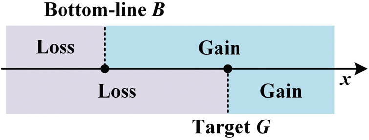
Figure 1: Relationship between reference points and losses and gains
According to the psychological characteristics of loss aversion and Equity Theory, decision-makers are often concerned not with the absolute value of gain or loss but with the relative value. When multiple reference points are observed, the calculation of the gain/loss value is suitable for adopting the mode of processing each reference point separately [29] and then the results are combined. Following this idea, the gain/loss value of attribute xij(tk) relative to the bottom-line reference point Bj(tk) can be expressed as Eq. (2), and its gain/loss value relative to the target reference point Gj(tk) can be expressed as Eq. (3).
y is a gain when y > 0, and y is a loss when y < 0. Based on the separate calculation of the gain/loss value of the two reference points, the gain/loss value based on the two reference points is obtained through the combination as shown in Eq. (4).
where r is the coefficient of the decision mechanism, indicating the relative importance of the decision-makers on the two reference points, 1 > r > 0. When r > 0.5, the decision-maker pays more attention to the bottom-line reference point, while when r < 0.5, the decision-maker pays more attention to the target reference point. When r = 0.5, the decision-maker attaches equal importance to the two reference points while when r = 1, the decision-maker only pays attention to the bottom-line reference point and not the target reference point. When r = 0, it means that the decision-maker focuses only on the target reference point and not the bottom-line reference point.
Fig. 1 and Eq. (4) suggest the following: (1) When the measured value of attribute xi,j(tk) is better than the target reference point Gj(tk),
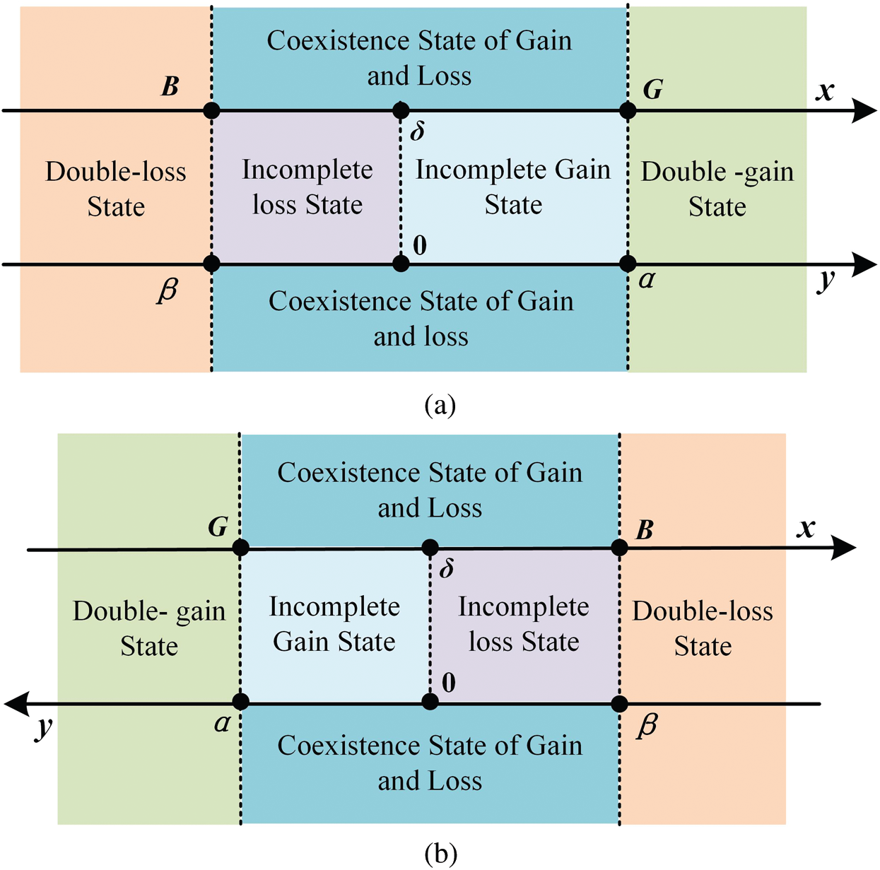
Figure 2: Double reference points and area division. (a) Attribute value is benefit type, (b) attribute value is cost type
3.2 Construction of Attitude Function
Attitude is the essential reflection of decision-makers on the gain/loss [24]. Attitude value is a quantitative description of attitude characteristics. When the attribute value is in the double-gain state, the decision-makers are satisfied. Meanwhile, when the attribute value is in the double-loss state, the decision-maker is dissatisfied. When the attribute value is under the coexistence state of gain and loss, the decision-makers feel hesitant and contradictory. The relationship between gain and loss status and the attitude of decision-makers is shown in Fig. 3.
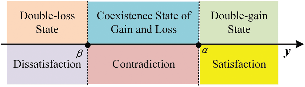
Figure 3: Gain and loss status and attitude
To describe the attitude characteristics quantitatively, numbers greater than 1 are used to express satisfaction; the larger the value, the higher the satisfaction. Meanwhile, numbers less than −1 are used to express dissatisfaction and the smaller the value, the higher the dissatisfaction. The numbers in [−1, 1] indicate contradictory and hesitant attitudes, the closer the value is to 1, the closer to satisfaction, and the closer the value is to −1, the closer to dissatisfaction. If the decision-maker exhibits a risk-neutral attitude to the gain/loss value, then the correspondence between the attitude value v and the gain/loss value y can be simply expressed as Eq. (7) using a linear function.
In reality, decision-makers often respond to gains with a risk-aversion attitude and deal with losses with a risk-seeking attitude [30,31]. Based on this idea, when the gain/loss value y ≥ 0, the attitude function behaves as a monotonically increasing convex function. Meanwhile, when the gain/loss value y < 0, the attitude function is a monotonically increasing concave function. In other words, the attitude function should be an S type function whose inflection point is at the position of y = 0. The correspondence between attitude value v and the gain/loss value y can be expressed by the power function as Eq. (8).
where ϕ is the preference coefficient, 0 < ϕ < 1.
By comparing Eqs. (7) and (8), we can see that if the prefer ence coefficient ϕ discards value constraints, Eq. (8) becomes Eq. (7) when taking the value 1. That is, when ϕ = 1, decision-makers exhibit risk-neutral attitudes towards losses and gains. When the value range of ϕ is expanded from (0, 1) to [0, 1], Eq. (7) will be unified into Eq. (8). The function curve when the constant ϕ takes different values is shown in Fig. 4.
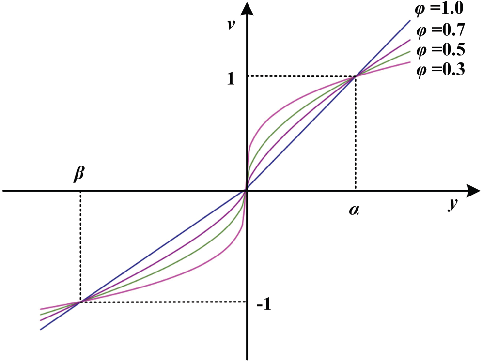
Figure 4: Attitude function
3.3 Construction of Utility Function
In the coexistence state of gain and loss, the more efficient the attitude value, the greater the utility. The utility value increases with the increase of attitude value and decreases with a decrease in attitude value. The utility function u(∙) at this time can be expressed as Eq. (9).
Han [18] and Wang et al. [32] posited that decision-makers will become very sensitive near the bottom-line reference point and a small drop in the attribute value across the bottom-line reference point will cause a “catastrophic” decline in the utility of the decision-makers. Decision-makers extremely circumvent such risks. In other words, when the coexistence state of gain and loss becomes the double-loss state, a qualitative change occurs and the utility value will drop significantly. Supposing
where
From the coexistence state of gain and loss to the double-gain state, it reflects more a change of quantity than a sudden change of quality. Therefore, when the attitude value changes from
where
In summary, the utility function u(∙) can be obtained by combining Eqs. (9)–(11) as shown in Eq. (12). The utility curve obtained from Formula (12) is shown in Fig. 5.
where
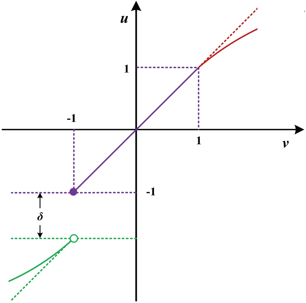
Figure 5: Utility curve
Determining the time weight reasonably is a key issue in the DMADM model. Generally speaking, the value of information will decay over time. At present, most methods for determining the weight of time are based on the principle of “preference of the new to the old.” That is, new information is given greater weight, and old information is given a lower weight. Assuming that the attenuation rate of information is λ(
where tp – tk is the interval of period tk and the current period tp, tp – tk = p − k. When the attenuation rate λ takes different values, the attenuation function curve can be expressed as shown in Fig. 6.
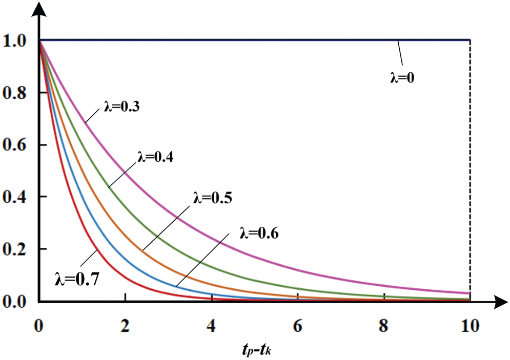
Figure 6: Time attenuation function curve
The time weight can be obtained by normalizing z(tk), as shown in Eq. (14). In particular, when λ = 0, z(tk) ≡ 1,
3.4.2 Calculation of Attribute Weights
The weight of attributes in a dynamic decision model may change with time, in contrast to the static decision model. The objective weighting method is used for weighting to utilize fully the loss information in different periods and improve the scientific of decision-making. Common objective weighting methods include the variation coefficient method, entropy weight method, and mean-variance method. The attribute weight is obtained based on the gain/loss value to reflect the difference in profit and loss information. The value range of the gain/loss value is not suitable for weighting using the variation coefficient method and the entropy weight method. Hence, to reflect the degree of difference between gain/loss values, the mean-variance method can be used for weighting. Because the gain/loss values are related closely to the reference point, the mean square error should be calculated separately according to different reference points. The mean square deviation of the gain/loss value based on the bottom-line reference point is shown in Eq. (15). The mean square deviation of the gain/loss value based on the target reference point is shown in Eq. (16).
where
where,
Finally, the two mean square errors are combined and normalized to obtain attribute weights, as shown in Eq. (17).
3.5 Calculation and Ranking of Comprehensive Utility Value
Following previous calculation results, the comprehensive utility value of the alternative can be expressed as shown in Eq. (18).
The larger the comprehensive utility value ui, the better the alternative ai. Decision-makers will become very sensitive near the bottom-line reference point and a small drop across the bottom-line reference point will cause a huge decline in the utility [18,32]. If the virtual alternative with the attribute value equal to the bottom-line value is called the bottom-line alternative ab, then following the calculation of the utility value and the aggregation method, the comprehensive utility value of the bottom-line alternative is ub = −1. Similarly, if the virtual alternative with the attribute value equal to the target value is called the target alternative ag, then following the calculation of the utility value and the aggregation method, the comprehensive utility value of the target alternative is ug = 1. Regarding the division of decision-makers’ attitudes in Fig. 3, the alternative with comprehensive utility value u > 1 is called the satisfaction alternative, the alternative with comprehensive utility value u < −1 is called the dissatisfaction alternative, and the alternative with integrated utility value u∈[−1, 1] is called hesitation alternative. The relationship between the different types of alternatives and utility values is shown in Fig. 7. The satisfaction alternative is better than the hesitation alternative and the hesitation alternative is better than the dissatisfaction alternative.
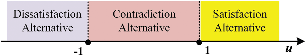
Figure 7: Alternative classification
The steps of the MADM method based on double reference points in a dynamic environment are as follows:
Step 1: Start making decisions.
Step 2: Obtain the decision matrix and double reference points in different periods through a survey.
Step 3: Calculate the gain/loss values according to Eqs. (2)–(4) and obtain the gain/loss matrix for different periods.
Step 4: Calculate the attitude values corresponding to different gain/loss values according to Eq. (8) and obtain the attitude matrix for different periods.
Step 5: Calculate the utility value corresponding to different attitude values according to Eq. (12).
Step 6: Calculate the weight of the period according to Eqs. (13), (14); and according to Eqs. (15)–(17), calculate the attribute weight vector under each period using the mean-variance method.
Step 7: Calculate the comprehensive utility value of alternatives according to Eq. (18), and then classify, rank, and select alternatives.
Step 8: End.
4 Application of Decision-Making Methods in Smart City Evaluation
4.1 Description of Smart City Evaluation Issues
With the rapid development of RFID technology [34,35], internet of things technology [36], network technology [37,38], big data [39] and other technologies, the construction and development of smart cities have been given considerable attention by many governments and organizations [40–42]. The analysis of the development level of smart cities has also attracted the attention of many scholars. For example, Shen et al. [43] used the entropy weight method and Technique for Order of Preference by Similarity to Ideal Solution (TOPSIS) method to evaluate the development level of smart cities in 44 cities of China. Ren et al. [44] built an evaluation index system from five aspects that include smart infrastructure, smart government, and smart people’s livelihood to evaluate the development level of smart cities. Zhang et al. [45] established an evaluation index system based on the needs of residents and used a fuzzy analytic hierarchy process to evaluate the development level of smart cities. In general, most existing studies have used static methods for analysis and evaluation and did not consider the dynamic perspective. The construction of smart cities is a long-term and gradual process. The static evaluation method has obvious shortcomings in describing its intellectualization process and development stage. Moreover, the development stage of urban intelligence should also be measured from the perspective of dynamic evaluation [46].
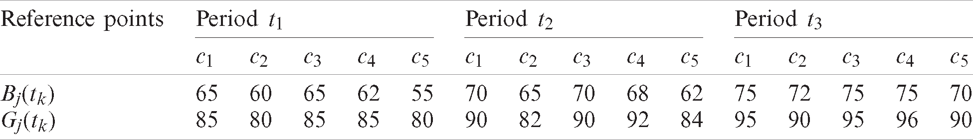
The researchers are ready to evaluate the development level of smart cities of six cities a1, a2, a3, a4, a5, and a6. Considering that the development of smart cities is a dynamic process, the evaluation information covers three periods, that is, t1, t2, and t3. Drawing on [44], five aspects, including smart infrastructure (c1), smart government (c2), smart livelihood (c3), smart production (c4), and innovation drive (c5) are taken as starting points and the evaluation values of each city in each attribute in different periods are obtained using the expert scoring method, as shown in Tab. 1. According to the development background and requirements of the different periods and following the principle of gradually increasing requirements, the bottom-line reference point and target reference point are determined as shown in Tab. 2. Now it is required to evaluate and analyze the development level of smart cities of the six cities according to the above information.
Table 1: Evaluation information
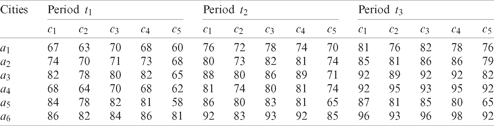
Table 2: Double reference points
4.2 Evaluation of Smart City Development Level
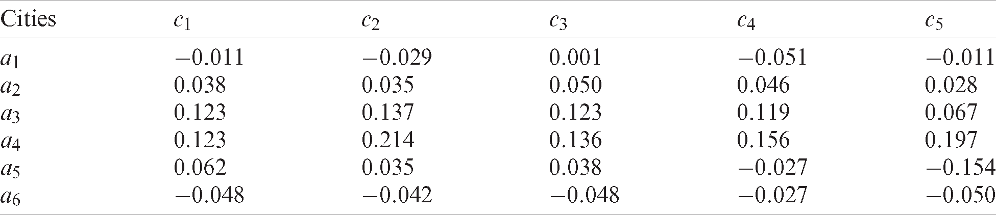
The decision-making method mentioned above is used to evaluate the development level of smart cities. First, following Eqs. (2) and (3), the gain/loss matrix relative to bottom-line reference point B and target reference point G can be obtained. Assuming that the decision-maker pay more attention to the bottom-line reference point than to the target reference point, the decision mechanism coefficient r is taken as 0.6, and the comprehensive gain/loss matrix can be obtained according to Eq. (4), as shown in Tabs. 3–5.
Table 3: Gain/loss matrix for period t1
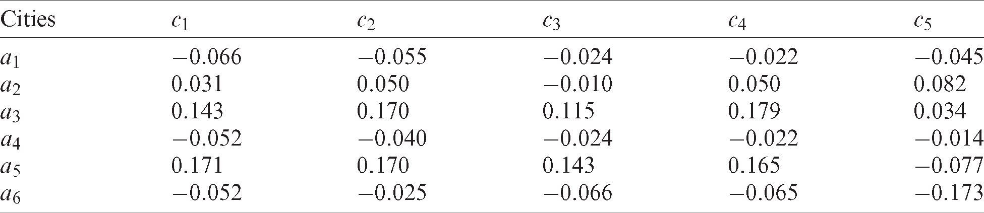
Table 4: Gain/loss matrix for period t2
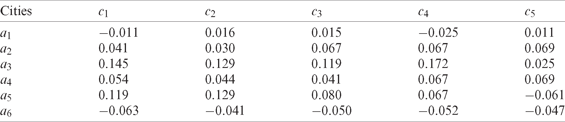
Table 5: Gain/loss matrix for period t3
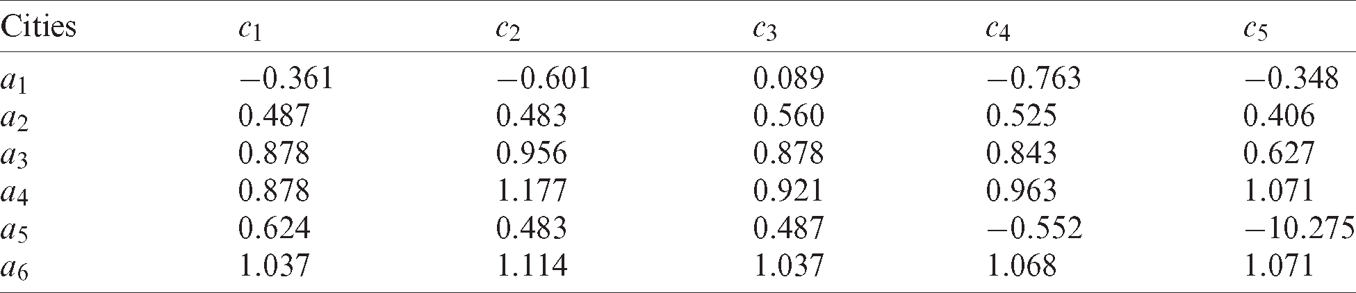
Then, based on the gain/loss matrix, the preference coefficient ϕ is 0.5 according to experience and the attitude matrix can be obtained using Eq. (8). The utility value corresponding to different attitude values are determined according to Eq. (12), where δ is 10 according to the preference of the evaluator. The results are shown in Tabs. 6–8.
Table 6: Utility matrix for period t1
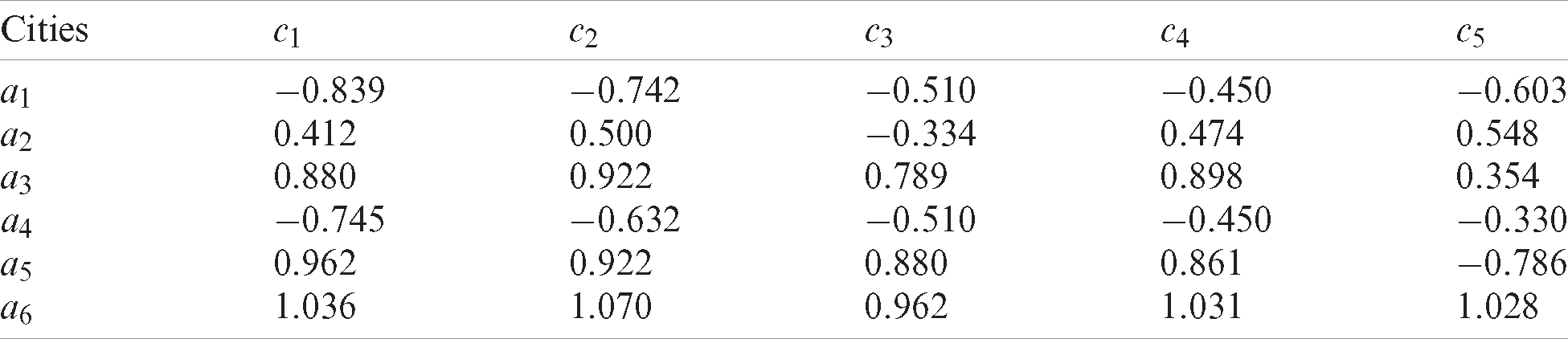
Table 7: Utility matrix for period t2
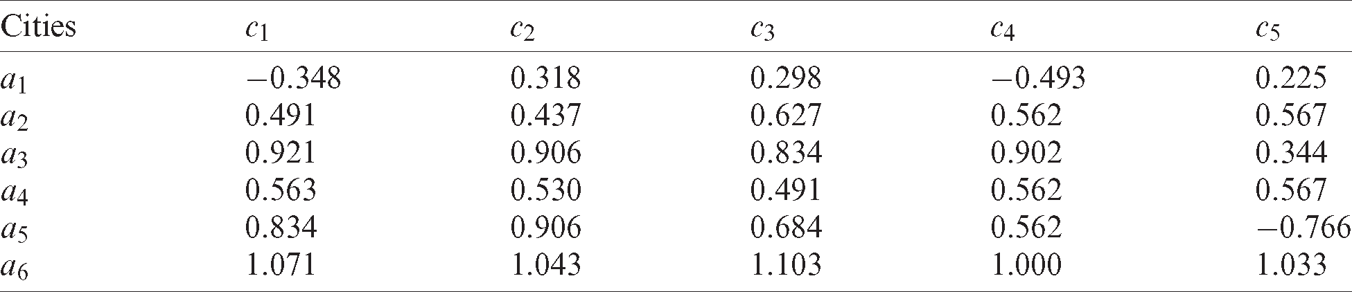
Table 8: Utility matrix for period t3
Then, the attenuation rate λ takes 0.5 and the weight vector
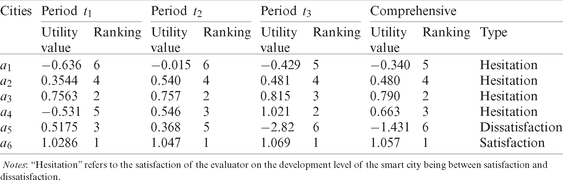
Finally, the comprehensive utility value is obtained by using Eq. (18), and the alternatives are classified and ranked accordingly. The results are shown in Tab. 9. It shows that the smart city development level of city a6 satisfied the evaluators, city a5 dissatisfied the evaluator, and other cities are between satisfaction and dissatisfaction. The specific ranking from good to bad is a6 > a3 > a4 > a2 > a1 > a5.
Table 9: Utility value and ranking
We use the expected utility method, weighted TOPSIS method, and Regret theory to evaluate the development level of smart cities and compare the results with the results of the new decision-making method to further illustrate the difference between the decision-making method proposed in this study and the traditional method. The traditional method is required to provide the time and attribute weights in advance. The weights are calculated using the new decision method to make the results comparable. When using the expected utility method, the weighted arithmetic average operator is used twice to obtain the evaluation result. Meanwhile, when using the weighted TPOSIS method, the closeness of each city in each period is first calculated and the weighted arithmetic average operator is used to fuse the closeness of different periods. When using the Regret theory, the average of bottom-line reference point B and target reference point G is taken as the reference point and then the perception utility of each city in each period is calculated. Then, the weighted arithmetic average operator is used to aggregate the perception utility of different periods. The evaluation results of the development level of smart cities through different methods are shown in Tab. 10.
Table 10: Comparison of different methods
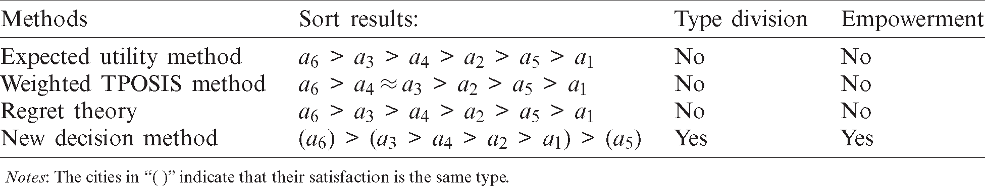
The above comparison shows the following: (1) The results of traditional methods for evaluating the development level of smart cities are basically consistent. (2) The new method can classify the development level of smart cities and determine that the smart city development level of city a6 is in a satisfaction state of decision-makers, city a5 is in a state of dissatisfaction, and other cities are somewhere between satisfaction and dissatisfaction. (3) The ranking result in a new decision-making method for cities with satisfactory and intermediate states (a1, a2, a3, a4, a6) is basically consistent with that of the traditional method. (4) The new method can effectively weigh periods and attributes.
As people face an increasingly complex environment, the use of multi-period decision information for dynamic decision analysis has become a growing trend. The bottom-line and target have important influence on decision-making behavior and they can be used as reference points to describe in more detail the psychological behavior characteristics of the decision-maker. Hence, this paper proposes a DMADM method based on two reference points, namely, bottom-line and target. First, the bottom-line reference point and target reference point are set to reflect the psychological and behavioral characteristics of decision-makers. The two reference points are used to divide the entire range of attribute values into three state intervals of “double gain,” “double loss,” and “coexistence of gain and loss” The state interval “coexistence of gain and loss” can be divided into “incomplete income” and “incomplete loss”. Second, gain/loss function, attitude function, and utility function are established according to the psychological behavior characteristics of decision-makers. The weight of the period is determined using the principle of information attenuation, while the attribute weight was calculated based on the mean square error. Finally, the methods of alternatives classification and ranking are given based on the comprehensive utility value.
The new decision-making method is compared with the expected utility method, weighted TOPSIS method, and Regret theory through the application of examples. The new decision-making method has the following advantages: (1) The new decision-making method can divide the alternatives into three types, namely, satisfaction, hesitation, and dissatisfaction, and it can effectively judge the degree to which the alternatives meet the requirements of the decision-makers. (2) The new decision-making method can effectively solve the weighting problem of periods and attributes. (3) While the new decision-making method screens out unsatisfactory alternatives effectively, the ranking results of other alternatives are consistent with traditional methods.
This study can provide a reference for research on multi-reference MADM and DMADM problems, and further enrich the research connotation of MADM theory and methods. However, this paper only studies the DMADM problem with double reference points and decision information as crisp number. The decision mechanism coefficient r, attenuation rate λ, and other related coefficients in this paper require further discussion. The DMADM problem with more than two reference points and the double reference points DMADM problem with fuzzy number or linguistic variable will be discussed in the future work.
Funding Statement: This work was supported in part by the National Natural Science Foundation of China under Grant 62003379, Natural Science Foundation of Guangdong Province under Grant 2018A030313317, Special Research Project on the Prevention and Control of COVID-19 Epidemic in Colleges and Universities of Guangdong under Grant 2020KZDZX1118, Guangzhou Science and Technology Program under Grant 202002030246, Research Project and Development Plan for Key Areas of Guangdong Province under Grant 2020B0202080002, Guangzhou Key Research Base of Humanities and Social Sciences (Research Center of Agricultural Products Circulation in Guangdong-Hong Kong-Macao Greater Bay Area).
Conflicts of Interest: The authors declare that they have no conflicts of interest to report regarding the present study.
1. X. Z. Zhang, C. X. Zhu and L. Zhu. (2014). “A method of dynamic multi-attribute decision making based on variable weight,” Control and Decision, vol. 29, no.~3, pp. 494–498,~. [Google Scholar]
2. Y. Chen and B. Li. (2011). “Dynamic multi-attribute decision making model based on triangular intuitionistic fuzzy numbers,” Scientia Iranica, vol. 18, no.~2, pp. 268–274,~. [Google Scholar]
3. B. Pablo, R. Eugénio, H. Varum and F. Rodrigues. (2020). “A dynamic multi-criteria decision-making model for the maintenance planning of reinforced concrete structures,” Journal of Building Engineering, vol. 27, no.~5, pp. 100971,~. [Google Scholar]
4. F. Li, F. P. Wu and L. X. Chen. (2020). “Harmonious allocation of carbon emission permits based on dynamic multiattribute decision-making method,” Journal of Cleaner Production, vol. 248, no.~7, pp. 119184,~. [Google Scholar]
5. S. Yao, Z. Jiang, N. Li, H. Zhang and N. Geng. (2011). “A multi-objective dynamic scheduling approach using multiple attribute decision making in semiconductor manufacturing,” International Journal of Production Economics, vol. 130, no.~1, pp. 125–133,~. [Google Scholar]
6. F. Chen, M. Li and H. Wu. (2017). “GACRM: A dynamic multi-Attribute decision making approach to large-Scale web service composition,” Applied Soft Computing, vol. 61, no.~11, pp. 947–958,~. [Google Scholar]
7. Y. Dong, H. Zhang and H. V. Enrique. (2016). “Consensus reaching model in the complex and dynamic MAGDM problem,” Knowledge Based Systems, vol. 106, no.~6, pp. 206–219,~. [Google Scholar]
8. J. Q. Yang, Z. L. Shi, Y. Y. Huang and L. Cheng. (2017). “Developing dynamic intuitionistic normal fuzzy aggregation operators for multi-attribute decision-making with time sequence preference,” Expert Systems with Application, vol. 82, no.~10, pp. 344–356,~. [Google Scholar]
9. X. H. Xu and S. L. Liu. (2020). “Dynamic large group emergency decision-making method considering time series,” Control and Decision, vol. 35, no.~11, pp. 2609–2618,~. [Google Scholar]
10. K. L. Milkman, M. C. Mazza, L. L. Shu, C. J. Tsay and M. H. Bazerman. (2012). “Policy bundling to overcome loss aversion: A method for improving legislative outcomes,” Organizational Behavior and Human Decision Processes, vol. 117, no.~1, pp. 158–167,~. [Google Scholar]
11. L. Luke. (2019). “Adaptive loss aversion and market experience,” Journal of Economic Behavior & Organization, vol. 168, pp. 43–61,~. [Google Scholar]
12. W. Niu and Q. Zeng. (2018). “Corporate financing with loss aversion and disagreement,” Finance Research Letters, vol. 27, no.~11, pp. 80–90,~. [Google Scholar]
13. E. Garbarino, R. Slonim and M. C. Villeval. (2019). “Loss aversion and lying behavior,” Journal of Economic Behavior & Organization, vol. 158, no.~6, pp. 379–393,~. [Google Scholar]
14. F. Pei, L. L. Zhang and A. Yan. (2018). “Algorithm of dynamic hybrid multi-attribute group decision-making based on two reference points,” Control and Decision, vol. 33, no.~3, pp. 571–576,~. [Google Scholar]
15. C. S. Ying, Y. L. Li, K. S. Chin, H. T. Yang and J. Xu. (2018). “A new product development concept selection approach based on cumulative prospect theory and hybrid-information MADM,” Computers & Industrial Engineering, vol. 122, no.~1, pp. 251–261,~. [Google Scholar]
16. H. D. Wang, X. H. Pan, J. Yan, J. L. Yao and S. F. He. (2020). “A projection-based regret theory method for multi-attribute decision making under interval type-2 fuzzy sets environment,” Information Sciences, vol. 512, no.~1, pp. 108–122,~. [Google Scholar]
17. H. Li, J. J. Zhu and S. T. Zhang. (2016). “Risk group decision-making method considering double reference point in cumulative prospect theor,” Operation Research and Management Science, vol. 25, no.~3, pp. 117–124. [Google Scholar]
18. J. Han, X. Y. Teng, S. X. Ye and J. Chai. (2018). “A decision-making method of tri-reference point theory considering robustness of the cooperative network,” Operation Research and Management Science, vol. 27, no.~11, pp. 30–39,~. [Google Scholar]
19. A. D. Roy. (1952). “Safety first and the holding of assets,” Econometrica, vol. 20, no.~3, pp. 431–449,~. [Google Scholar]
20. Z. R. Wang and T. T. He. (2020). “Purchase behavior of structured products based on tri-reference point theory,” Control and Decision, vol. 55, no.~3, pp. 676–685,~. [Google Scholar]
21. J. G. March and Z. Shapira. (1992). “Variable risk preferences and the focus of attention,” Psychological Review, vol. 99, no.~1, pp. 172–183,~. [Google Scholar]
22. S. Highhouse and P. Yuce. (1996). “Perspectives, perceptions, and risk-taking behavior,” Organizational Behavior and Human Decision Processes, vol. 65, no.~2, pp. 159–167,~. [Google Scholar]
23. X. F. Xie and X. T. Wang. (2003). “Risk perception and risky choice: Situational, informational and dispositional effects,” Asian Journal of Social Psychology, vol. 6, no.~2, pp. 117–132,~. [Google Scholar]
24. H. Huang, K. Cai and K. Fang. (2019). “A method of multi-attribute decision making with double-reference points and its application in location of agricultural products logistics center,” IEEE Access, vol. 7, no.~1, pp. 167629–167638,~. [Google Scholar]
25. J. Wang, X. Jin, Y. Yuan and X. Wang. (2015). “Loss aversion portfolio optimal model with dynamic reference point,” Operation Research and Management Science, vol. 6, pp. 51–57,~. [Google Scholar]
26. X. Y. Li, X. M. Li and X. W. Li. (2016). “Dynamic reference points based bounded rational multi-agent model of route choice,” Complex Systems and Complexity Science, vol. 13, no.~2, pp. 27–35,~. [Google Scholar]
27. L. Wang, Z. X. Zhang and Y. M. Wang. (2015). “A prospect theory-based interval dynamic reference point method for emergency decision making,” Expert Systems with Application, vol. 42, no.~23, pp. 9379–9388,~. [Google Scholar]
28. H. Jiang and X. Ren. (2019). “Model of passenger behavior choice under flight delay based on dynamic reference point,” Journal of Air Transport Management, vol. 75, no.~4, pp. 51–60,~. [Google Scholar]
29. L. D. Ordónez, T. Connolly and R. Coughlan. (2000). “Multiple referencepoints in satisfaction and fairness assessment,” Journal of Behavioral Decision Making, vol. 13, no.~3, pp. 329–344,~. [Google Scholar]
30. X. Luo, W. M. Li and X. Z. Wang. (2019). “Decision method for two-sided matching based on double reference points,” Control and Decision, vol. 34, no.~6, pp. 1286–1292,~. [Google Scholar]
31. D. Kahneman and A. Tversky. (1979). “Prospect theory: An analysis of decision under risk,” Econometrica, vol. 47, no.~2, pp. 263–291,~. [Google Scholar]
32. X. T. Wang and J. G. Johnson. (2012). “A tri-reference point theory of decision making under risk,” Journal of Experimental Psychology General, vol. 141, no.~4, pp. 743–756,~. [Google Scholar]
33. G. B. He and Y. J. Yu. (2006). “Reference point effect in the decision making process,” Advances in Psychological Science, vol. 14, no.~3, pp. 408–412,~. [Google Scholar]
34. J. Su, Z. Sheng, A. X. Liu and Y. Chen. (2020). “A partitioning approach to RFID identification,” IEEE/ACM Transactions on Networking, vol. 28, no.~5, pp. 2160–2173,~. [Google Scholar]
35. J. Su, Z. Sheng, A. X. Liu, Y. Han and Y. Chen. (2020). “Capture-aware identification of mobile RFID tags with unreliable channels,” IEEE Transactions on Mobile Computing, . Early Access, https://doi.org/10.1109/TMC.2020.3024076. [Google Scholar]
36. X. Zhao, H. Zhu, X. Qian and C. Ge. (2019). “Design of intelligent drunk driving detection system based on Internet of Things,” Journal of Internet of Things, vol. 1, no.~2, pp. 55–62,~. [Google Scholar]
37. J. Su, R. Xu, S. Yu, B. Wang and J. Wang. (2020). “Idle slots skipped mechanism based tag identification algorithm with enhanced collision detection,” KSII Transactions on Internet and Information Systems, vol. 14, no.~5, pp. 2294–2309,~. [Google Scholar]
38. J. Su, R. Xu, S. Yu, B. Wang and J. Wang. (2020). “Redundant rule detection for software-defined networking,” KSII Transactions on Internet and Information Systems, vol. 14, no.~6, pp. 2735–2751,~. [Google Scholar]
39. Y. L. Bi, Y. X. Ouyang, G. Sun, P. Guo, J. J. Zhang et al. (2020). , “Big data audit of banks based on fuzzy set theory to evaluate risk level,” Journal on Big Data, vol. 2, no.~1, pp. 9–18,~. [Google Scholar]
40. A. H. Alavi, J. Pengcheng, W. G. Buttlar and L. Nizar. (2018). “Internet of things-enabled smart cities: State-of-the-art and future trends,” Measurement, vol. 129, no.~6, pp. 589–606,~. [Google Scholar]
41. S. Jha, L. Nkenyereye, G. P. Joshi and E. Yang. (2020). “Mitigating and monitoring smart city using internet of things,” Computers, Materials & Continua, vol. 65, no.~2, pp. 1059–1079,~. [Google Scholar]
42. N. Khelifi, K. Benahmed and F. Bounaama. (2020). “A cryptographic-based approach for electricity theft detection in smart grid,” Computers, Materials & Continua, vol. 63, no.~1, pp. 97–117,~. [Google Scholar]
43. L. Y. Shen, Z. H. Huang and S. W. Wong. (2018). “A holistic evaluation of smart city performance in the context of China,” Journal of Cleaner Production, vol. 200, no.~4, pp. 667–679,~. [Google Scholar]
44. L. Ren, H. T. Zhang and M. Z. Wei. (2019). “Research on the evaluation of development level of smart city based on entropy TOPSIS model,” Information Studies: Theory & Application, vol. 42, no.~7, pp. 113–118. [Google Scholar]
45. Y. J. Zhang, F. Y. Liu, Z. Q. Gu, Z. X. Chen and A. H. Li. (2019). “Research on smart city evaluation based on hierarchy of needs,” Procedia Computer Science, vol. 162, no.~3, pp. 467–474. [Google Scholar]
46. S. L. Luo and H. X. Xia. (2018). “Thinking on assessment of smart cities from the aspect of capability maturity,” Science Research Management, vol. 39, no.~S1, pp. 284–289. [Google Scholar]
 | This work is licensed under a Creative Commons Attribution 4.0 International License, which permits unrestricted use, distribution, and reproduction in any medium, provided the original work is properly cited. |