Computers, Materials & Continua DOI:10.32604/cmc.2021.016307
Article

Computer Decision Support System for Skin Cancer Localization and Classification

Muhammad Attique Khan1, Tallha Akram2, Muhammad Sharif1, Seifedine Kadry3 and Yunyoung Nam4,*

1Department of Computer Science, COMSATS University Islamabad, Wah Campus, 47040, Pakistan
2Department of Computer and Electrical Engineering, COMSATS University Islamabad, Wah Campus, 47040, Pakistan
3Department of Mathematics, Beirut Arab University, Beirut, Lebanon
4Department of Computer Science and Engineering, Soonchunhyang University, Asan, Korea
*Corresponding Author: Yunyoung Nam. Email: ynam@sch.ac.kr
Received: 30 December 2020; Accepted: 02 February 2021

Abstract: In this work, we propose a new, fully automated system for multiclass skin lesion localization and classification using deep learning. The main challenge is to address the problem of imbalanced data classes, found in HAM10000, ISBI2018, and ISBI2019 datasets. Initially, we consider a pre-trained deep neural network model, DarkeNet19, and fine-tune the parameters of third convolutional layer to generate the image gradients. All the visualized images are fused using a High-Frequency approach along with Multilayered Feed-Forward Neural Network (HFaFFNN). The resultant image is further enhanced by employing a log-opening based activation function to generate a localized binary image. Later, two pre-trained deep models, Darknet-53 and NasNet-mobile, are employed and fine-tuned according to the selected datasets. The concept of transfer learning is later explored to train both models, where the input feed is the generated localized lesion images. In the subsequent step, the extracted features are fused using parallel max entropy correlation (PMEC) technique. To avoid the problem of overfitting and to select the most discriminant feature information, we implement a hybrid optimization algorithm called entropy-kurtosis controlled whale optimization (EKWO) algorithm. The selected features are finally passed to the softmax classifier for the final classification. Three datasets are used for the experimental process, such as HAM10000, ISBI2018, and ISBI2019 to achieve an accuracy of 95.8%, 97.1%, and 85.35%, respectively.

Keywords: Skin cancer; convolutional neural network; lesion localization; transfer learning; features fusion; features optimization

1  Introduction

Skin cancer, as per stats from the World Health Organization (WHO) [1], is one of the most deadly types of cancer worldwide [2,3]. According to the reports, the number of deaths in the next two years will be doubled. However, the death rate could be controlled if the infection is diagnosed in the earlier early stages [4]. Skin cancer typically has seven major types, but the most common types are basal cell carcinoma, squamous cell carcinoma, and malignant melanoma. Melanoma is the most deadly skin cancer and causes several deaths worldwide [5]. According to WHO, in 2020 only, the number of melanoma cases is increased, but the total number of deaths is decreased with a ratio of 5.3%. The estimated number of melanoma cases in the USA alone, since 2020, will be 196,060. From the numbers around 95,710 will be noninvasive, and 100,350 will be invasive (Skin Cancer Facts & Statistics, 2020). However, based on the previous reports, the number of new invasive cases has increased by 47% in the last ten years. Timely identification of skin cancer increases the survival rate by 95% [6]. This cancer is primarily diagnosed using clinical methods such as ABCDE rules, a 3-point checklist, and a 7-point checklist. However, these methods face a lot of constraints including unavailability of experts, limited resources, time deficiency, etc. [7,8].

Dermoscopy is a new imaging technology used for skin lesion diagnosis with the drawbacks of its high cost, limited number of expert dermatologists and the diagnosis time [9,10]. The skin lesions are irregular in shape and texture, which is another factor for an inaccurate identification [11]. Researchers actively working in the domain of computer vision and machine learning introduced several computer-aided diagnosis (CAD) techniques to identify skin cancer [12]. A CAD system can be helpful for dermatologists as a second opinion [13]. The classical techniques are introduced between 2010–2016 and before 2010 [14]. These conventional techniques mostly were based on thresholding and clustering [15]. Moreover, machine learning techniques are used for the binary classification purposes and on the balanced data. The main theme of these techniques is to extract the handcrafted features including shape, color, point, and texture, and later use them for the classification purpose [16].

Recently, deep learning algorithms are utilized to develop computerized medical image analysis algorithms [17,18]. Using deep learning, researchers achieved remarkable results, especially stomach and skin cancer lesions classification [19,20]. The results of deep learning techniques are much improved compared to the conventional techniques [21,22]. Moreover, the information fusion of deep learning model also showed improved performance in medical diseases diagnosis [23,24]. Recently, Huang et al. [25] presented a lightweight deep learning approach for skin lesion classification. They employed two pre-trained models named EfficientNet and Densenet and optimize their features for multiclass classification. This work was tested on the HAM10000 dataset and achieved an accuracy of 85.8%. The main advantage of this work is that it is applicable in mobiles for skin lesion diagnosis. Carcagnì et al. [26] presented a convolutional neural network (CNN) approach for multiclass skin cancer classification. They initially implemented Densenet deep model and fine-tuned it according to the dataset classes. Later they extracted the more relevant features and classified them using SVM. The experimental process was conducted on the Ham10000 dataset and achieved an accuracy of 90%. This method is only useful for balanced class datasets.

Thurnhofer-Hemsi et al. [27] presented an ensemble of a deep learning model for multiclass skin cancer classification. They employed five pre-trained deep models such as Googlenet, Inception3, Densenet201, Inception-ResNetV2, and MobileNetV2. They performed fine-tuning and train using transfer learning. After that, they performed a plain classifier and hierarchy of classifiers approach for final classification. For the experimental process, the HAM10000 dataset was used and achieved an accuracy of 87.7%. They conclude that the Densenet model is performed well, and overall, this work is useful for the balanced dataset. Mohamed et al. [28] introduced a deep CNN-based approach for multiclass skin cancer classification. They implemented this method in two factors. First, they train the model on all deeply connected layers. In the second, they balance the data to resolve the issue of data imbalancing. After that, they selected two pre-trained models named Densenet121 and Mobilenet for the classification purpose. The fine-tuned these models and map features for the classification phase. A HAM10000 dataset is used for the experimental process and achieved an accuracy of 92.7%. Because of the balanced training data, this model is useful for Mobile applications. Chaturvedi et al. [29] presented a deep CNN-based computerized approach for multiclass skin cancer classification. They initially normalize images and resized according to the deep models. Later, five pre-trained models are selected and fine-tuned. Deep features are extracted from each model and performed classification. The classification performance is evaluated on balanced dataset HAM10000 and achieved an accuracy of 92.83%. The main concept in this work was the fusion of different neural network information for better classification performance. Shahin et al. [30] ensembles two deep learning network features for the classification of skin cancer. They used ResNet50 and InceptionV3 models for this work. The experimental process was performed on HAM10000 and ISBI2018 datasets and achieved 89.9% and 89.05% accuracy. Almaraz-Damian et al. [31] introduced a fusion framework for skin cancer classification from dermoscopic images. They fused handcrafted features and clinical features such as ABCDE to better lesion information at the first stage. In the next phase, deep CNN features are also extracted and fused with first phase features. The classification is performed by L.R., SVM, and relevant vector machine (RVM). For the experimental process, they used the ISBI2018 dataset and achieved an accuracy of 92.4%. Moreover, authors in [32] presented a residual deep learning framework and achieved an accuracy of above 93% using ISBI2018 dataset.

The rest of the manuscript is organized as follows: Problem statement and major novelties are presented in Section 2. Proposed CAD system is described in the Section 3. Section 4 represents the experimental results and analysis. Finally conclusion is given in Section 5.

2  Problem Statement and Novelties

According to research by [33] poor lesion segmentation extract poor features, which later degrades the classification accuracy. The poor contrast skin lesions are the main factor for poor segmentation; therefore, it is essential to improve local contrast before the lesion segmentation step. The second problem which is facing in the studies mentioned above is imbalanced datasets. The researchers resolve this issue by employing data augmentation, and few of them balance the datasets based on a minimum class count. But this is not a good approach because several images are ignored in the training process. Multiclass skin cancer is not an easy process due to the high similarity among skin lesions shown in Fig. 1. In this figure, it is demonstrated that bcc and bkl lesions have high similarity. Similarly, melanoma and vasc lesion have high similarity. To handle this issue, more relevant and strong features are required. Several extracted features are irrelevant, and few of them are redundant; hence, it is essential to remove those features before the classification phase.

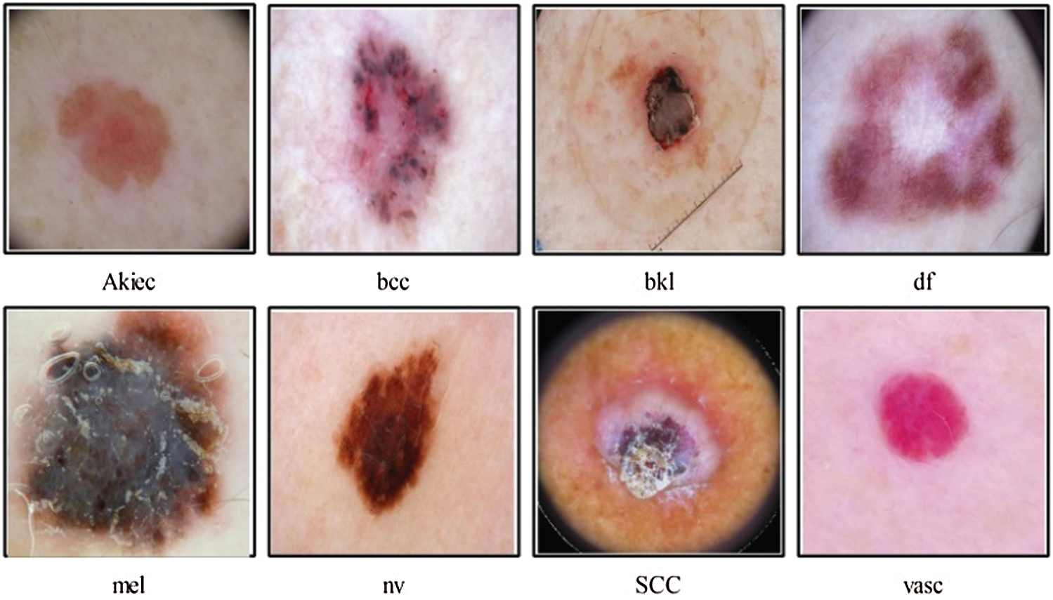
Figure 1: Sample skin lesion types of HAM10000 dataset [34]

In this work, our major contributions are as follows:

     i)  We consider a pre-trained deep CNN model named Darknet19 to apply fine tuning for optimal weights generation. A third convolutional layer is utilized to fetch the gradient information after the visualization. Later, all 128 visualized images are fused using the novel High-Frequency along with feed-forward neural network (HFaFFNN). The fused image is further enhanced by employing a log-opening based activation function.

    ii)  Two pre-trained deep neural networks, Drarknet53 and NasNetMobile (NMobileNet), are fine-tuned and trained through transfer learning. The features from the second last layers of both models are extracted and fused using a new approach, named Parallel max-entropy correlation (PEnC).

   iii)  A feature selection criteria is also proposed using biologically inspired whale feature optimization (WFO) algorithm controlled using entropy and kurtosis based activation functions. Through this function, the best features are selected for final classification.

3  Proposed Methodology

A new end to end computerized method is proposed in this work for multiclass skin lesion localization and classification. Two main phases are included in this method. In the first phase, skin lesions are localized using a new CNN and image fusion-based approach. In the second phase, two pre-trained models are fine-tuned and trained using transfer learning. Features are extracted from the last feature layers and performed fusion using a new approach named Parallel Entropy Correlation (PEnC). After the fusion process, a new hybrid optimization method is implemented, named Entropy Kurtosis controlled Whale Optimizer (EKcWO), for the optimal features selection. The selected features are classified using Softmax classifier for final prediction accuracy. A complete flow diagram of the proposed method is showing in Fig. 2.

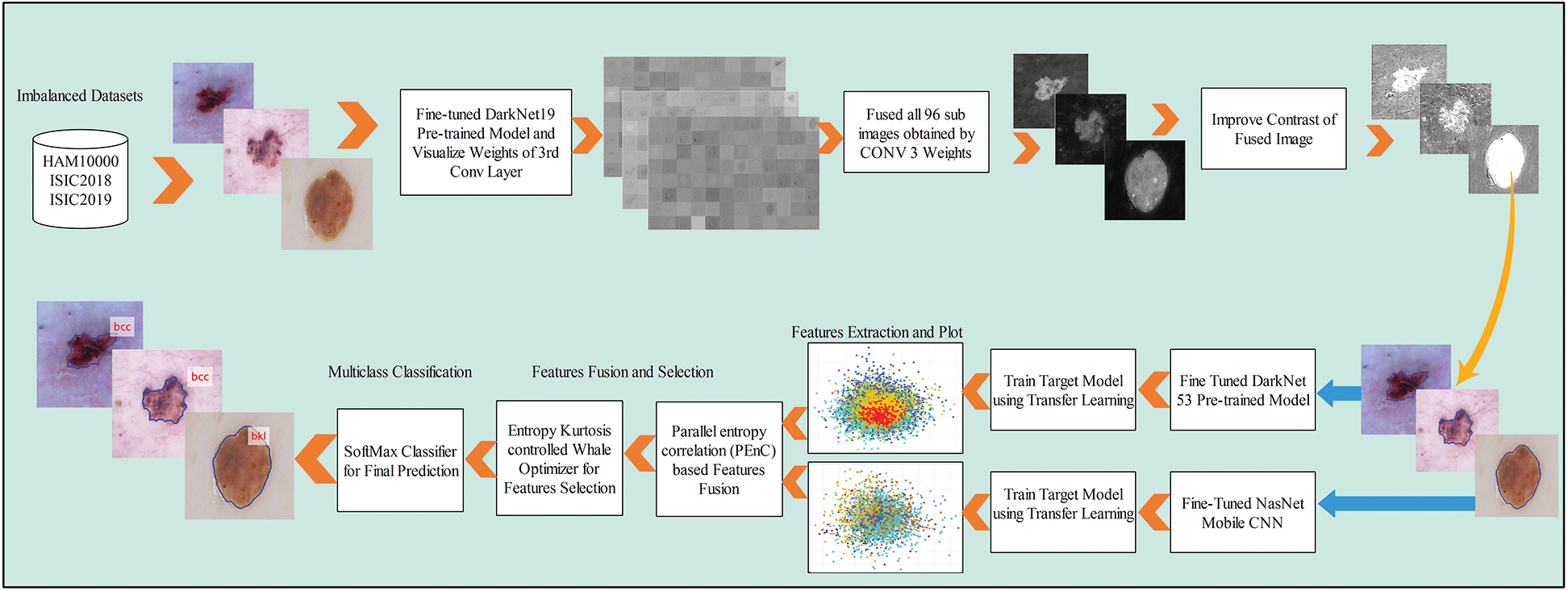
Figure 2: Proposed flow diagram of multiclass skin cancer classification

3.1 Datasets

Three publically available datasets are used in this work for the experimental process. The selected datasets are HAM10000, ISBI2018, and ISBI2019. These datasets are used for the classification tasks. HAM10000 is one of the complex skin cancer datasets containing 10,015 image samples of different resolutions. These images are categorized into seven different lesion classes; akiec, bcc, bkl, df, nv, mel, and vasc. Against each label, the number of images is 327, 541, 1099, 155, 6705, 1113, and 142, respectively. ISBI2018 dataset consists of 10,015 images of seven skin lesion types such as Nevus, Dermatofibroma, Melanoma, Pigmented Bowen’s, Keratosis, Basal Cell Carcinoma, and Vascular. For testing and validation, 1,512 and 193 images are provided without ground truths. The ISIC 2019 skin cancer dataset consists of eight classes: akiec, bcc, df, bkl, mel, SCC, vasc, and nv. This dataset is the combination of HAM10000 and BCN dataset. Moreover, a few clinical images are also added in this dataset. The images in each mentioned class, such as akieck are 867, bcc are 3,323, df is 239, bkl are 2,624, mel is 4,522, nv is 12,875, SCC is 628, and vasc are 253, respectively. A few sample images are also shown in Fig. 1. Based on the above detail, it is show that these datasets are extremely imbalnced. We used testing and validation images jus for labeling. At the same time, the 50:50 approach is considered for training and testing.

3.2 Fine-Tuned DarkNet Model

The arrival of deep learning technology in machine learning has reformed the performance of AI. A deep model consists of a large number of layers. A deep model’s structure starts from the input layer and later processed in the convolutional layer. In this layer, a convolutional operator is used to extract the features called weights. This operation is works based on filters such as filter size and stride. Mathematically, it is formulated as follows: Consider, F0 is an input image of CNN having r rows, c columns, and K color components, where K = 3 in this work. Hence, F0(x,y,z) image is transformed in this model where, 0≤x≤r, 0≤y≤c, and 0≤z≤K are the spatial coordinated. Using these points, a convolutional layer is defined as follows:

Fmap(u,v)=β+∑i=tt∑j=1t∑k=0K-1ωi,j,kF0(u+i,v+j,k)(1)

where feature map of the convolutional layer is represented by Fmap, β represent an offset, and ωi,j,k∈ω×ω×K represent filters of a 2D array. Usually, in a CNN model, many filters are employed to increase the sharpness of object edges. Next, a batch normalization layer is followed to reduces the number of epochs for fast training. Later, a leaky relu (LR) is added to convert the negative values into zero. This function only allows the positive weights for the next step. Mathematically, we defined LR as follows:

LR(f)={0.02fforf<0fforf≥0, wheref∈Fmap(u,v)(2)

Then, a max-pooling layer is applied to reduce the neighborhood. This layer is based on the filter size, and mostly it is defined W×H. In this work, we consider the DarkNet19 pre-trained deep neural network [35] and fine-tuned according to the requirement. Our purpose is the only visualization of convolutional layer features instead of training a model. Therefore, we ignore the last layers and only consider the network to the third convolutional layer, as shown in Fig. 3. The input of this network is 256×256×3. For the first convolutional layer, the filter size is 3×3, the number of filters is 32, the number of channels is 3, and stride 1×1. Following these operations, the learnable weights and bias matrix are of size 3×3×3×32 and 1×1×32. The activation of this matrix of this layer is 256×256×32. Then, batch normalization and leaky relu layers are followed to this convolutional layer. A pooling layer is applied to filter size 2×2 and stride 2.

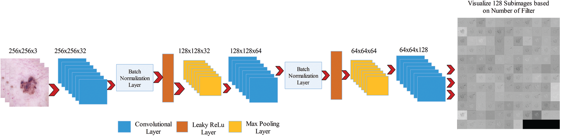
Figure 3: Visualization of fine-tuned convolutional layer weights

After this operation, the activations is 128×128×32. In the next step, a second convolutional laye is added and peformed a convolutional filter of size 3×3, where the number of filters and channels are 64 and 32, respectively. The stride of this layer is 2, and the resultant activation is 128×128×64. The learnable weights and bias matrix are 3×3×32×64 and 1×1×64, respectively. Similar to the first convolutional layer, this follows the batch normalization and leaky relu layers. Then, a pooling layer is added of filter size 2×2 and stride 2. The activations of this layer is 64×64×64.

A convolutional layer is applied to these activations of filter size 3×3, where the number of filters and channels are 128 and 64. For this layer, the activations are 64×64×128, and learnable weights and bias matrix are 3×3×64×128 and 1×1×128, respectively. On in this layer, it is described that a total 128 filters are employed, and for each filter, the matrix size is 3×3×64. Hence, we visualize these filter matrix based on filter size. Visually, it is shown in Fig. 3. In this figure, it is illustrated that a total 128 subimages are reshaped. These images provide the information of input images according to their gradients and pixel-level information, etc.

We consider these 128 images and fused them in one image for better visualization of the lesion part. For this purpose, we implemented a hybrid approach name High-Frequency along with Feed Forward Neural Network (HFaFFNN). In this approach, these images are considered high-frequency images and learn their pixels based on the feed-forward neural network (FwNN), where the FwNN is multilayered. Since a MLFwNN consider a one image pixel as one neuron. The two hidden layers denoted by H are included in this network. The inputs of each layer H are represented by I1̃, I2̃ and total neurons are Ĩ and J̃, respectively. The sigmoid is applied as an activation function of H layers, and linear function is used as an activation function for the output layer, where the output layer is denoted by O^. The output of lth and pth hidden layer is formulated as follows:

Yl(H1)=1[1+e(∑i=1n(ωlixi-βl))],l=1,2,…,J̃ (3)

Yp(H2)=1[1+e(∑l=1J̃(ωplyl-βp))],p=1,2,…,Ĩ (4)

Here hidden layers weights are represented by ωli and ωpl. The outputs of each hidden layer are represented by Yl(H1) and Yp(H2). The base of each hidden layer is represented by βl and βp, respectively. In the last, the output is computed by the following mathematical formulation.

O^n=∑p=1Ĩ(ωnpYp),n=1,2,…,H(5)

To assess this neural network’s training performance, the mean square error rate (MSER) is computed. Based on the MSER value, the weights and bias are updated in the next step. Mathematically, the MSER of this network is calculated as follows:

MSER=1n∑i=1n(O^i-ti)2(6)

Here, O^i is system output image and ti is an target output. This output is judge through the fitness function, which is formulated as follows:

Fit(Xi)= min(1n(O^i-ti)2)(7)

However, in our work, we required a more useful and informative image; therefore, we update the weights and bias of the first hidden layer based on the number of iterations. Here, the number of iterations is the number of image pixel values. Hence, the updated weights and bias are defined as follows:

ξωli=φ(Y^l-xi) (8)

ξβl=φ(Y^l-xi) (9)

Here, updated weights are represented by ξωli and updated bias is represented by ξβl. The learning rate in these equations is defined by φ and the value of φ=0.001. Hence, the newly updated equations are:

βnew=βold+ξβl (10)

ωnew=ωold+ξω (11)

In the last, by employing these updated weights and bias, the fusion is performed. The fusion process is formulated through the following activation function:

hFL,d(x,y)={hIL,d(x,y),forIter(I)≥Iter(B).hJL,d,Otherwsie(12)

Here, hIL,d(x,y) represents high-level decomposition images, L represents levels, d represents directions, and Iter(.) represents the number of iterations per image based on the image pixels, performed by a neural network. Finally, the high-level decomposition pixels are reconstructed by MATLAB image reconstruction function and obtained an output image, shown in Fig. 4 (Fused using the proposed approach). After this step, we applied a hybrid contrast stretching method to increase the pixel’s intensity range (can be seen in Fig. 4 (Contrast stretching)). The logarithmic function is applied for the contrast enhancement, which later converted into a binary form using the Otsu thresholding approach (can be seen in Fig. 4 (binary image)). The active contour-based boundary is drawn on the original image based on the binary lesion image. The localized lesions are used for the text classification task. A few sample qualitative results are illustrated in Fig. 5.

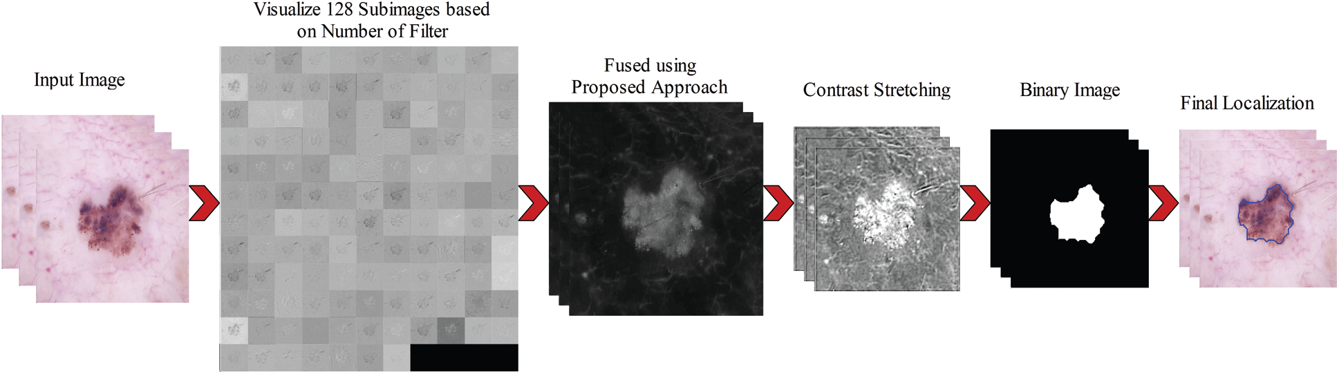
Figure 4: Complete steps involves in the lesion localization using proposed approach

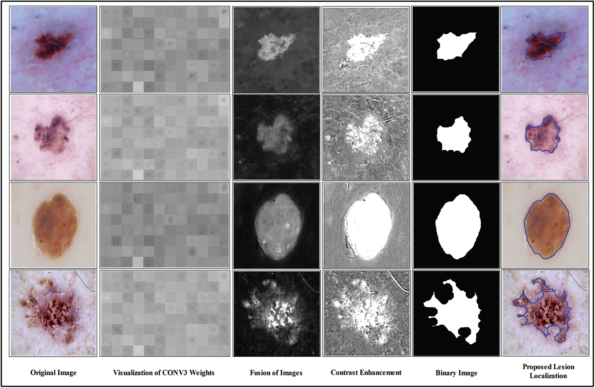
Figure 5: Proposed lesion localization visual results

3.3 Lesion Classification

Transfer Learning: Transfer Learning is reusing a pre-trained deep learning model for a new task [36]. In this task, we used the TL to reuse a pre-trained model (trained on ImageNet 1000 classes) for skin cancer classification (small dataset, max 8 classes). Suppose the source data is Δs representing ImageNet dataset, source labels representing ΔL (1000 object classes), and objective function is representing by Δo. This process can be written as:

Δ={Δs,ΔL,Δo}(13)

Hence, we have three targets as target data representing by ΔT (HAM10000, ISBI2018, and ISBI2019), target labels representing by TL, and objective function TL. It can be defined as:

Δ̃={ΔT,TL,To}(14)

Hence, the transfer learning is applied to Δ̃ by using the knowledge of Δ. Visually, this process is showing in Fig. 6 and mathematically defined as follows:

δ̃=To(ΔT,TL,Δ),=To(ΔT,TL∣Δs,ΔL,Δo)(15)

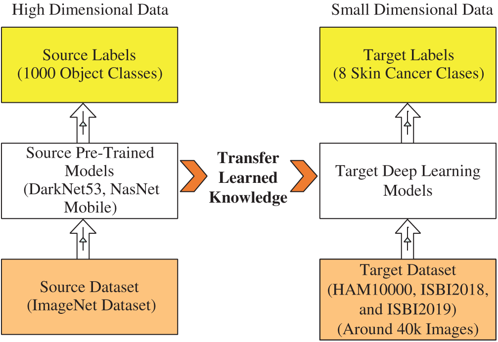
Figure 6: Visual process of transfer learning for feature extraction

Fine Tuned NasNet Mobile CNN: NasNet Mobile [37] is a new CNN architecture constructed by the search architecture of neural network (NN). This architecture contains building blocks, and each block consists of several layers (i.e., convolutional layer, pooling layer, batch normalization layer). These blocks are optimized using reinforcement learning. This process is repeated several times and based on the capacity of a network. A total of 12 blocks are added in this network, where the number of parameters and MACs are 5.3 and 564 M, respectively. This network accepts an input image of h×w×3, where h = 224 and w = 224. These input image pixels are considered as initial weights and passed in the first convolutional layer. In the first convolutional layer, a convolutional operator is applied to filter size 3×3 and stride 2. Moreover, the number of channels and filters for the first layer are 3 and 32, respectively. For most of the blocks, a batch normalization layer is added of value e = 1.0000e −03. This process is continued for all blocks in the network. In the end, all blocks are concatenated and added a few additional layers. Later, a global average pooling layer is added, which followed the last fully connected layer.

We remove the last fully connected layer and add a new layer according to the skin classes’ number in this work. Then, we train the new fine-tuned model using transfer learning. We utilized 50% skin images for training a model due to an imbalanced dataset in the learning process. For training, we initialized a learning rate of 0.002 and a mini-batch size of 64. Moreover, the dropout factor was 0.5, and the weight decay value of 4e −5. After learning this new model, we extract features from the last layer named Global Average Pooling layer (GAP). On this layer, the number of extracted features is 1056, and a vector length is N×1056, where N denotes the number of training images. Mathematically, this vector is represented by λkN, where k denotes feature-length and N denotes sample images.

Fine Tuned DarkNet53 CNN: Darknet53 [38] is the Convolutional Neural Network (CNN) based model, which is used to extract the deep features for object detection and classification [39]. It has 53 layers of deep structure. This model combines the basic feature extraction model of YOLOv2 Darknet19 and the deep Residual Network [40]. This network utilized the 1×1 consecutively and 3×3 convolution layers and residuals. Its smallest component consists of convolution, Batch Normalization (BN), and LeakyRelu layers. The input of this network is h×w×3, where h = 256 and w = 256. The filter size of first convolutional layer is 3×3 and stride 2. The batch normalization layer is followed by the convolutional layer, where the value of epsilon e = 1.000000000000000e −05. In this network, leaku relu is added instead of ReLu layer. Thrugh this layer, convolved weights are converted into positive (0.01) if negative. This process is continued for all 52 convolutional layers. Besides, an additional layer was added which follows the Global Average Pool (GAP) layer and FC layer.

We removed the last fully connected layer and added a new layer according to the number of skin cancer classes. Transfer learning is employed for training this new fine-tuned model. In the learning process, we utilized 50% skin images for training a model due to an imbalanced dataset and the rest 50% for testing. For training, we initialized a learning rate of 0.002 and a mini-batch size of 64. Moreover, the dropout factor was 0.5, and the weight decay value of 4e-5. This new model’s features are extracted from the last layer named Global Average Pooling layer (GAP). On this layer, the number of extracted features is 1056, and a vector length is N×1056, where N denotes the number of training images. Mathematically, this vector is represented by λlN, where l denotes feature-length and N denotes sample images.

3.3.1 Features Fusion

In this article, we proposed a fusion technique using parallel process. The main reason behind the choice of parallel approach instead of serial approach is to get only most relevant features and try to minimize the dimension of feature vector. Consider, we have two deep learning extracted feature vectors, represented by λkN of dimension N×1056 and λlN of dimension N×1056, respectively. Suppose, λfN is a fused feature vector of dimension N× max(length). Initially, we calculated the maximum length feature vectors from the extracted vectors as follows:

Lngi2=length(λkN,λlN),i=1,2. (16)

MLng=max(Lngi2) (17)

Based on MLng, we define a resultant feature vector matrix as: λfN=[λf11,λf22,…,λfN]. Then two entropy values are computed for each vector λrN and λlN as:

H(λkN)=-∑k=1NP(λk) logbP(λk) (18)

H(λlN)=-∑l=1NP(λl) logbP(λl) (19)

Each corresponding vector features are multiplied by their entropy value. The purpose of this operation is to get positive features only. Mathematically, this operation is formulated as follows:

Ψ(λkN)=|λkiN×H(λkN)| (20)

Ψ(λlN)=|λljN×H(λlN)| (21)

Here, Ψ(λkN) and Ψ(λlN) are two updated feature vectors and each value in both vectors are positive. A Pearson Correlation Coefficient (PCC) is applied and fused features based on the positive correlation value. As mentioned at the start of the fusion process that our fused vector length of dimension N×1056; hence, this process is continued as per the length of a fused vector. Mathematically, the PCC formulation is defined as follows:

r̃=∑ (λki-λkN¯)(λlj-λlN¯)∑ (λki-λkN¯)2∑ (λlj-λlN¯)2(22)

Here, PCC is represented by r̃, λki represents an ith feature of vector Ψ(λkN), λlj represents a jth feature of vector Ψ(λlN). Similarly, the mean value of each vector is represented by λkN¯ and λlN¯, respectively. Through r̃, we get the strength between the ith and jth features as follows:

Vectors={λfN,forr̃(Ψ(λkN)i,Ψ(λlN)j)≥0.4λnfNforOtherwise(23)

where, λfN is a fused vector. The features in this vector are higher correlated of value greater than 0.4, selected in a fused vector and λnfN vector features are ignored. As mentioned above that this process is continued till the vector is completed. If fused vector length is not completed in one iteration, then feature in vectors Ψ(λkN) and Ψ(λlN) are updated according to the following formulation:

Update(Ψ(λkN))=|∑ (Ψ(λkN)i)+∑ (Ψ(λkN)i+1)| (24)

Update(Ψ(λlN))=|∑ (Ψ(λlN)j)+∑ (Ψ(λlN)j+1)| (25)

The resultant fused feature vector λfN of dimension, N×1056 is further optimized for more accurate classification results. For optimization, we implemented a hybrid approach name Entropy–Kurtosis controlled Whale Optimization (EKcWO). The detail of this technique is given in the next section.

3.3.2 Features Optimization and Classification

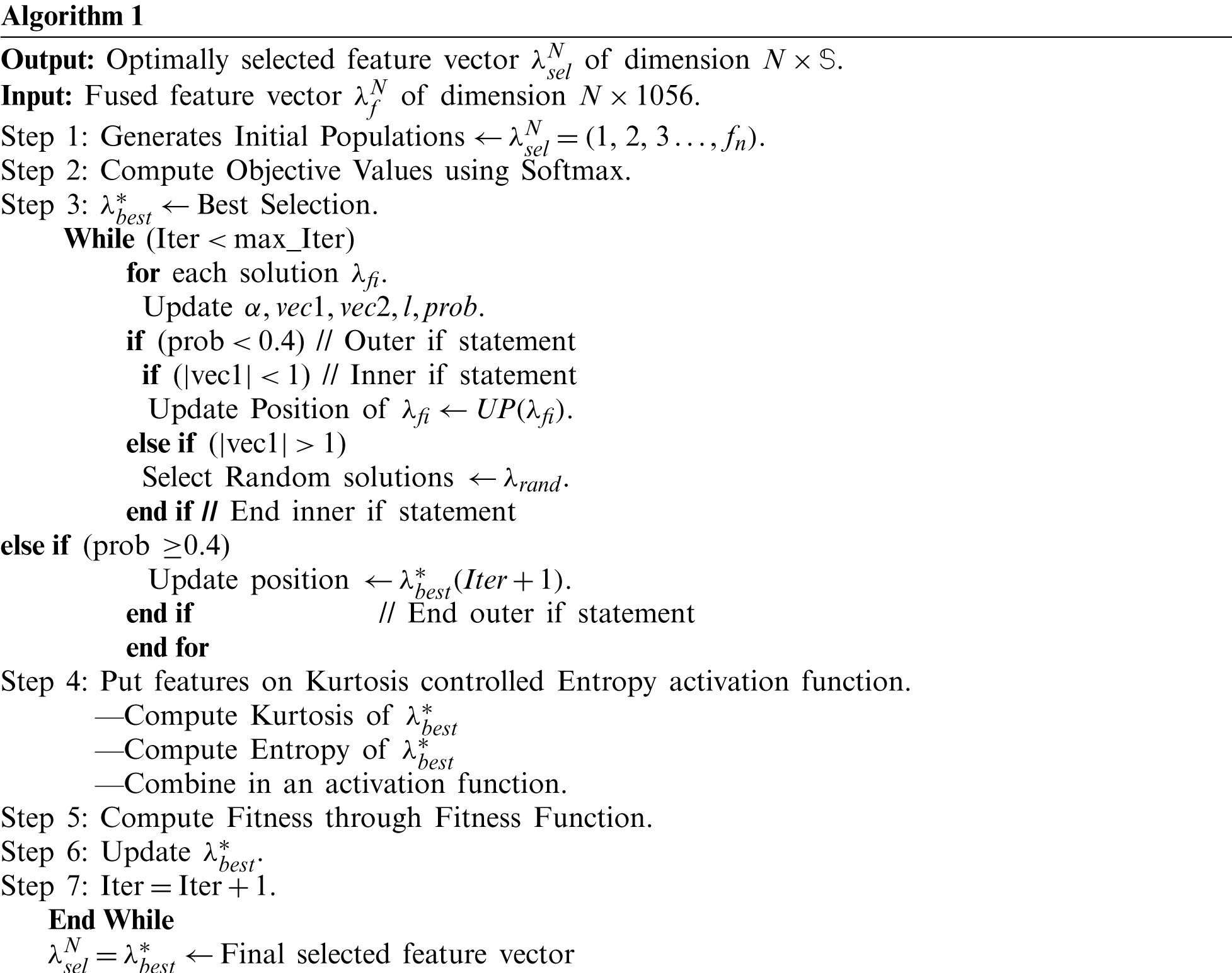
Whale Optimization Algorithm (WOA) [41] is a new optimization algorithm inspired to mimic the humpback whales’ natural behavior. Three main steps are involved in this algorithm: (i) prey encircling, (ii) exploitation, and (iii) exploration [42]. The detail of each step can be found in [41,42]. This algorithm is a wrapper-based approach because classification algorithms are applied to check the accuracy of selected features. In this paper, we used the Softmax classifier for classification accuracy.

Given a fused feature vector λfN of dimension N×1056 and λselN represents the selected optimal feature vector of dimension N×S, where S denotes the length of the optimally selected vector. Initially, we applied WOA, which returns the best features for each iteration. We add one more stage selection by a new activation function based on the Entropy and Kurtosis (E&K). Each iteration’s selected features are first passed in this function and then check the fitness through a fitness function. This process is continued until all initialized iterations are completed. The detail of this hybrid algorithm is given in Algorithm 1. In this algorithm, the maximum iterations (max_Iter) are 50, α is a parameter that decreases the linearly from 2 to 0, vec1 and vec2 are two coefficient vectors, l is a random number of range [ −1, 1], and prob is another random number of value between [0, 1]. In this algorithm, the position of whales is updated for prob<0.4 as follows:

UP(λfi)=λbest*(Iter+1)-vec1.Dist (26)

Dist=vec2.λbest*(Iter)-λfi(Iter) (27)

:

Here, Dist represents the distance among best selected features. The value of a random vector is between [0, 1]. For prob ≥0.4, the position is updated as follows:

λfi(Iter+1)=Dist′.ebl.cos(2πl)+λbest*(Iter)(28)

In the next, we proposed a new activation function for one more step feature selection. The activation function is defined as:

Funt=H(λbest*(Iter+1))×SK(λbest*(Iter+1))H(λbest*(Iter+1))+SK(λbest*(Iter+1))+0.1×Const (29)

Act(f)={G(λbest*(Iter+1)),forλbest*(Iter+1)i≥FuntNotConsider,Otherwise (30)

Based on this activation function, each selected feature is again checked and then compute the fitness through fitness function as follows:

Fitness=αEr(Dist)+b|R||f|(31)

Here, Er(Dist) represents the classification error, R represents the selected subset’s cardinality, and f represents the total features, respectively. This process is continued for maximum iterations, and at the end, we get a final optimal selected feature vector of dimension N×506. This vector dimension can be changed according to the nature of the dataset and selected iterations. Finally, the Softmax classifier [43] based classified these features for final classification. The proposed visual labeled results are shown in Fig. 7. The detailed testing results are discussed in Section 4.

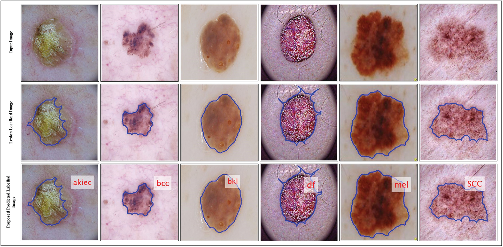
Figure 7: Proposed predicted labeled images

4  Experimental Results and Analysis

Experimental Setup: In this section, the proposed method results are presented. As shown in Fig. 2, the proposed method works through a sequence of steps. Therefore, we compute the results of each step to show the importance of the next step. As described in Section 3.1, three datasets are used for the experimental process; hence, we computed each datasets results with several experiments. The Softmax classifier is used as a main classifier in this work for the classification of selected features. The 70% of each dataset’s dermoscopic images are used to train a model, while the rest are used for testing. For cross-validation, we used 10-Fold validation. The performance of Softmax classifier is also compared with few other classifiers such as: Fine tree (F-Tree), Gaussian Naïve Bayes (GNB), SVM of cubic kernel function (C-SVM), extreme learning machine (ELM), fine KNN (F-KNN), and ensemble boosted tree (EBT). Each classifier performance is analyzed using the following performance measures such as sensitivity rate (Sen), precision rate (Prec) F1 Score, AUC, accuracy (Acc), and computational time. This work’s simulations are conducted on MATALB2020b using a Desktop Computer having 16 GB of RAM and 16 GB graphics card.

4.1 Results

Results of ISBI2018 Dataset: Tab. 1 presented the proposed classification results of multiclass skin lesions. The Softmax classifier produced the best performance of 97.1% accuracy rate using the proposed framework. The sensitivity and precision rate of Softmax is 86.34% and 97.41%, respectively. The F1-Score and AUC are also computed for this classifier, having obtained values are 91.54% and 0.987. The computational testing time is 21.627 (s). The C-SVM produced the second-best performance of 92.3% accuracy. The sensitivity, precision, and F-Score of this classifier are 77.07%, 84.40%, and 80.57%, respectively. For the rest of the classifiers, precision rate is 66.20%, 72.37%, 92.02%, 92.01%, and 92.65%. The minimum computational time is 7.9919 (s); however, it is noted that the accuracy of this classifier is almost 12% lesser as compared to Softmax. Moreover, the performance of the Softmax classifier is verified in Fig. 8 in the form of a confusion matrix. In this figure, it is illustrated that DF and VASC skin classes have high error rate. The main challenge in this work is an imbalanced dataset. Hence, due to low sample images, the error rate is high for these two classes.

Table 1: Proposed multiclass skin lesion classification results for ISBI2018 dataset

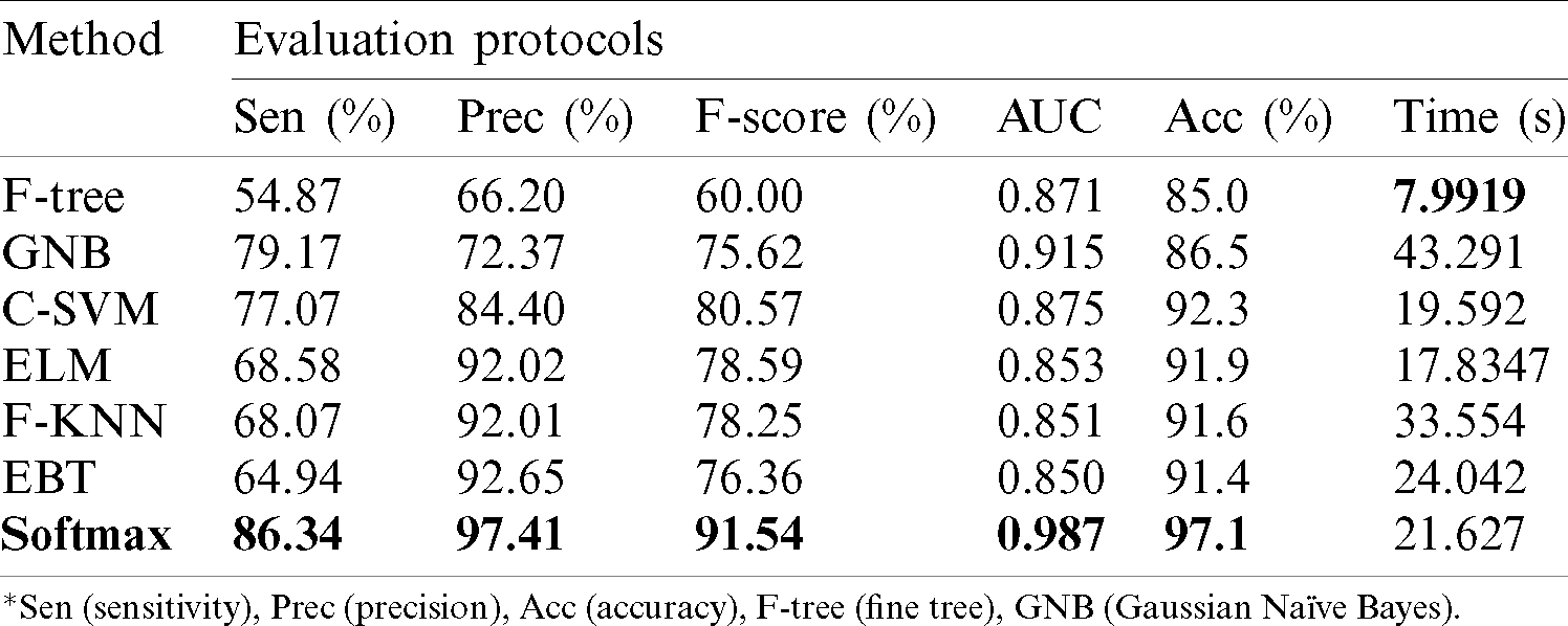
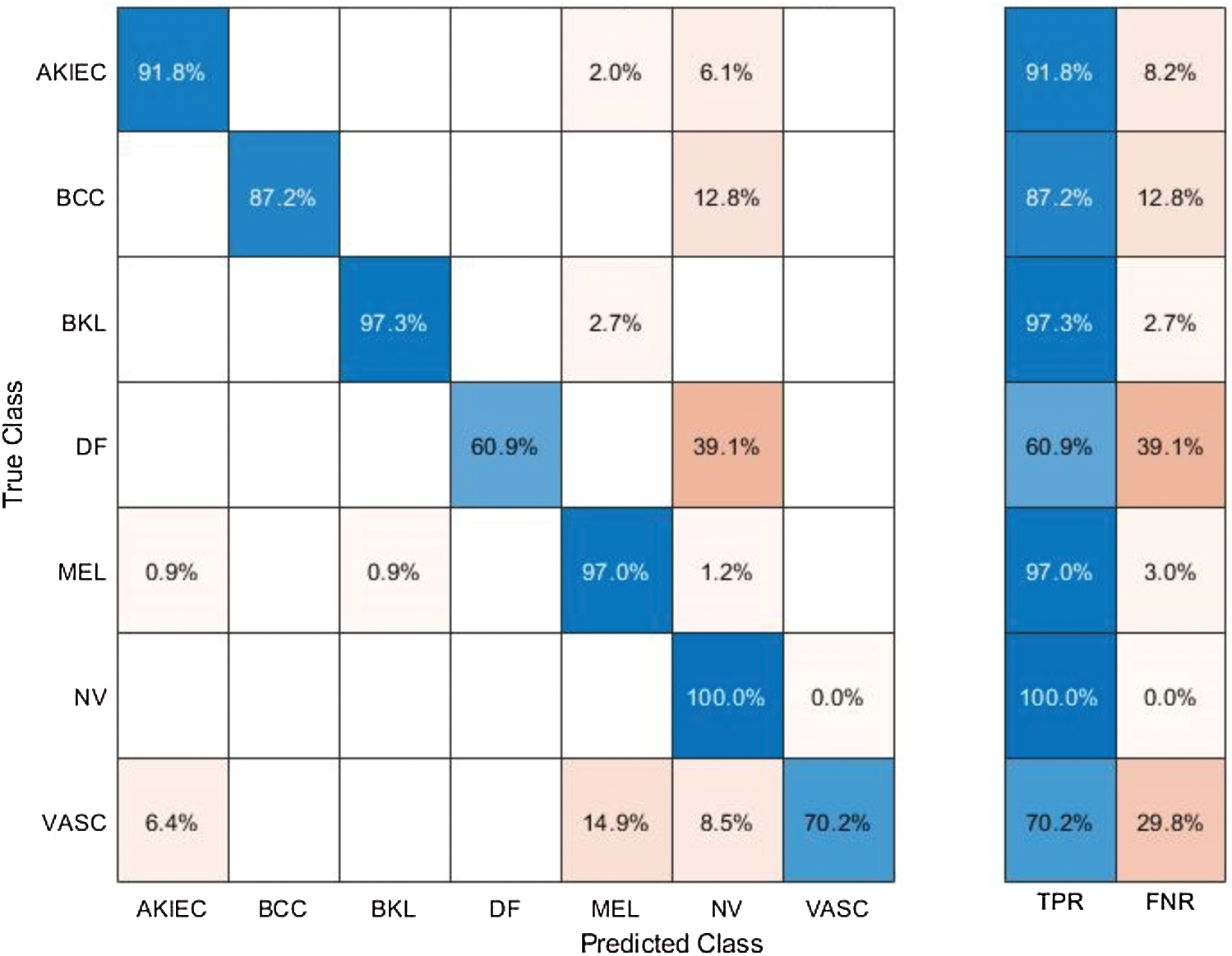
Figure 8: Confusion matrix of Softmax classifier using proposed method for ISBI2018 dataset

Tab. 2 presented the comparison of proposed framework accuracy with individual steps that are involved in this work. Initially, we computed the classification results without using lesion localization. The original images are directly passed in the proposed framework and achieved an accuracy of 90.8%, where the computational time was 16.1295 (s). In the second step, only Darknet53 is employed and performed experiment. For this experiment, the noted accuracy was 92.1%, but time is increased to 34.8915 (s). In the third step, results are computed for NasNet Mobile CNN and achieved an accuracy of 91.6%. In the fourth step, we removed the feature selection step and just fused features. For this experiment, the accuracy is improved to 94.2%, where the computational time was 24.1168 (s). In the last step, we consider the entire proposed framework and achieved an accuracy of 97.1% which is 7% improved as compared first step accuracy. The computational time of this experiment is 21.627 (s). Overall, it is noticed that the lesion localization step consumes much time, but this step improves the classification accuracy. Moreover, we compared the proposed accuracy with a few other neural nets, as illustrated in Fig. 9. From this figure, it is confirmed that proposed fusion and proposed selection methods outperform for this dataset.

Table 2: Comparison of proposed accuracy with individual steps

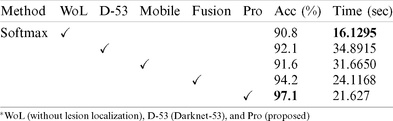
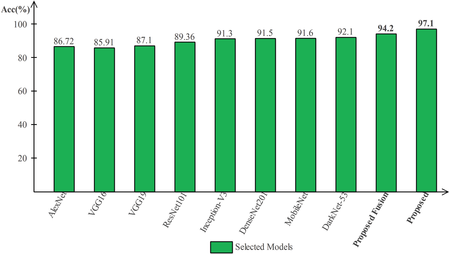
Figure 9: Comparison of proposed method with existing pre-trained deep learning models using ISBI2018 dataset

Results of ISBI2019 Dataset: Tab. 3 presented the proposed classification results of multiclass skin lesions using ISBI2019 dataset. The Softmax classifier produced the best performance of 85.3% accuracy rate using the proposed framework. The sensitivity and precision rate of Softmax is 73.3% and 82.6%, respectively. Moreover, the F1-Score and AUC are also computed for this classifier of 77.68% and 0.9725. The computational time of this classifier is 76.3046 (s). The GNB obtained the second-best performance of 84.9% accuracy. The sensitivity, precision, and F-Score of this classifier is 74.13%, 81.25%, and 77.53%, respectively. For the rest of the classifiers, the precision rate is 71.21%, 78.96%, 79.07%, and 82.59%. The minimum computational time is 61.112 (s); however, it is noted that the accuracy of this classifier is almost 9% lesser as compared to Softmax. Moreover, the performance of the Softmax classifier is verified in Fig. 10 in the form of a confusion matrix. This figure illustrated that BKL, DF, SCC, and VASC skin classes have low accuracy rates due to fewer images and high similarity.

Table 3: Proposed multiclass skin lesion classification results using ISBI2019 dataset

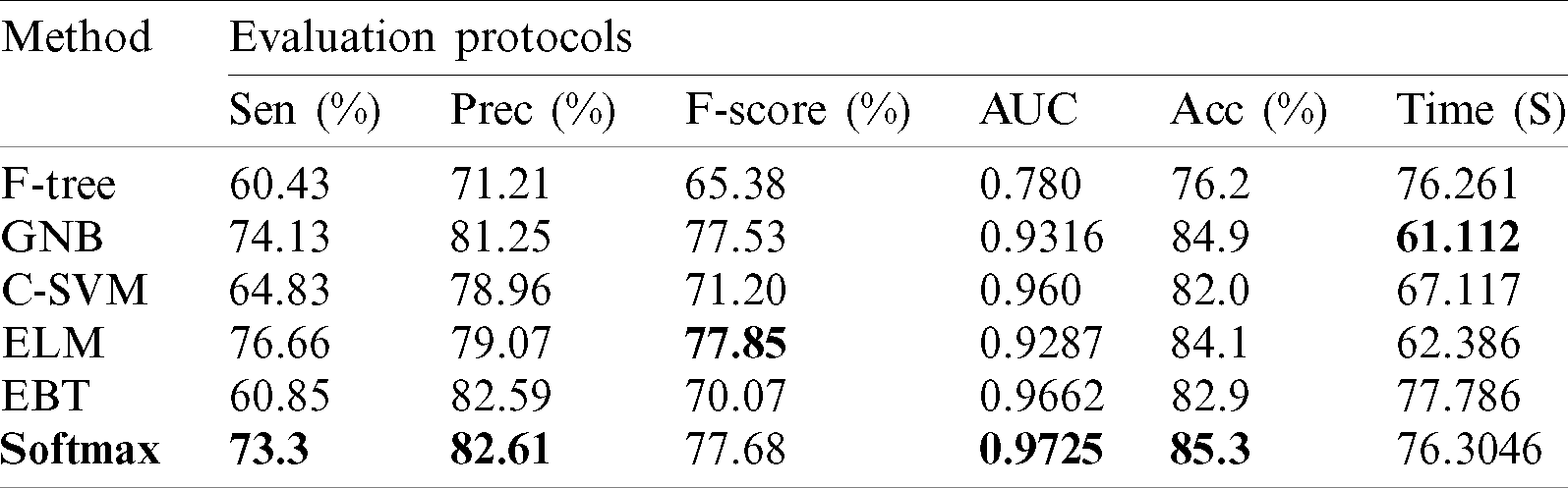
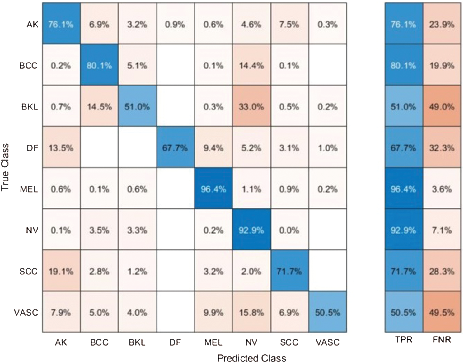
Figure 10: Confusion matrix of Softmax classifier using proposed method for ISBI2019 dataset

Tab. 4 presents the comparison of proposed framework accuracy with individual steps involved in the main Fig. 2. Initially, we computed the classification results without using lesion localization and obtained an accuracy of 78.6%, where the computational time was 39.448 (s). In the second step, only Darknet53 is employed and got an accuracy of 80.4%, but time is increased to 89.162 (s). This tie show that the lesion localization step consumes much time. In the third step, results are computed for NasNet Mobile CNN and achieved an accuracy of 81.9%. In the fourth step, we removed the feature selection step and just fused features of both networks. For this experiment, the accuracy is improved to 82.6%, where the computational time was 91.290 (s). In the last step, we consider the entire proposed framework and achieved an accuracy of 85.3%, which is 8% improved as compared first step accuracy and 3% from the fusion step. The computational time of this experiment is 76 (s). Overall, it is noticed that the lesion localization step is more important for improved classification accuracy. Also, the selection step minimizes the computational time and increases accuracy. Moreover, we compared the proposed accuracy with a few other neural nets, as illustrated in Fig. 11. This figure showed the significance of the proposed fusion and proposed selection steps for this dataset.

Table 4: Comparison of proposed accuracy with individual steps

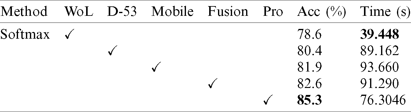
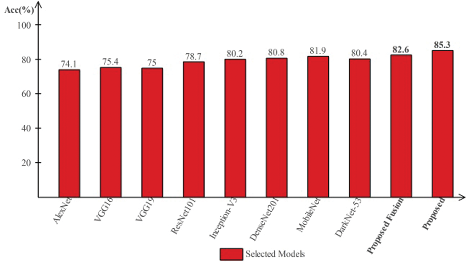
Figure 11: Comparison of proposed method with existing pre-trained deep learning models using ISBI2019 dataset

Results of HAM10000 Dataset: The proposed classification results of HAM10000 are presented in Tab. 5. This dataset’s best precision rate and accuracy are 92.22% and 95.8% for the Softmax classifier. The sensitivity rate is 84.20%, which can be verified in Fig. 12. This figure showed the confusion matrix of the Softmax classifier. Moreover, the F1-Score and AUC of this classifier are 88.03% and 0.9721. The computational time of this classifier is 9.546 (s). The second-best accuracy was achieved on CSVM of 94.9%. The sensitivity, precision, and F-Score of this classifier is 76.64%, 95.67%, and 85.10%, respectively. For the rest of the classifiers, the precision rate is 62.05%, 96.05%, 93.17%, 92.28%, and 93%. The minimum computational time is 8.189 (s) on F-KNN; however, it is noted that the accuracy of this classifier is almost 3% lesser as compared to Softmax, and there is no big difference in time among both. The comparison of proposed accuracy with an individual step involved in the proposed framework is presented in Tab. 6. From this table, the proposed accuracy is significantly better. Moreover, the proposed method accuracy is also compared with other neural nets, as illustrated in Fig. 13. This figure shows the significance of the proposed accuracy.

Table 5: Proposed multiclass skin lesion classification results using HAM10000 dataset

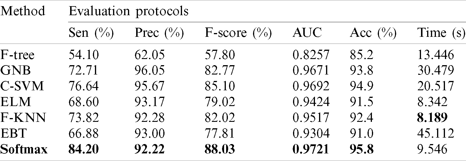
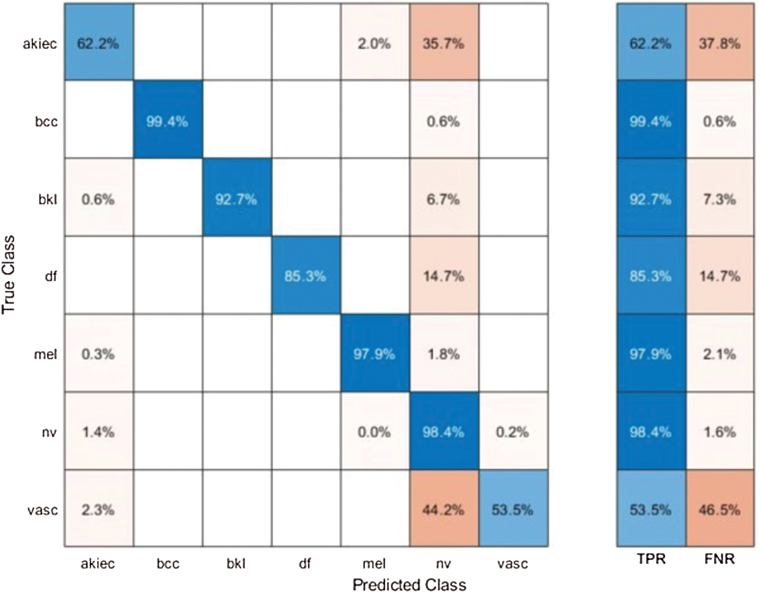
Figure 12: Confusion matrix of Softmax classifier using proposed method for HAM10000 dataset

Table 6: Comparison of proposed accuracy with individual steps using Ham10000 dataset

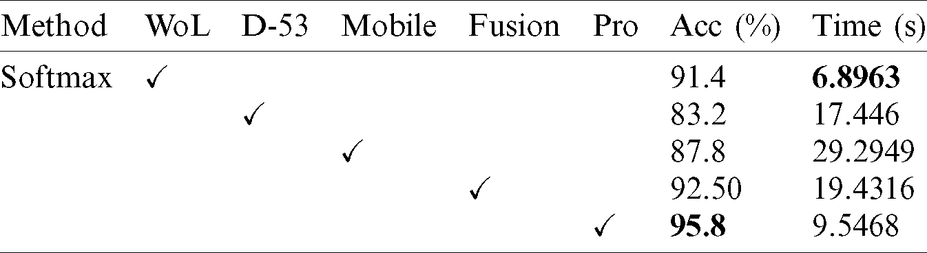
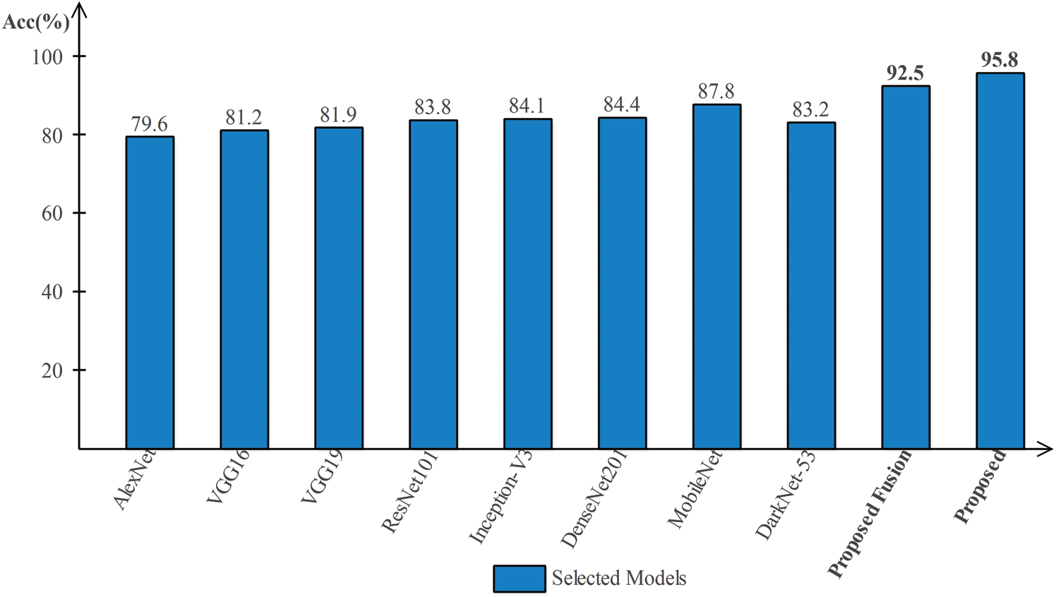
Figure 13: Comparison of proposed method accuracy with existing pre-trained deep learning models using HAM10000 dataset

4.2 Comparison

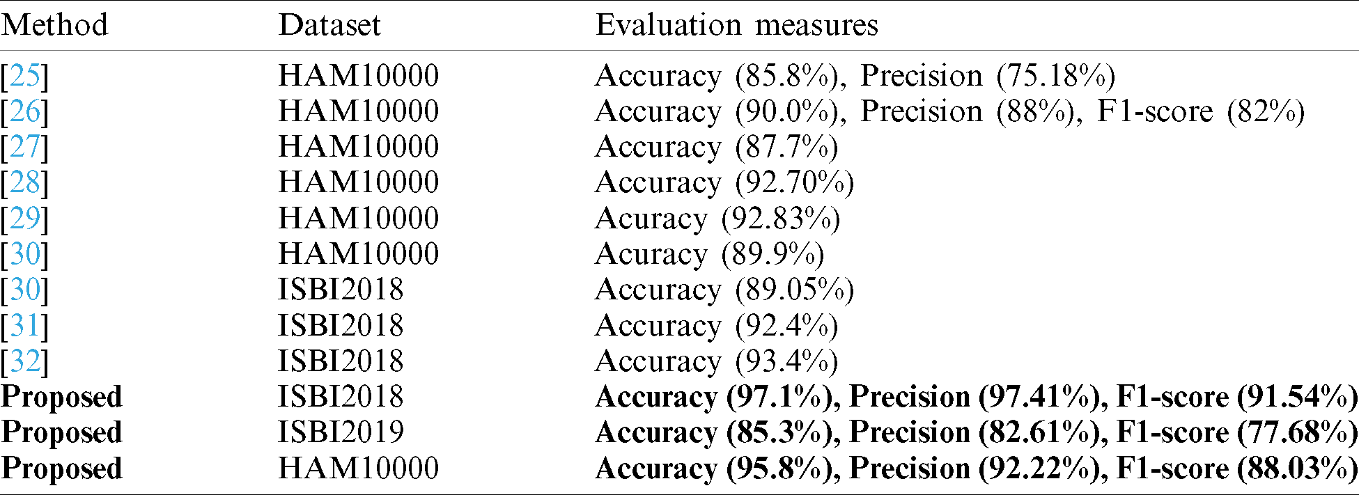
In this section, we analyze the proposed results based on the confidence interval and compare our proposed method accuracy with recent techniques as presented in Tabs. 7 and 8. In Tab. 7, it is described that a minor change is occurred in the accuracy after the 100 times execution of the proposed framework. Tab. 8, the each method is compared base on the dataset and evaluation measures. The accuracy is used as a main measure. However, few of them also consider precision and F1-Score. Hung et al. used the HAM10000 dataset and achieved an accuracy of 85.8% and a precision rate of 75.18%. Carcgani et al. noted accuracy was 90%, and F1-Score is 82%. However, our method obtained an improved accuracy of 95.8% and a precision rate of 92.22%. Similarly, for ISBI2018, the more recent best accuracy was 93.4%. Our method achieved an accuracy of 97.1%. For ISBI2019 dataset, our approach obtained an accuracy of 85.3%. From this table, it is shown that the proposed method works better on these selected datasets.

Table 7: Confidence interval based analysis of proposed accuracy

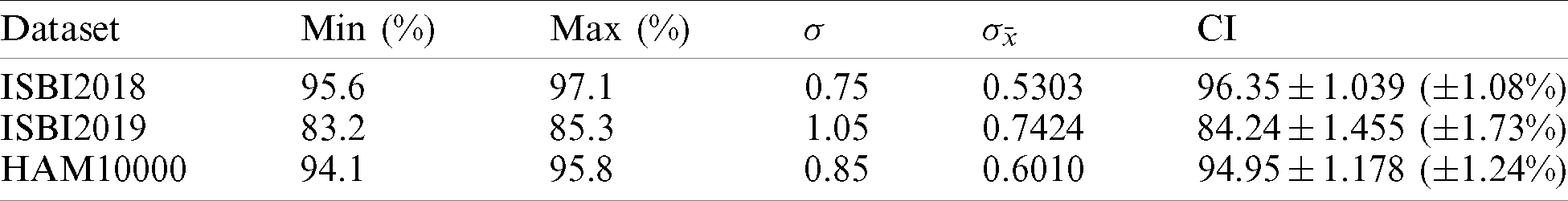
Table 8: Proposed method comparison with existing techniques

5  Conclusion

This paper presents a computerized architecture for multiclass skin lesion classification using a deep neural network. The main challenge of this work was imbalanced datasets for training a deep model. Therefore, in our method, we first localize the skin lesions for more useful feature extraction. This process improves the classification accuracy but increases the overall system computational time. The localized lesions are utilized for learning the pre-trained CNN models. The features are extracted from the last layers and performed fusion using a new parallel based approach. This approach’s main advantage is the fusion of most correlated features and controls the length of a feature vector. However, few redundant and irrelevant features are also added, which misclassifies the final classification accuracy. Therefore, we implemented a hybrid features optimization approach. The best features are selected using a proposed hybrid, which is finally classified using Softmax classifier. The experimental process is conducted on three extremely imbalanced datasets. On these datasets, our method achieved improved performance. This work’s main strength is the localization and fusion process; however, the selection of most optimal features decreases the computational time, as described in the results section. This work’s main limitation is the incorrect localization of skin lesion, which extracts the wrong features in the later stage. In the future, we will focus on the more optimized lesion localization approach, which is useful for real-time lesion localization and has improved accuracy.

Acknowledgement: Authors are like to thanks COMSATS University Islamabad, Wah Campus for technical support in this work.

Funding Statement: Authors are like to thanks COMSATS University Islamabad, Wah Campus for technical support in this work. This research was supported by Korea Institute for Advancement of Technology (KIAT) grant funded by the Korea Government (MOTIE) (P0012724, The Competency Development Program for Industry Specialist) and the Soonchunhyang University Research Fund.

Conflicts of Interest: The authors declare that they have no conflicts of interest to report regarding the present study.

This work is licensed under a Creative Commons Attribution 4.0 International License, which permits unrestricted use, distribution, and reproduction in any medium, provided the original work is properly cited.