Computers, Materials & Continua DOI:10.32604/cmc.2021.016372
Article

Local Stress Field in Wafer Thinning Simulations with Phase Space Averaging

Miaocao Wang1, Yuhua Huang1, Jinming Li1, Ling Xu2 and Fulong Zhu1,*

1School of Mechanical Science and Engineering, Huazhong University of Science and Technology, Wuhan, 430074, China
2School of Microelectronics, Fudan University, Shanghai, 200433, China
*Corresponding Author: Fulong Zhu. Email: zhufulong@hust.edu.cn
Received: 31 December 2020; Accepted: 05 February 2021

Abstract: From an ingot to a wafer then to a die, wafer thinning plays an important role in the semiconductor industry. To reveal the material removal mechanism of semiconductor at nanoscale, molecular dynamics has been widely used to investigate the grinding process. However, most simulation analyses were conducted with a single phase space trajectory, which is stochastic and subjective. In this paper, the stress field in wafer thinning simulations of 4H-SiC was obtained from 50 trajectories with spatial averaging and phase space averaging. The spatial averaging was conducted on a uniform spatial grid for each trajectory. A variable named mask was assigned to the spatial point to reconstruct the shape of the substrate. Different spatial averaging parameters were applied and compared. The result shows that the summation of Voronoi volumes of the atoms in the averaging domain is more appropriate for spatial averaging. The phase space averaging was conducted with multiple trajectories after spatial averaging. The stress field converges with increasing the number of trajectories. The maximum and average relative difference (absolute value) of Mises stress was used as the convergence criterion. The obtained hydrostatic stress in the compression zone is close to the phase transition pressure of 4H-SiC from first principle calculations.

Keywords: Local stress field; phase space; alpha shape; wafer thinning; molecular simulation

Symbols

Acronyms

1  Introduction

The shrinkage of semiconductor devices is posing challenges to semiconductor manufacturing processes. For one thing, dies are smaller, thinner and more fragile; for another, advanced packaging technologies such as 3D die stacking require high accuracy and consistency. To increase the quality and the yield, it is important to have a deep understanding on the manufacturing processes. As one of these processes, wafer thinning has attracted a lot of attention. At the nanoscale, wafer thinning has been studied as a scratching/grinding/cutting process with molecular dynamics (MD). Komanduri et al. [1] studied the effects of rake angle, clearance angle, depth of cut, and width of cut on the material removal and surface generation of monocrystalline silicon on nano-cutting. They found that silicon is undergoing pressure induced phase transformation from a diamond cubic structure to a body-centered tetragonal (bct) structure during the cutting process. Mylvaganam et al. [2] investigated the formation of nanotwins in monocrystalline silicon upon nano-scratching. When the scratch depth is greater than 1 nm, nanotwins emerges on the subsurface of silicon along 〈110〉 lattice direction and it is associated with the bct-5 phase transformation. Furthermore, the effects of residual stress and lattice orientation on the formation and stability of bct-5 silicon were investigated [3,4]. It showed that the hydrostatic stress component under the diamond tool plays an important role in the initiation of the bct-5 phase transformation The stable bct-5 silicon can only be generated by scratching on {001} crystal plane along 〈110〉 lattice direction and on {110} plane along 〈110〉 lattice direction at a scratch depth larger than 1 nm. A residual shear stress of 6–8 GPa is required to make bct-5 silicon stable. Ji et al. [5] compared the local stress distribution in nano-machining of silicon and copper, Li et al. [6] studied the effect of grinding speed on the subsurface damage thickness of silicon, and Guo et al. [7] studied the effect of multiple grinding on the thickness of damage layer. Recent thinning simulations on silicon concentrated on variations of the cutting tool, the substrate and the cutting trajectory [8–11]. In addition to silicon, the thinning process of silicon carbide (SiC) was also studied by researchers. Luo et al. [12] compared the machinability of different polymorphs of SiC by MD simulations. Comparing with 3C-SiC, 4H-SiC and 6H-SiC show lower cutting resistance. Tanaka et al. [13] performed the cutting test of surface modified SiC and conducted its nano-machining simulations with MD. The results showed that damage-free machining of monocrystalline SiC is possible by surface modification with an amorphous layer. Wu et al. [14] found the plastic deformation of 6H-SiC can be realized via phase transformation from the Wurtzite structure to an amorphous structure. These researches proved that molecular dynamics is a powerful tool on wafer thinning simulations.

The output of a MD simulation usually contains atoms’ position, atoms’ velocity, force related terms and energy related terms. To extract physical quantities like temperature and stress, post-processing on raw data is required. Many post-processing techniques on structural analysis have been developed such as radical distribution function (RDF), dislocation analysis (DXA) [15] and common neighbor analysis (CNA) [16]. As for the stress interpretation, it is still controversial since different equations on stress calculation have been put forward. Virial stress is the first local stress equation derived from virial theorem by Clausius [17]. Later, Irving et al. [18] obtained the stress tensor from equations of hydrodynamics with statistical mechanics. To avoid the Dirac function in Irving and Kirkwood’s equation, Hardy [19] introduced a localization function in the derivation of the stress equation. Tsai [20] traction was developed in the same period of time, based on the macroscopic definition of stress. Similarly, the stress vector on a plane for nano-indentation was acquired by Zhang et al. [21]. Recently, the widely used approach on stress calculation is the stress tally method [22] embedded in the Large-scale Atomic/Molecular Massively Parallel Simulator (LAMMPS) [23]. Other non-local stress equations were also utilized by some researchers [6,24]. To evaluate the stress state of the substrate during wafer thinning, the first issue lies in the choice of the stress equation. Different equations have different applicable conditions. Another issue is that, for a thinning simulation, the stress field calculated from a single phase space trajectory is stochastic and subjective. Based on the ergodic hypothesis that the time average equals to the ensemble average, for an equilibrium MD simulation, randomness and fluctuation can be eliminated with time averaging on a single phase space trajectory. However, the ergodic hypothesis does not hold for a non-equilibrium process. Different phase space trajectories have different stress field distributions.

To obtain the stress fields in thinning simulations of 4H-SiC, spatial averaging and phase space averaging were used. Different stress equations were briefly introduced and compared at first. Then, the MD thinning model of 4H-SiC, simulation details and some related algorithms were presented. The concept of phase space averaging was also illustrated. Finally, with different spatial averaging parameters, stress fields of 4H-SiC substrate on thinning were presented and discussed.

2  Comparison of Stress Equations

To calculate the stress state of a domain with N atoms, there are two branches, the virial-like stress equations and the Tsai traction equation. Virial, Hardy stress equations and LAMMPS stress tally method are virial-like stress equations with a virial term and a kinetic term. The virial term is the contribution of the interatomic forces in the domain and the kinetic term is the contribution of the momenta in the domain. The stress tensors from virial-like equations are symmetric. They describe the stress state of the domain. While the Tsai traction equation conducts stress calculation in a different way. It selects an area in the domain, accumulates the interatomic forces and momenta across the area in a short time period, and then divides the summation by the area and the time period. The stress vector from Tsai traction equation describes the stress state in the direction of the selected area. To obtain the stress state of the domain, Tsai traction equation should be conducted three times. Since Tsai traction equation depends on the selected area and the symmetry of its stress tensor is not strictly preserved, only virial-like stress equations were used and compared in this paper.

Virial stress equation [25] and Hardy stress equation [26] are given as follows,

σV=-1V[-12∑i,ji≠jNfij⊗rij¯+∑iNmivirel⊗virel¯] (1)

σH=-[-12∑i,ji≠jNfij⊗rijBij+∑iNmivirel⊗virelφi]Bij=∫01φ(λrij+ri-r)dλ (2)

where V is the volume of the averaging domain, N is the number of the atoms in the domain, rij=rj-ri, virel is the relative velocity of atom i with respect to the domain, ϕ is the localization function. Both equations were derived with a two-body potential assumption. For a many-body potential (2<Np≤4), two equations still hold with central force decomposition (CFD) and stress tensors are still symmetric and unique [25,27]. See Appendix A for a derivation of this.

The stress tally method in LAMMPS is given as follows,

σi=-[12∑i,jMII(fi⊗ri+fj⊗rj)+13∑i,j,kMIII(fi⊗ri+fj⊗rj+fk⊗rk)+mivi⊗vi](3)

where σi is in pressure×volume units; MII is the number of the force pairs (induced by a two-body potential) involving atom i; MIII is the number of the force sets (induced by a three-body potential) involving atom i. Unlike virial and Hardy stress equations, the per-atom stress tensor obtained with this method is an intermediate product. To speed up MD simulations, the virial terms are equally divided and assigned to the related atoms and spatial averaging is not included. With spatial averaging, LAMMPS stress equation is

σL=1V∑iNσi(4)

Fig. 1 is the illustration of virial, Hardy and LAMMPS stress equations with the same averaging domain. The black dot is the geometric center of the domain. The dashed line is the boundary of the domain. The yellow line is the virial contribution of an interatomic force. As shown in the figure, the virial contribution across the boundary is treated differently for three stress equations. In virial stress equation, that contribution is excluded. In Hardy stress equation, that contribution is partially included which depends on the localization function. In LAMMPS stress equation, half of that contribution is included. To reduce the ratio of the virial contribution around the boundary, a large domain is required for virial stress equation. Therefore, if the system is in equilibrium and the averaging domain is sufficiently large, virial stress equation is applicable. Hardy stress equation was derived from statistical mechanics. It is not limited to equilibrium systems. LAMMPS stress equation is the approximation to Hardy stress equation. Both equations are preferred for non-equilibrium simulations.

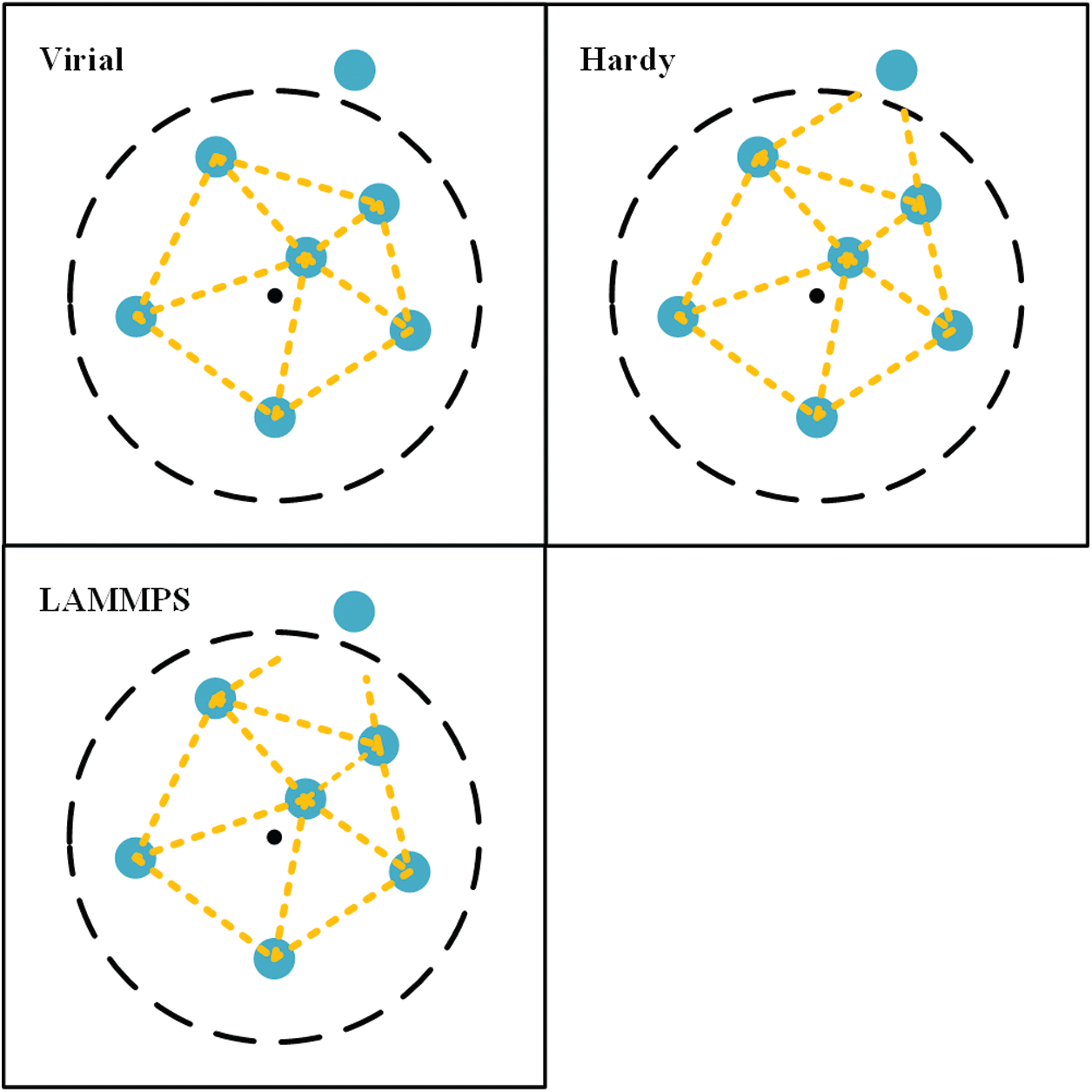
Figure 1: Illustration of three stress equations

3  Methodology

3.1 MD Simulation Model and Details

Fig. 2 shows the MD thinning model of 4H-SiC. The cutting tool is made of diamond. The 4H-SiC substrate consists of a fixed layer, an isothermal layer and a dynamic layer. The isothermal layer has a constant temperature of 300K. The cutting trajectory was along [011¯0] direction on (0001) plane. Tersoff potential [28] was used to describe the interatomic interactions. Other simulation details are listed in Tab. 1. The simulations were conducted with LAMMPS. The model and results were visualized by OVITO [29].

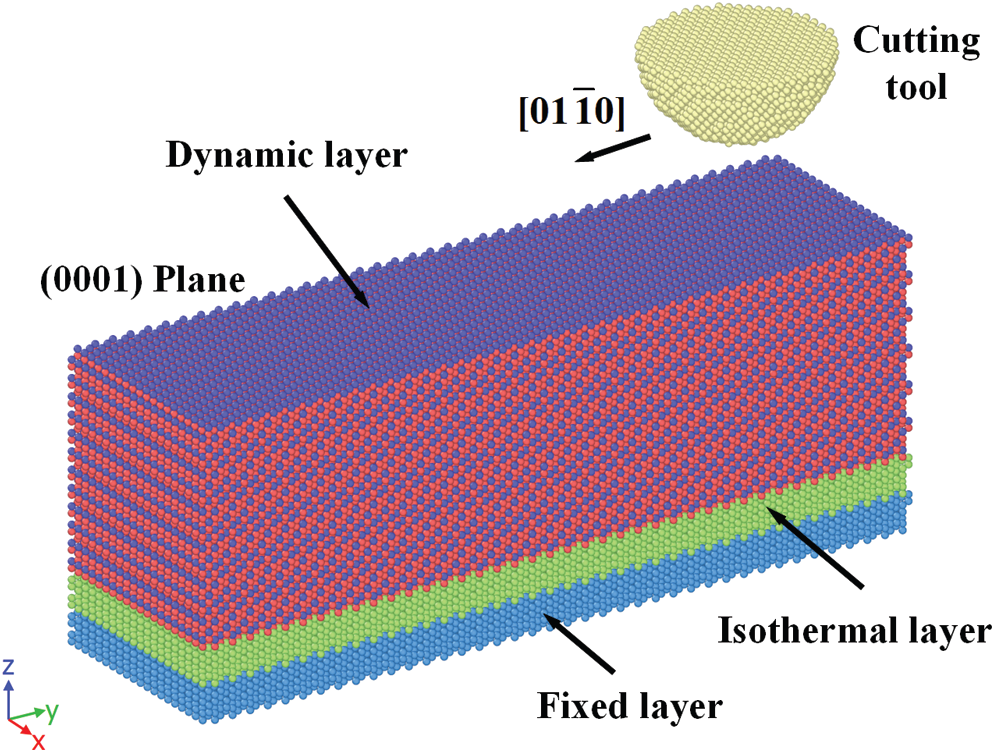
Figure 2: MD thinning model of 4H-SiC

Table 1: MD thinning simulation details

3.2 Spatial Averaging

The shape and the size of the averaging domain and the volume V in the stress equation are the main parameters in spatial averaging. A spherical domain and a cubic domain were used respectively. The spatial point was in the geometry center of the averaging domain, as shown in Fig. 3.

There are two simple ways to create spatial points. The first way is to use atoms’ position. It is straightforward since the data is directly accessible and the shape of the substrate is preserved. However, in this way, interpolation is inevitable in phase space averaging. The second way is to generate spatial points with a uniform spacing. It take slices in XYZ directions, the spatial point is the intersection of three slices, as shown in Fig. 3. Geometric features are lost but interpolation is avoided. The first way was used in the implementation of virial and Hardy stress equations in LAMMPS. The second way was used in the spatial averaging of LAMMPS stress equation outside LAMMPS.

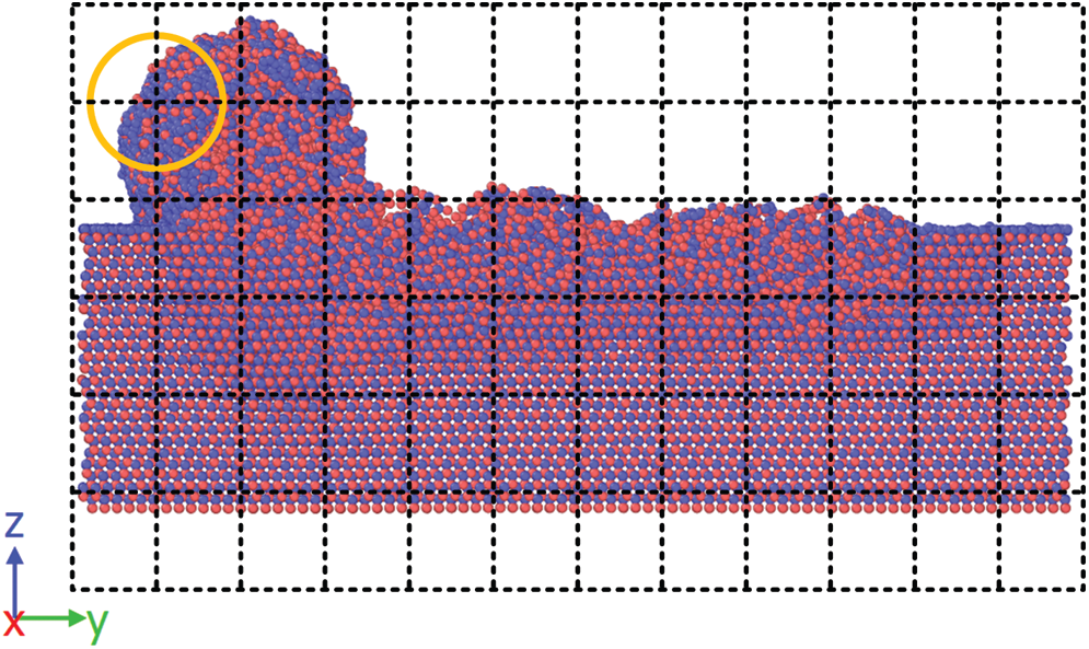
Figure 3: Illustration of spatial points and averaging domain

To overcome the shortage of geometric features and reconstruct the shape of the substrate in spatial points, alpha shape [30] algorithm was used. The alpha shape of a given set of atoms is a subset of its 3D Delaunay triangulation, controlled by the cutoff rc. The value of rc was a bit larger than the bond length of 4H-SiC in practice. Instead of removing the spatial points outside the alpha shape, a variable named mask was assigned to the points to indicate whether the point located in the alpha shape of the substrate. 3D Delaunay triangulation was achieved by the divide and conquer algorithm [31].

The size of the averaging domain is related to the number of atoms in the domain. According to the 4th numerical experiment in Admal’ work [25], a spherical domain with a diameter of 5–10 unit cells is appropriate for Face Centered Cubic (FCC) structure which has about 262–2094 atoms. Therefore, a domain with about 500 atoms was used.

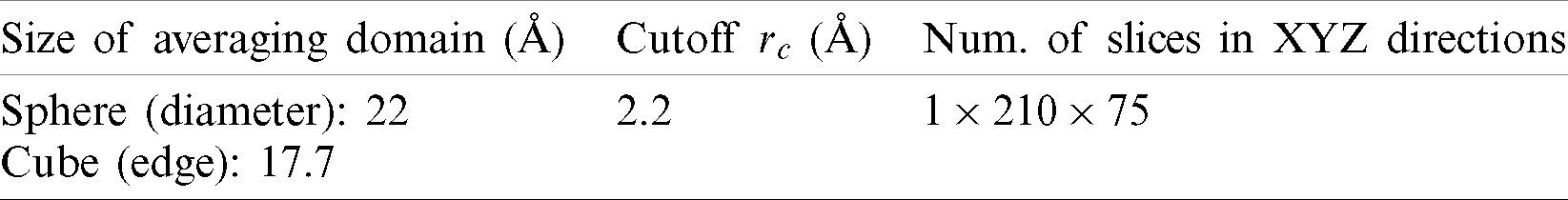
The volume V in the stress equation also has two choices. One is the volume of the averaging domain. The other is the summation of the Voronoi volumes of the atoms in the domain. By separating the related tetrahedrons generated from 3D Delaunay triangulation and then accumulating the related volumes, the Voronoi volume of each atom was obtained [32]. Parameters of spatial averaging are listed in Tab. 2.

Table 2: Spatial averaging parameters

3.3 Phase Space Averaging

For a system with NS atoms, its phase space is a 6×NS dimensional space which consists of all possible values of atoms’ position and momentum. A point in phase space is related to a microstate of the atoms. For a macrostate with a specific temperature/pressure/volume, there are many corresponding microstates. The MD simulation generates a trajectory in the phase space. It is the evolvement of the system’s configuration. It should be noted that a phase space trajectory is different from the cutting trajectory. Fig. 4a is the schematic of phase space and phase space trajectories [33]. For an equilibrium simulation, each point on the trajectory is related to the same macrostate (i.e., in the plane t = 0 in Fig. 4a). Therefore, the time averaging over a single trajectory is approximate to the ensemble averaging. For non-equilibrium simulations like thinning, different points on the same trajectory are related to different macrostates (i.e., the planes t = t1 and t = t2). The idea of phase space averaging is averaging trajectories from the same macrostate with different initial configurations, which is illustrated in Fig. 4b. Firstly, different velocity distributions were given to the same MD thinning model and then equilibration was conducted. The systems were around the same macrostate after equilibration. Then, the same thinning procedure was performed on these systems. After the thinning process, data at t = t1 was extracted for stress calculation. Stress field was calculated for each trajectory with spatial averaging. Finally, the average of the stress fields was obtained. To characterize the convergence of phase space averaging, the absolute value of relative difference of the von Mises stress between the (n −1)-th average and the n-th average was used. It was defined as

εS=|SMisesn-SMisesn-1SMisesn-1|(n>1)(5)

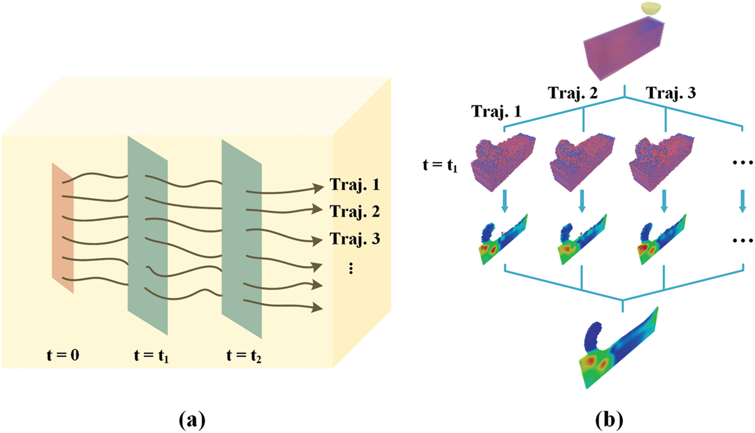
Figure 4: Illustration of phase space averaging. (a) Trajectories of non-equilibrium simulations. (b) Implementation of phase space averaging

4  Results

4.1 Comparison of Three Stress Fields

To find the appropriate stress equation for thinning simulations, hydrostatic stress fields calculated with virial, Hardy and LAMMPS stress equations are presented in Fig. 5. The averaging domain is a sphere with a diameter of 22 Å. The volume V in spatial averaging is the volume of the spherical domain. The localization function ϕ in Hardy stress equation has a constant value 1/V within the domain and equals zero outside the domain. Virial stress field was calculated without temporal averaging. Virial and Hardy stress equations were implemented with a user-defined fix style and a modified pair style in LAMMPS. The spatial averaging of LAMMPS stress equation was implemented outside LAMMPS with a script.

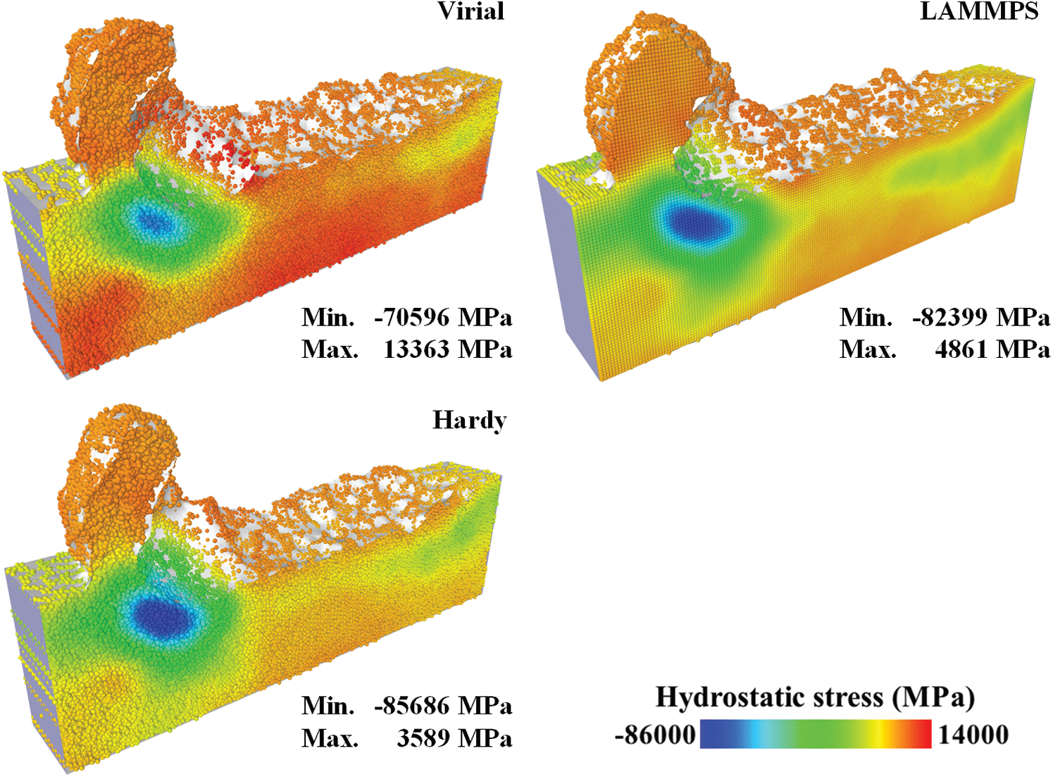
Figure 5: Hydrostatic stress fields with different stress equations (half model)

The spatial points in virial stress field and Hardy stress field consist of two parts, the atoms’ position and the center of the circumsphere of the tetrahedrons. The spatial points in LAMMPS stress field is a uniform grid. The points outside the alpha shape were removed. As displayed in the figure, three stress distributions are similar to each other, with a compression zone under the cutting tool. The difference lies in the value of the hydrostatic stress. Compared to the Hardy stress field, the stress value in virial stress field has a large bias (about 10 GPa). It indicates that the virial contribution of the interatomic forces across the boundary of the averaging domain is not negligible. The instantaneous version of virial stress equation is not suitable for stress calculation on thinning simulations. The LAMMPS stress field is approximate to the Hardy stress field. Considering the time cost, the LAMMPS stress equation was adopted in the following simulations.

4.2 Geometry Reconstruction

The purpose of introducing alpha shape algorithm was to reconstruct the shape of the substrate in the spatial grid. With the alpha shape, spatial points were divided into two groups, labeled by a variable named mask. In a single trajectory, the mask was either 0 or 1. After phase space averaging, the mask was a real number between 0 and 1. Fig. 6 shows the mask distribution from the average of 50 trajectories. Red points with a mask value of 1 are in the substrate, and blue points with a mask value of 0 at the top of the figure are outside the substrate. The region at the bottom of the figure where blue points occupied is the fixed layer and isothermal layer of the substrate. Since the atoms in that region were not taken into consideration in Delaunay Triangulation, the spatial points in that region have a mask value of 0. Apart from those red and blue points, there are some points in other colors, located on the surface of the substrate. The protuberance on the surface behind the cutting tool indicates that a cluster of atoms was adsorbed on to the cutting tool in some trajectories. With the variable mask, undesired spatial points were screened out, the shape of the substrate was reconstructed.

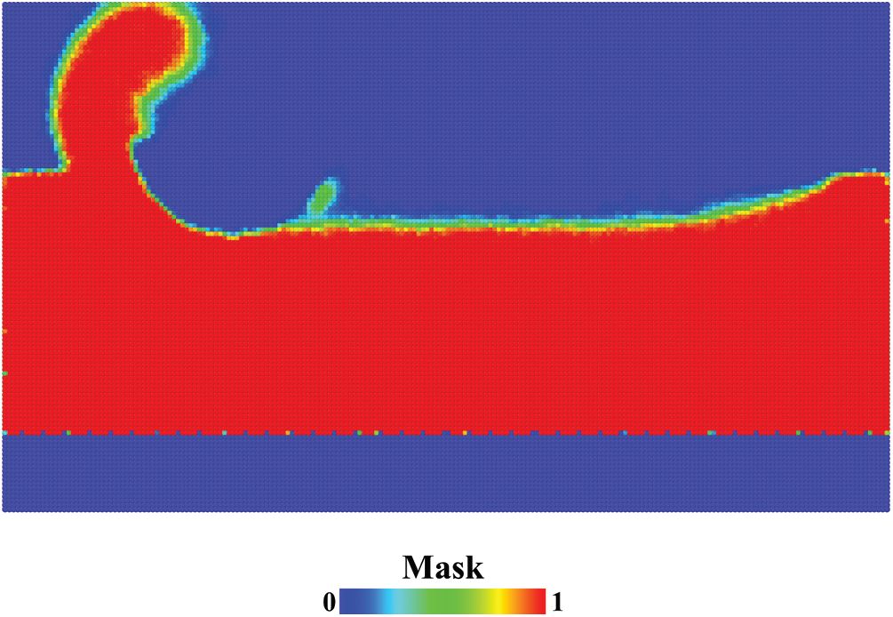
Figure 6: Mask distribution from the average of 50 trajectories

4.3 Convergence

Phase space average depends on the number of trajectories. To find an appropriate number of n, the absolute value of relative difference of Mises stress, i.e., εs, was calculated. Fig. 7 shows the distribution of εs with n equals to 50. Spatial points with a mask value less than 0.6 were removed. For most spatial points, εs is under 5%. For the spatial points located at the chip formed in the front of the cutting tool, εs is larger, with the maximum reached 7.74%. Fig. 8 shows the curves of maximum εs and average εs with respect to the number of trajectories. The pink line and the black line represent the maximum εs and average εs of all the displayed spatial points. Both relative differences decreased with increasing the number of trajectories. Compared to the maximum εs, average εs is smaller by one order of magnitude. The standard error of εs is about two orders of magnitude smaller than the average εs. When the number of trajectories reached 50, maximum εs is 7.74%, average εs is 0.36% and standard error is 0.00597%. With averaging over enough trajectories, the stress field converges. The number of trajectories, maximum relative difference and average relative difference can be used as a convergence criterion.

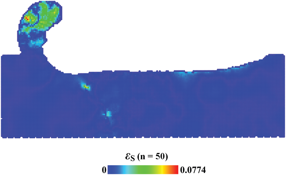
Figure 7: Distribution of relative difference of mises stress

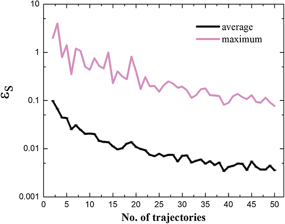
Figure 8: Relative difference of mises stress with respect to the number of trajectories

4.4 Stress Field Distributions

Mises stress fields and hydrostatic stress fields with different parameters are presented in Fig. 9. These fields were averaged over 50 trajectories. Different parameters were applied in spatial averaging. A spherical averaging domain was applied in Figs. 9b and 9c and a cubic averaging domain was applied in Fig. 9a. The volume of the spherical domain was used in Fig. 9c and the summation of the atoms’ Voronoi volumes was used in Figs. 9a and 9b.

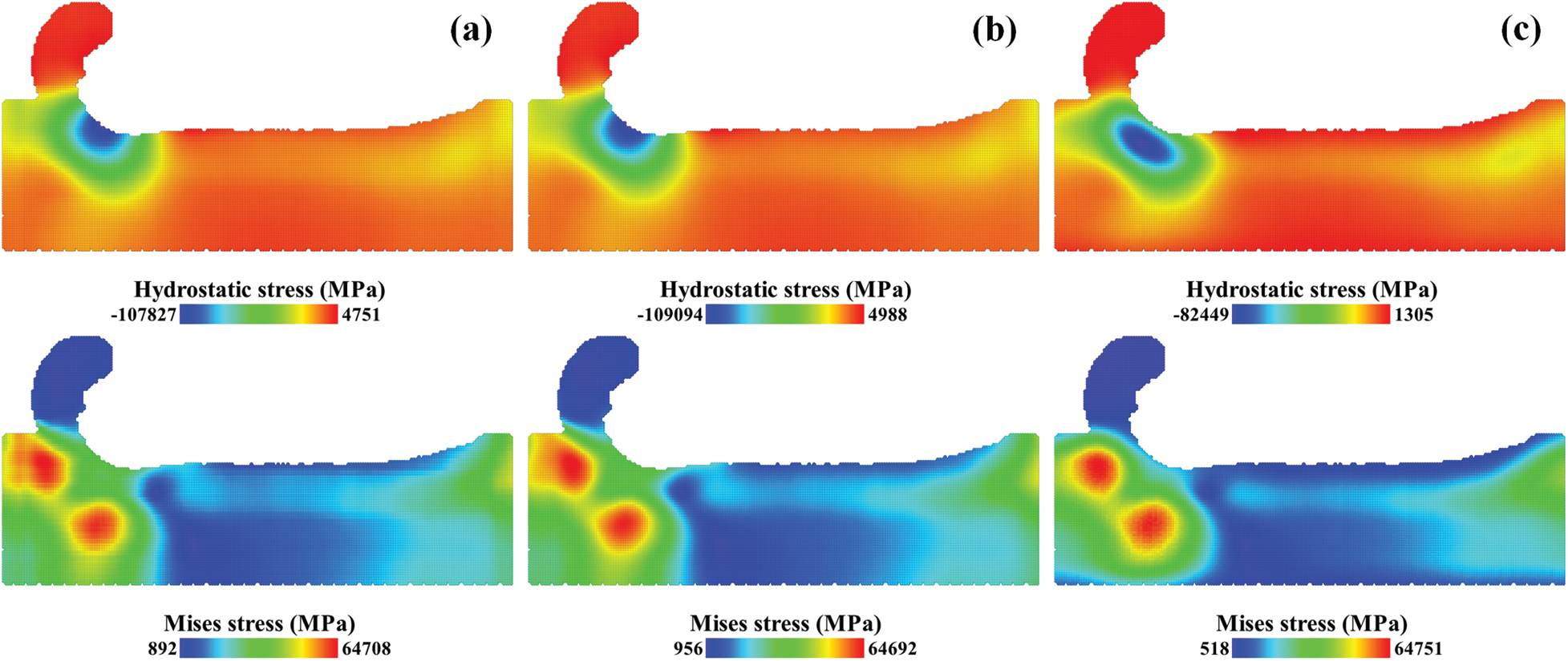
Figure 9: Mises stress fields and hydrostatic stress fields with different averaging parameters, (a) cubic domain with the summation of Voronoi volumes, (b) spherical domain with the summation of Voronoi volumes, (c) spherical domain with the constant volume

As we can see from the comparison of Figs. 9a and 9b, the stress distributions are similar and the stress values are close to each other. The compression zone is under the cutting tool with the maximum hydrostatic stress over 100 GPa. The stress fields with a spherical domain is smoother than the stress fields with a cubic domain, especially in the Mises stress field. When the number of the atoms in the averaging domain remains unchanged, the effect of the averaging domain’s shape on the stress field is limited. From the comparison of Figs. 9b and 9c, the stress fields with a constant volume in Fig. 9c have smaller stress values and different stress distributions. The compression zone has shifted into the substrate with the maximum hydrostatic stress reduced to 82 GPa. The difference concentrates on the surface of the substrate. As shown in Fig. 10, the spatial point in the center of the substrate has a volume of 5722 Å3 which is close to the volume of the spherical domain, whereas the spatial point on the surface has a much smaller volume. With a large bias on volume V, the stress values on the surface in Fig. 9c were underestimated.

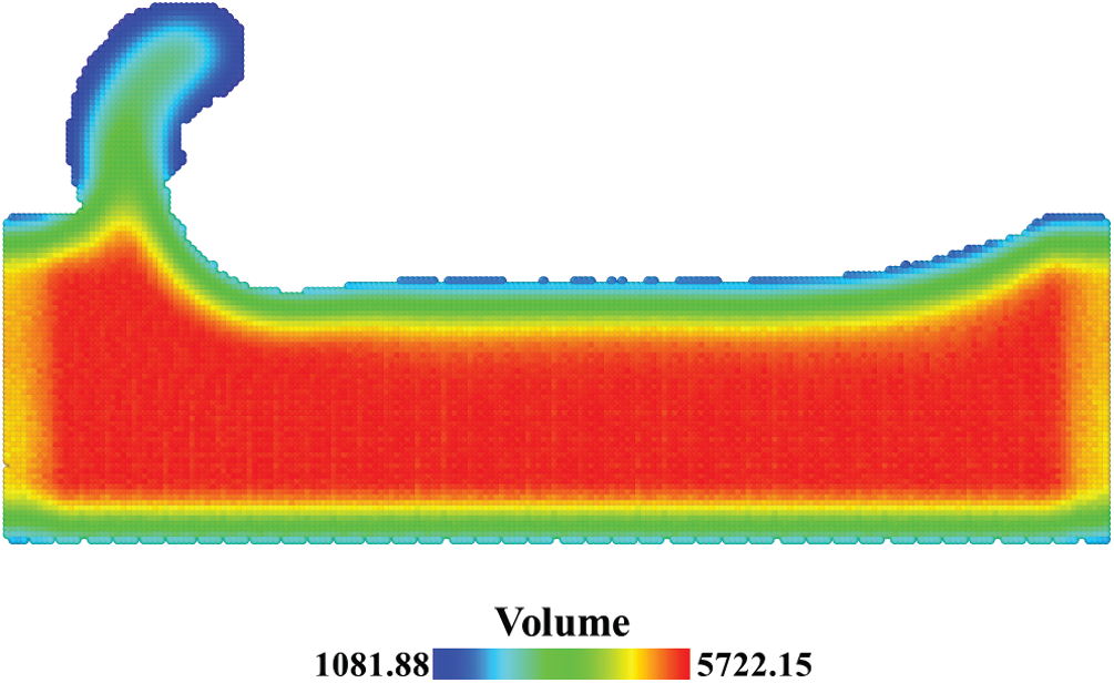
Figure 10: Distribution of the summation of Voronoi volumes in the averaging domain

4.5 Temperature Field Distribution

With atoms’ velocity, the local temperature field was extracted and averaged over 50 trajectories. It was calculated by the following equation [34],

Ek=∑iN12mivirel⋅virel=32NkT(6)

where k is the Boltzmann constant. The temperature field is presented in Fig. 11. The high temperature zone is located at the chip formed in the front of the cutting tool with the maximum temperature reached 2797 K. The relative difference (absolute value) of the temperature was also calculated. When the number of trajectories reached 50, maximum relative difference is 0.327%, average relative difference is 0.0649% and standard error is 0.000454%.

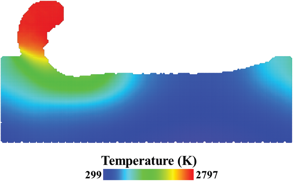
Figure 11: Temperature field from the average of 50 trajectories

5  Discussion

The virial-like stress equations are identical in the thermodynamic limit. With a large number of atoms in the averaging domain, the virial contribution of the forces across the boundary is negligible. However, the averaging domain is far away from the thermodynamic limit in practice. Virial and Hardy stress equations have different treatments on the virial contribution of the forces across the boundary. The contribution is discarded in the virial stress equation, which leads to its heavy dependence on the size of the averaging domain. While in Hardy stress equation, the contribution is taken into account by the localization function. Although Hardy stress equation is suitable for thinning simulations, the time cost is huge. To speed up the simulation, the virial contribution of the interatomic forces is equally divided and assigned to the related atoms in LAMMPS. In this way, the time cost on the spatial averaging was reduced from hours to minutes since the number of interatomic forces (O(NS2)) is much larger than the number of atoms (O(NS)).

Spatial averaging was used to extract the stress field from a single trajectory. The effect of the averaging domain’s size was investigated in Admal’s work [25]. With increasing the size of the domain, more atoms are involved in the stress calculation and the obtained stress tensor is more reliable. However, microscopic stress fields are often computed for small systems (limited by the hardware). If the size of the domain is comparable to the system size, the stress tensor is more like a global value. The effect of the averaging domain’s shape on the stress field is limited when the number of atoms in the domain is fixed. While the volume V has a great influence on the stress value of the spatial points around the surface. For those spatial points around the surface, when the constant volume of the spherical domain was applied, the stress value was underestimated. This may account for the drop-off of Hardy stress around the hole in Admal’s numerical experiment [25]. Phase space averaging was introduced to average the stress fields from different trajectories. Although the phase space average is not strictly equal to the ensemble average, the stress field obtained from phase space averaging converges. The maximum relative difference and the average relative difference of Mises stress and the number of trajectories could be used as a convergence criterion. The maximum hydrostatic stress of 4H-SiC substrate on thinning is 109 GPa which is in agreement with the phase transition pressure of 100 GPa from the ab initio experiment [35].

6  Conclusions

This paper aims to obtain the local stress field objectively from the MD trajectories and provide an alternative to the stress calculation of wafer thinning simulations. The stress field in thinning simulations of 4H-SiC was obtained from 50 trajectories with spatial averaging and phase space averaging.

The spatial averaging was conducted on a uniform spatial grid. To reconstruct the shape of the substrate, a variable named mask was assigned to the spatial point. The averaging domain was a sphere with a diameter of 22 Å for 4H-SiC. Compared with the constant volume of the spherical domain, the summation of the Voronoi volumes of the atoms in the domain is more appropriate in spatial averaging since the stress value around the surface of the substrate was underestimated with the constant volume.

The phase space averaging was conducted after spatial averaging. The stress field converges with increasing the number of trajectories. The relative difference (absolute value) of Mises stress was used to characterize the convergence of the phase space averaging. When the number of trajectories reached 50, the maximum and average relative difference (absolute value) of Mises stress is 7.74% and 0.36%. The maximum hydrostatic stress in the compression zone of 4H-SiC substrate has reached 109 GPa. It is close to the ab initio result of 100 GPa.

Funding Statement: This work was supported by National Natural Science Foundation of China (52075208), National Natural Science Foundation of China (U20A6004), National Natural Science Foundation of China (Number: 51675211) and Shanghai Municipal Science and Technology Major Project (No.2018SHZDZX01) and ZJLab.

Conflicts of Interest: The authors declare that they have no conflicts of interest to report regarding the present study.

Appendix A. Derivation of Stress Tensor’s Symmetry and Uniqueness

The interatomic potential E is a function of relative distances rαβ for most parametric potentials such as Lennard–Jones (LJ), Stillinger–Weber (SW), and Tersoff potentials. For a Np-body potential,

E=E(rαβ)(A1)

where α,β=i,j,k…︷N and α≠β. The interatomic force on atom α is

fα=-∂E∂rα(A2)

With the chain rule, it can be written as

fα=-∂E∂rα=-∑β∂E∂rαβ∂rαβ∂rα(A3)

In Cartesian coordinates, relative distance rij can be expressed as

rij=|rj-ri|=(xj-xi)2+(yj-yi)2+(zj-zi)2(A4)

and its partial derivative to vector ri can be written as

∂rij∂ri=(∂rij∂xi∂rij∂yi)(A5)

Substituting (A4) into (A5), with simplification, we have

∂rij∂ri=(xi-xjrijyi-yjrij)=-r^ij(A6)

where r^ij is the unit vector in the direction of rij. Similarly,

∂rij∂rj=r^ij(A7)

Substituting (A6) to (A3), we have

fα=-∑β∂E∂rαβ∂rαβ∂rα=∑β∂E∂rαβr^αβ(A8)

where α,β=i,j,k…︷N and α≠β. It should be noted that ∂E∂rαβ is the result of a Np −2 times multiple summation for many-body potential (Np > 2). When Np = 4, put i, j, k, l into α,β, we have

fi=∑j∂E∂rijr^ij+∑k∂E∂rikr^ik+∑l∂E∂rilr^ilfj=-∑i∂E∂rijr^ij+∑k∂E∂rjkr^jk+∑l∂E∂rjlr^jlfk=-∑i∂E∂rikr^ik-∑j∂E∂rjkr^jk+∑l∂E∂rklr^klfl=-∑i∂E∂rilr^il-∑j∂E∂rjlr^jl-∑k∂E∂rklr^kl(A9)

Obviously, fα can be decomposed at the position of atom α in three directions, and this decomposition is unique as long as three unit vectors are linearly independent. This decomposition is named Central Force Decomposition (CFD). When Np is larger than four, the number of unknown variables is larger than the number of equations (Np −1 > 3), variables are not set until new constraints introduced.

With CFD, the components of the interatomic forces can be arranged pair by pair like “virtual” bond. The contribution of these “virtual” bonds to the virial term in the stress tensor is,

fαβ⊗rα+fβα⊗rβ=-∂E∂rαβr^αβ⊗rαβ(A10)

Thus, the symmetry of the stress tensor is preserved.

In summary, for Np-body potential which is a function of the atoms’ relative distances, when Np < 5, the symmetry of the stress tensor can be preserved with Central Force Decomposition.

This work is licensed under a Creative Commons Attribution 4.0 International License, which permits unrestricted use, distribution, and reproduction in any medium, provided the original work is properly cited.