Computers, Materials & Continua DOI:10.32604/cmc.2021.016663
Article

Learning Unitary Transformation by Quantum Machine Learning Model

Yi-Ming Huang1, Xiao-Yu Li1,*, Yi-Xuan Zhu1, Hang Lei1, Qing-Sheng Zhu2 and Shan Yang3

1School of Information and Software Engineering, University of Electronic Science and Technology of China, Chengdu, 610054, China
2School of Physics, University of Electronic Science and Technology of China, Chengdu, 610054, China
3Department of Chemistry, Physics and Atmospheric Sciences, Jackson State University, Jackson, MS, 39217, USA
*Corresponding Author: Xiao-Yu Li. Email: xiaoyuuestc@uestc.edu.cn
Received: 08 January 2021; Accepted: 09 February 2021

Abstract: Quantum machine learning (QML) is a rapidly rising research field that incorporates ideas from quantum computing and machine learning to develop emerging tools for scientific research and improving data processing. How to efficiently control or manipulate the quantum system is a fundamental and vexing problem in quantum computing. It can be described as learning or approximating a unitary operator. Since the success of the hybrid-based quantum machine learning model proposed in recent years, we investigate to apply the techniques from QML to tackle this problem. Based on the Choi–Jamiołkowski isomorphism in quantum computing, we transfer the original problem of learning a unitary operator to a min–max optimization problem which can also be viewed as a quantum generative adversarial network. Besides, we select the spectral norm between the target and generated unitary operators as the regularization term in the loss function. Inspired by the hybrid quantum-classical framework widely used in quantum machine learning, we employ the variational quantum circuit and gradient descent based optimizers to solve the min-max optimization problem. In our numerical experiments, the results imply that our proposed method can successfully approximate the desired unitary operator and dramatically reduce the number of quantum gates of the traditional approach. The average fidelity between the states that are produced by applying target and generated unitary on random input states is around 0.997.

Keywords: Machine learning; quantum computing; unitary transformation

1  Introduction

With the enormous variety of applications, machine learning has already impacted modern life [1,2]. It not only provides powerful tools for mining the potential information from massive data but also helps us explore the laws of nature from a new perspective. In recent years, machine learning has caught the attention of researchers from various fields such as physics and chemistry [3,4]. They intend to develop new tools based on machine learning techniques for scientific research. Quantum machine learning is one such rising and promising branch that combines the approaches of data processing from machine learning with the outperformance of quantum computing. As well known, there is computational difficulty in simulating a quantum system by classical methods. As the size of a quantum system increases, the resources required for simulating will increase exponentially.

Based on this fact, quite a lot of quantum machine learning models that harness the quantum advantages have been proposed in recent years. Quantum support vector machine (QSVM) and its physical implementation that runs on a small-scale quantum device result in an exponential speed-up over the corresponding classical one [5]. Quantum principal component analysis (QPCA) is more than a quantum extension of the classical algorithm. It also provides a technique to construct unitary transformation efficiently [6]. Quantum generative adversarial networks (QGAN) inherit the framework of classical models, consisting of a generator and a discriminator. However, the components of QGAN can be constructed by variational quantum circuits such that generating quantum data is more efficient like quantum state preparation [7–10]. These quantum machine learning models are classified into two categories. One category is full quantum that the models only rely on full quantum algorithms including quantum Fourier transformation, quantum phase estimation and HHL algorithm etc. [11,12]. The representative works are QSVM, QPCA, and so on. Another category is hybrid that the models consist of the classical part and quantum part. That is the reason why it is called the hybrid quantum-classical model. These models are formalizing the problem of interest as a variational optimization problem and finding an approximate solution by parametrized quantum circuit and classical optimizer [13]. Compared to the full quantum-based model, the hybrid quantum-classical model requires fewer resources to build, particularly the size of the quantum system, the number of quantum gates, etc. Meanwhile, the well-developed optimization techniques can be naturally employed, which means that we are able to make use of well-maintained open-source optimization libraries such as Tensorflow and Pytorch as the optimizing backend [14,15].

In this work, relying on the advantages of the hybrid-based quantum machine learning model, we intend to exploit it for a unitary learning problem that is an essential task in quantum computing. One reason why learning unitary matrices matters a lot is that the dynamics of a quantum system can be described by a unitary transformation, exploring the efficient way to implement the unitary transformation is fundamental. Since we are still in the early stages of quantum computing with the limitation of quantum resources for computation, it is necessary to investigate how to control or manipulate the quantum system efficiently. Besides, various tasks will benefit from the results of the study on learning unitary transformation. For instance, unitary matrix compiling, that is the task of ‘compiling’ a known unitary transformation into a quantum circuit constructed by a sequence of gates chosen from the specific quantum gate set. A large amount of existing works has been focused on how to implement unitary transformations efficiently. Such works provide theoretic analysis of approximate error and gate or time complexity for implementing target unitary transformation [16,17]. Recently, some work investigated the ideas from machine learning for simulating a desired unitary transformation [18,19]. Similar to these related literatures, we formulate the learning of a given target unitary operator as an optimization problem, and employ the hybrid-based quantum machine learning model to approximate the solution. From our numerical experiments, the results show that the proposed method provides a reasonable approximation while the number of required quantum gates is much less than those of traditional approach.

We organized this paper as follows. In Section 2, we formalize the learning problem of unitary transformation. In Section 3, we give a brief introduction of the techniques in hybrid quantum-classical framework and quantum generative adversarial networks (QGAN). In Section 4, we propose a method by which a quantum machine learning model can be used for solving the formulized unitary learning problem. In Section 5, we provide the numerical experiments which demonstrate the advantages of the proposed model. We also introduce the background of quantum computing in the appendix.

2  Learning Problem of Unitary Transformation

In quantum mechanics, we have two pictures for the dynamics of a quantum system. One is the Hamiltonian picture; another is the unitary operator picture. In the Hamiltonian picture, given the Hamiltonian, a Hermitian operator, that is the total energy function of the closed system, we can describe the evolution of the system by Schrödinger equation as follow,

iℏd|φ〉dt=H|φ〉(1)

It can be verified that the solution of Eq. (1) can be,

|φt2〉=e-iℏH(t2-t1)|φt1〉=U|φt1〉(2)

Because the Hamiltonian H is a Hermitian operator, the operator U is unitary. Thus, in the unitary operator picture, we use this unitary transformation to formulate the quantum dynamics.

U=e-iℏ⋅H⋅t(3)

In the following, our discussion is mainly under the unitary operator picture. As shown in Eq. (2), the manipulation of a quantum system is equivalent to manipulating corresponding unitary matrices. Once there is an efficient way to implement the desired unitary operator, we can effectively imitate the behavior, that is the dynamics, of a quantum mechanical system, which is an intractable task for classical methods [20]. This learning unitary problem introduced above is related to Hamiltonian simulation, which suppose given a Hamiltonian H, time t and precision ε>0, the task is to find a quantum algorithm (quantum circuit) to produce operator U which is approximate to the target unitary operator UT=e-i⋅H⋅t, that is,

|UT-Ũ|≤ε(4)

Plenty of methods were proposed in past years. Lloyd [20] first invented the quantum algorithm by using Lie-Trotter product formula for simulating Hamiltonian which only includes the local interactions. Berry et al. [21] based on Trotter–Suzuki algorithm gave a method for simulating sparse Hamiltonian. As the unitary operator can be rewritten by the Taylor series expansion, Berry et al. [22] gave an algorithm for approximating the unitary operator with the truncated Taylor series in the same year. Low et al. [23] proposed a quantum signal processing for simulating. Being different from these approaches by quantum algorithm, some works intended to build a unitary operator by neural network or parametrized quantum gate sequence to approximate the target [19,24]. They formulize the approximation of the target evolution operator as an optimization problem. The loss function is the square of Frobenius norm between desired unitary operator and parametrized alternating operator sequences [19].

3  Quantum Machine Learning

In this section, we will introduce the hybrid-based quantum machine learning model. The hybrid quantum-classical framework is derived from the quantum approximate optimization algorithm (QAOA) [25]. The QAOA was proposed for solving the MAX-CUT problem, which can be viewed as minimizing the expectation value of a specific observable A that encodes the subjective function in the parametrized quantum state generated by applying alternating operators e-iβi⋅B and e-iγi⋅A on a uniform quantum state as follow,

minβ,γ〈A〉=tr(A⋅ρβ,γ)=〈β,γ∣A∣β,γ〉(5)

where we are able to program the |β,γ〉 by following way

|β,γ〉=(e-iβn⋅Be-iγn⋅A)⋯(e-iβ1⋅Be-iγ1⋅A)|x〉(6)

By calculating the derivative, in terms of parameters β and γ, of the loss function Eq. (5), the gradient-based optimizer can iteratively update these parameters and eventually approximate a solution. The fundamental of QAOA is the hybrid quantum-classical framework which consists of classical optimizer and variational quantum circuit (VQC).

The framework of hybrid-based model is shown in Fig. 1, where VQC is responsible for calculating the gradient of the loss function L respect to parameters θ, then classical optimizer updates the parameters according to the gradient information and feed back to VQC. Similar to this idea discussed above, plenty of hybrid-based quantum machine learning models are successively developed for tackling different problems such as quantum generative model [26], quantum generative adversarial network [8,9], and so on.

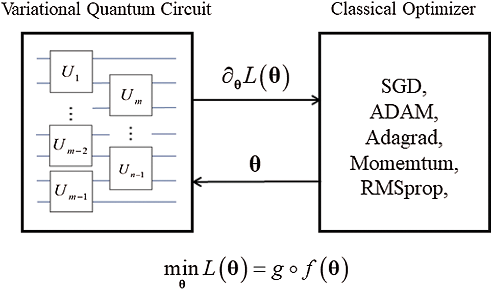
Figure 1: The framework of hybrid-based model

The works listed above form the problem as a non-convex optimization problem, such as minimizing or maximizing a composite function g∘f(θ), where f(θ) is the expectation value. The choice of function g can refer to the loss function in classical learning like mean square error (MSE), cross entropy loss etc.

f(θ)=〈O〉=tr(O⋅ρθ)(7)

where the observable O is the Hermitian operator of interest. In general, the density matrix ρθ can be described as an ensemble of pure states,

ρθ=∑j=1npj|φj〉〈φj|(8)

where ∑jpj=1. In the most of literatures, the pure state |φj〉 is produced by applying a variational quantum circuit U(θj) on initial quantum state |φ0〉, that is

|φj〉=U(θj)|φ0〉(9)

By virtue of the success of QAOA, the non-convex optimization of the loss function g∘f(θ) can also be optimized by gradient descent or heuristic algorithms.

Variational quantum circuit (VQC), known as the parametrized quantum circuit, plays the core role in the hybrid quantum-classical framework. It can be viewed as the quantum black-box model that is capable of approximating any given unitary operator with a small error like neural networks in classical machine learning [13]. Unlike neural networks using weight matrices (parameters) between layers that are adjusted by back-propagation methods, VQC achieves a similar work in the quantum setting by utilizing a sequence of fixed and parametrized quantum gates to construct a circuit model with a specific structure, that is

U(θ)=UθNUθN-1⋯Uθ2Uθ1(10)

where Uθj can be regarded as a quantum gate acting on specific qubits. They are selected from a gate set that consists of parameter-free quantum gates including Pauli matrices (σX, σY, σZ), controlled NOT gate (CNOT) and parametrized gates such as rotation gates (RX(θ), RY(θ), RZ(θ)). Besides, Uθj can also represent a quantum circuit block, a similar role of the layer in neural network, that is built by quantum gates with the specific structure. The widely used ways to construct variational quantum circuits by Uθj are shown in Fig. 2.

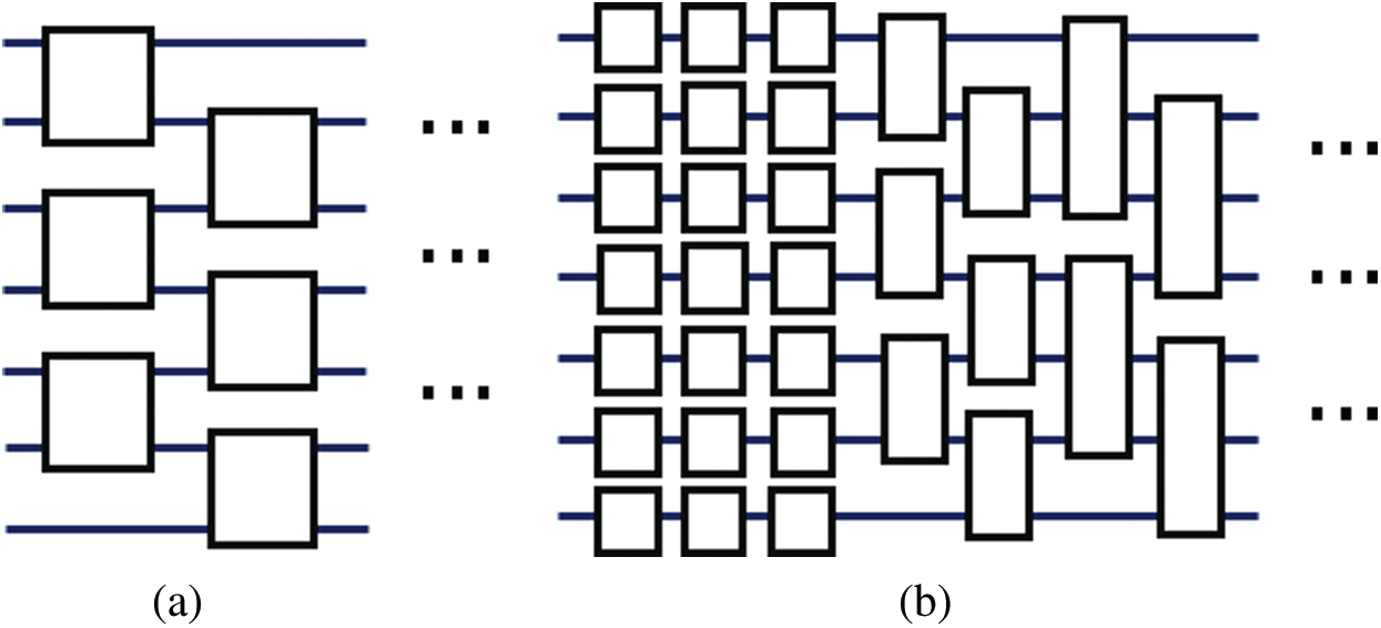
Figure 2: The structure of quantum circuit block Uθj. (a) Universal two-qubits gate, (b) one qubit gates+entanglement gates

In subgraph (a) of Fig. 2, each square represents the universal two-qubits gate which can be implemented by 15 rotation gates and 3 CNOT gates [27]. All these universal two-qubits gates are applied on nearest-neighbor qubits. If the size of the quantum system is n qubits and number of the layer is l, this type of structure requires 15(n-1)l quantum gates to create. In subgraph (b) of Fig. 2, the gates of Uθj is divided into two parts, the layer of one qubit gates and the layer of entangling gates. The squares represent the one rotation gates with angle and the rectangles stand for the entangling gates such as CNOT gates or Ising (XX, YY, ZZ) coupling gates. The details of these quantum gates are listed in Appendix A.

4  Learning Unitary by QML

Different from the methods introduced to solve the problem of learning a unitary transformation in Section 2, we reformulate the problem from another perspective. According to Choi–Jamiołkowski isomorphism in quantum information theory [11], there is the correspondence between a quantum mapping E and quantum states ρE such that,

ρE=E⊗I(ρΦ)=1d∑i,j=0d-1E(|i〉〈j|)⊗|i〉〈j|(11)

where ρE is known as Choi matrix which is identical to the quantum map E and ρΦ is the maximally entangled state,

ρΦ=1d∑i,j=0d-1|i,i〉〈j,j|(12)

Since the unitary transformation UT can be regarded as a mapping E from one density matrix to another one. Thus the learning unitary problem can be formed as the follow optimization problem, that is minimizing the distance between quantum state ρUT and ρUθ.

minθL(ρUT,ρUθ)(13)

where the quantum state ρUθ is

ρUθ=Uθ⊗I(ρΦ)=1d∑i,j=0d-1Uθ(|i〉〈j|)Uθ†⊗|i〉〈j|(14)

The learning problem of Eq. (13) stands for finding the unitary operator which minimizes the average output fidelity when feed the maximally mixed state as the input to Uθ and UT. Thus, it is necessary to add a regularization term to the problem Eq. (13), which also guarantees the distance between Uθ and UT are still small enough. Therefore, the learning unitary problem is shown as follow,

minθL(ρUT,ρUθ)+λ∥UT-Uθ∥p(15)

There are many choices for L(⋅,⋅) and ∥⋅∥p in problem Eq. (15). Since the bad selection of L(⋅,⋅) and ∥⋅∥p will affect the performance of the model, the appropriate choice of L(⋅,⋅) and ∥⋅∥p is required. We will introduce the measure of distance between quantum states and between operators.

Given two quantum state ρA and ρB, the commonly used measure of distance for how ‘close’ between the quantum states are shown as follows,

•      Trace distance:

LT(ρA,ρB)=12tr((ρA-ρB)†(ρA-ρB))=sup0≤P≤Itr(P(ρA-ρB))

It can be viewed as a generalization of the total variation distance on probability distribution that satisfies the symmetry and triangle inequality. It is also related to the maximum probability of distinguish different quantum state. The variational form of trace distance is shown in the second line of Eq. (16) [28].

•      Fidelity:

LF(ρA,ρB)=tr(ρA1/2ρBρA1/2)

Although the fidelity is not a metric, it has many good properties, such as it is invariant unitary transformation, the value of fidelity lies within 0 and 1. It also can be interpreted as the angle between states on a unit sphere. If ρA, ρB are pure state, the fidelity can reduced to the overlap (inner product) between states.

•      Quantum Optimal Transport Distance:

LOT(ρA,ρB)= minπtr(πC)s.t. trX(π)=ρA,trY(π)=ρB

It is the quantum extension of classical optimal transport distance [10]. However, it is semi-metric which does not satisfy the triangle inequality of metric on quantum states. It inherits the nice property of classical optimal transport distance including smoothness and continues.

Because the quantum optimal transport distance can naturally be implemented by hybrid quantum-classical framework on quantum device, we select quantum optimal transport distance as L(⋅,⋅).

Given a unitary operator U, the norm of operator U can be represented in a general form, namely Schatten p-norm, ∥U∥p=[tr(U†U)p/2]1/p.

•      Trace norm (p = 1):

∥U∥tr=∥U∥1=tr[(U†U)12]

•      The Frobenius norm (p = 2):

∥U∥F=∥U∥2=[tr(U†U)]12

•      The Spectral norm (p=∞):

∥U∥sp=∥U∥∞= max{∥Ux∥:x∈X,∥x∥=1}

where ∥⋅∥ is the Euclidean norm.

There are many nice properties of Schatten p-norm, such as the inequality between the different norms. For any operator X, if 1≤p≤q≤∞, then ∥X∥q≤∥X∥p [28]. Therefore, we have the following inequality between trace norm, Frobenius norm and spectral norm of operator X,

∥X∥sp≤∥X∥F≤∥X∥tr(16)

The related work employed the square of Frobenius norm as the loss function for learning unitary transformation [19]. In this work, we utilize the typically stronger norm, spectral norm, to estimate the error between approximate and desired unitary operator. Consequently, we can rewrite Eq. (15), the loss function of learning a unitary operator, in the following concrete way,

minθ,π maxu tr(πC)+λ∥UT-Uθ∥sps.t. trX(π)=ρUT,trY(π)=ρUθ(23)

Since the min-max problem of Eq. (23) can be considered as quantum GAN with regularization term. As directly solving the problem of Eq. (23) is intractable, we intend to tackle the dual form of this problem by the Lagrange multiplier technique.

minθmaxu,ϕ,φ tr(φ⋅ρUT)-tr(ϕ⋅ρUθ)+λ∥UT-Uθ∥sps.t.I⊗φ-ϕ⊗I≼C(24)

As the spectral norm of matrix A is to find the unit vector x which maximize the Euclidean norm of Ax, we use a full-connected neural network with soft-max layer to construct unit vector x, i.e., x=fsoftmax(W⋅x0+b). Moreover, we regard the variational quantum circuit Uθ as the generator and the parametrized observables φ,ϕ as the discriminator. On account of the variational quantum circuit can naturally be used for modeling the unitary transformation Uθ, we investigate the feasibility of applying the hybrid quantum classical framework to solve the optimization problem shown as Eq. (24). By applying the gradient based optimization algorithm, we iteratively adjust the parameters of quantum circuit to approximate the target unitary operator. Inspired by the training process of classical generative adversarial network, we also apply the strategy of alternately updating the parameters of generator and discriminator. The training algorithm is shown in Algorithm 1.

5  Experimental Results

In this section, we provide the experiments of applying the quantum machine learning model for learning the unitary transformation. We apply the quantum machine learning model discussed above to the task of learning the unitary transformation of one dimensional Heisenberg spin model which is also considered in reference [29]. The target unitary operator UT on N-qubit system is given by,

UT=e-i⋅H⋅t(25)

In which the Hamiltonian H is described as,

H=∑j=1Nσ⇀j⋅σ⇀j+1+hjσjz,σ⇀j=(σjx,σjy,σjz)(26)

where σ⇀j stands for a vector of Pauli matrices σx, σy, σz on jth qubit, and the external magnetic field hj in the z direction is randomly chosen from − h to h. We investigate the following cases that the system size N=2,3 and the evolution time t = N, and h = 1.

In Figs. 3 and 4, we provide the changes of trace norm, Frobenius norm and spectral norm between target and generated unitary operator during the training process. The solid black line represents the average norm for 10 runs with random initialization of parametrized quantum circuit, and the shaded area refers to the range of variation of the norm. In all case, the norm will approximate to zero which means the generated unitary operator is close to the target. In addition, the small system will lead to faster convergence, which is same as we expected.

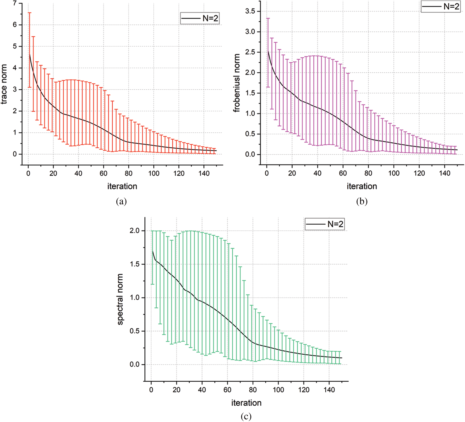
Figure 3: The trace norm, Frobenius norm and spectral norm vs. iterations (N=2). (a) Trace norm (N=2), (b) Frobenius norm (N=2), (c) spectral norm (N=2)

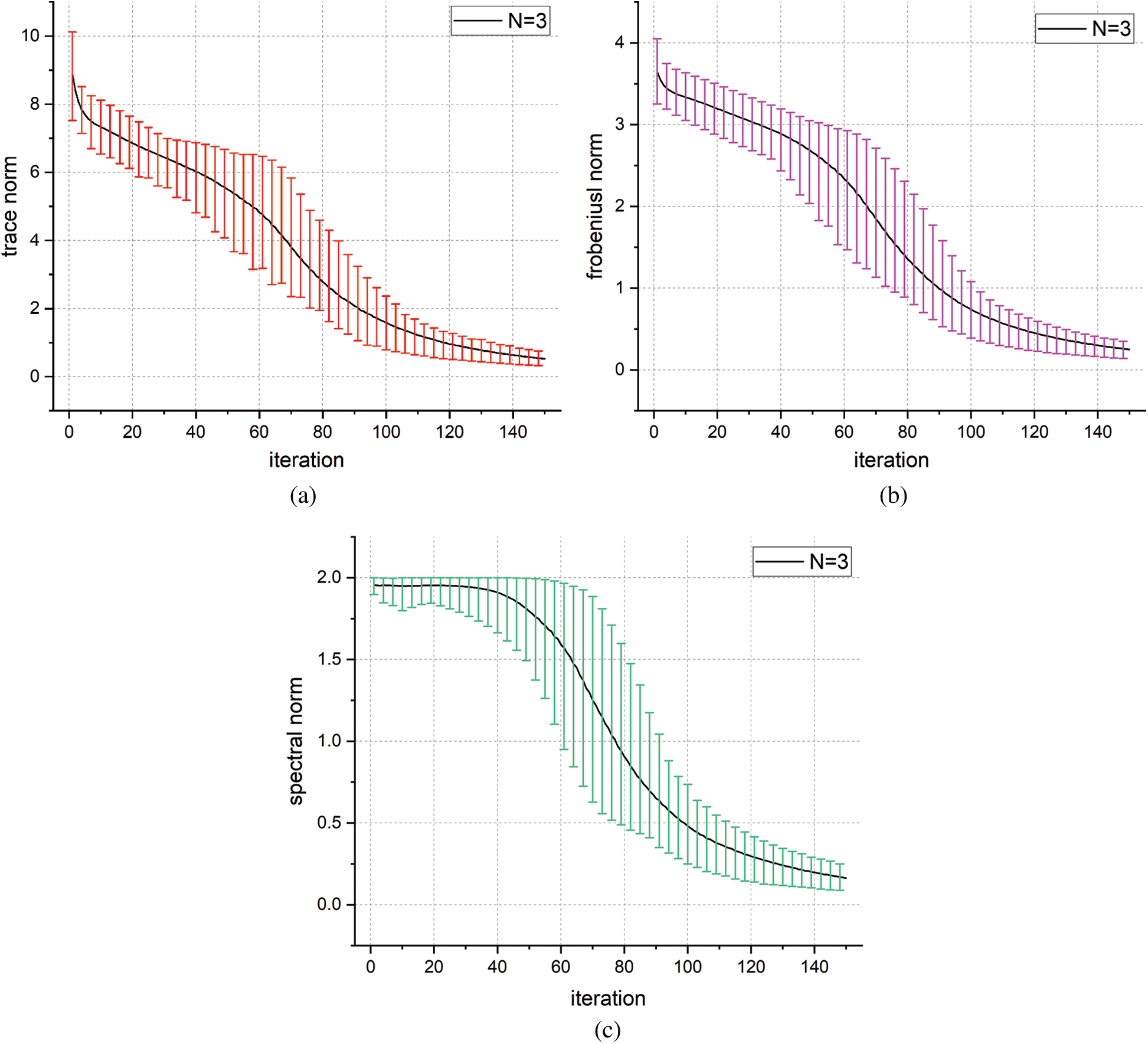
Figure 4: The trace norm, Frobenius norm and spectral norm vs. iterations (N=2). (a) Trace norm (N=2), (b) Frobenius norm (N=2), (c) spectral norm (N=2)

We select fidelity between the generated and target quantum states to evaluate the performance of our model. In Fig. 5, we show the fidelity between the quantum states which are generated by applying Uθ and UT on the same random input quantum states. As shown in Fig. 5, the fidelity is eventually around 0.997 which indicates that the generated quantum circuit provides a practicable approximation.

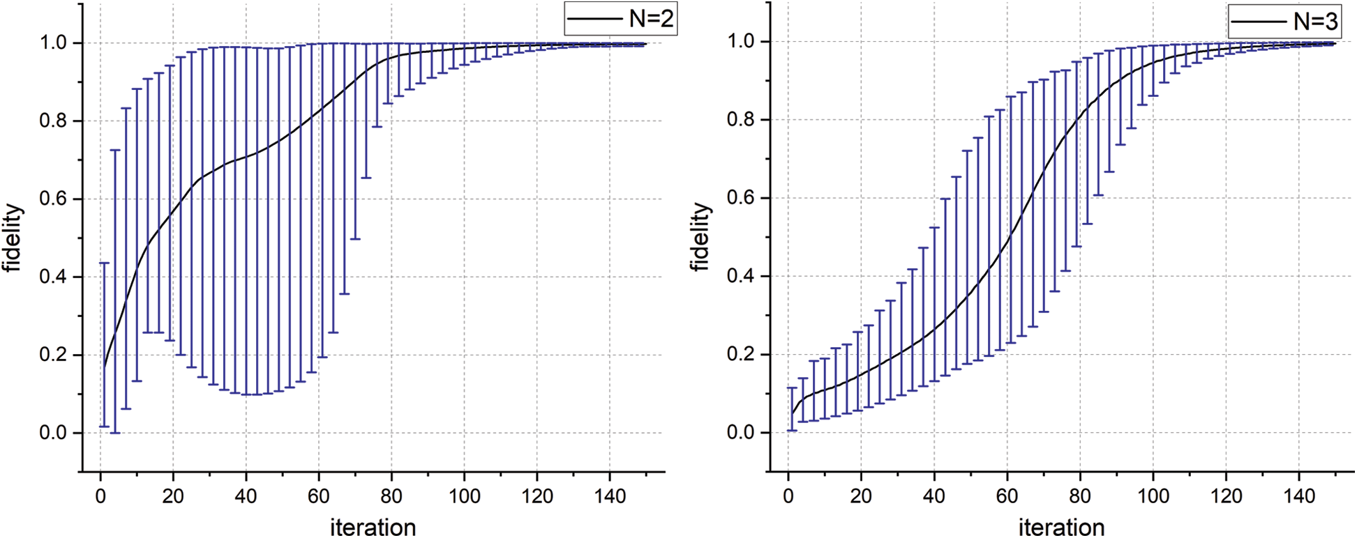
Figure 5: The fidelity of the states generated by applying U θ on random input (N=2, 3)

6  Discussion

Learning unitary transformation is an important and vexing task in quantum computing, which is related to controlling a quantum system or implementing a quantum algorithm with fewer resources. In this work, we investigate the use of promising techniques from quantum machine learning for learning a unitary transformation of a quantum system. Instead of the related works which formulate the learning problem as minimizing the norms between target and generated unitary operator, we express the problem as a quantum generative adversarial network with regularization term from the other perspective based on Choi–Jamiołkowski isomorphism. Comparing the trace norm and Frobenius norm used in related works, we add an intuitively stronger norm, spectral norm, as the regularization term to the loss function. Our numerical experiments demonstrate that the operator generated by our proposed model can successfully approximate the desired target unitary operator. The average spectral norm error of 10-replication runs is 0.1, and the average fidelity between the states produced by applying target and generated operators on the random input is around 0.997. Meanwhile, compared to the traditional method using product formulas for Hamiltonian simulation, our proposed model can significantly reduce the number of quantum gates for implementation. There are some potential applications of our proposed model such as providing help for assisting us in implementing quantum algorithms or compiling quantum circuits.

Acknowledgement: Thanks for constructive suggestion and helpful discussions from professor Xiaodi Wu.

Funding Statement: This work has received support from the National Key Research and Development Plan of China under Grant No. 2018YFA0306703.

Conflicts of Interest: The authors declare that they have no conflicts of interest to report regarding the present study.

Appendix A. Preliminary of Quantum Computing

A.1 Quantum State

Instead of storing a certain state in one classical bit, a qubit, the counterpart of classical bit, is in a superposition of two basic state |0〉 and |1〉. Let |φ〉 represents an arbitrary one-qubit state, which can be described by the |φ〉=α|0〉+β|1〉 or |φ〉=[αβ]T, where α and β are both complex number such that |α|2+|β|2=1. They are known as probability amplitude which means if we perform a measurement on state |φ〉, then |φ〉 will collapse into state |0〉 or state |1〉 with the probability |α|2 or |β|2, respectively. Besides, the quantum state |0〉 and |1〉 are also orthonormal bases, which are also called the computational bases in quantum computing. For a multi-qubit system, the state of this composite system can be described by the tensor product of the state of subsystem such as |φ〉=|φ1〉⊗⋯⊗|φm〉. All the quantum states we discussed above are pure states. Besides, a mixed state is an ensemble of some pure states {|φi〉} with coefficient pi, which is generally described by a density matrix in the form of ρ=∑ipi|φi〉〈φi|, and ∑ipi=1.

A.2 Quantum Gates and Quantum Circuit Model

The widely used model for quantum computation is the quantum circuit model that is constructed by a sequence of reversible quantum logic gates. In quantum mechanics, the time evolution of a quantum system can be described by a unitary transformation. Thus, the quantum logic gates are equivalent to the unitary transformations in the quantum circuit model. The followings are commonly used one-qubit and multiple-qubits quantum gates,

•      Puali Gates,

σx=[0110],σy=[0-ii0],σz=[100-1](A.1)

•      Rotation Gates,

Rx(θ)≡[cosθ/2-isinθ/2-i sin θ/2 cos θ/2],Ry(θ)≡[cosθ/2-isinθ/2 sin θ/2 cos θ/2],Rz(θ)≡[exp(-iθ/2)00 exp (iθ/2)](A.2)

•      Entangling Gates,

Controlled-NOT gate,

CNOT=[1000010000100001](A.3)

Ising XX Coupling Gates,

XX(ϕ)=[cosϕ00-isinϕ0cosϕ-isinϕ00isinϕcosϕ0-isinϕ00cosϕ](A.4)

An example of quantum circuit is shown in Fig. A.1, each solid line through quantum gates represents one qubit, which is corresponding to the passage of time. The square box denotes the quantum gates, i.e., the revolution of the quantum system. The quantum states are passed through the quantum gates from left to right.

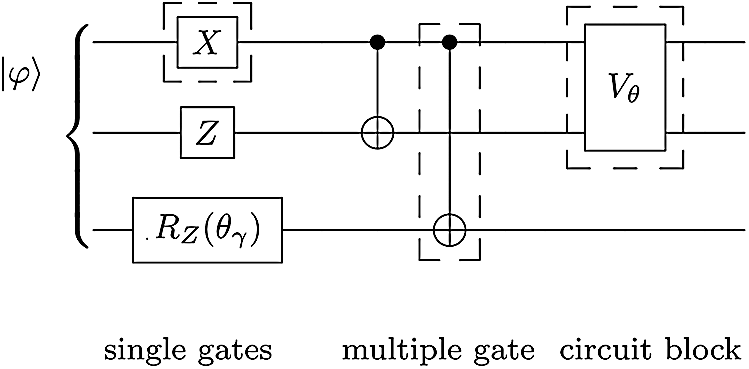
Figure A.1: An example of quantum circuit

A.3 Qubit Measurement

The classical data stored in quantum states cannot be directly read out. To extract the data, we have to perform the quantum measurement on the state. Due to the measurement involve the distraction from the exterior environment, the system will collapse after the measurement which is an irreversible action. The operation of measurement can be described by a group of measurement operator {Mi}, where ∑iMi†Mi=I. The projective measurement is simple and widely used measurement. It is described by an observable M which has the spectral decomposition, M=∑mm⋅Pm, where Pm=|ϕm〉〈ϕm| is the projector to the corresponding eigenspace with eigenvalue m. When we perform the projective measurement on state |φ〉, we can get the state |ϕm〉 with probability 〈ϕm|Pm|ϕm〉 and the expectation value E(M) of observable M, E(M)=tr(Mρ), where ρ is the density matrix of state |φ〉.

This work is licensed under a Creative Commons Attribution 4.0 International License, which permits unrestricted use, distribution, and reproduction in any medium, provided the original work is properly cited.