Computers, Materials & Continua DOI:10.32604/cmc.2021.016894
Article

Kernel Entropy Based Extended Kalman Filter for GPS Navigation Processing

Dah-Jing Jwo*and Jui-Tao Lee

Department of Communications, Navigation and Control Engineering, National Taiwan Ocean University, Keelung, 202301, Taiwan
*Corresponding Author: Dah-Jing Jwo. Email: djjwo@mail.ntou.edu.tw
Received: 12 January 2021; Accepted: 14 February 2021

Abstract: This paper investigates the kernel entropy based extended Kalman filter (EKF) as the navigation processor for the Global Navigation Satellite Systems (GNSS), such as the Global Positioning System (GPS). The algorithm is effective for dealing with non-Gaussian errors or heavy-tailed (or impulsive) interference errors, such as the multipath. The kernel minimum error entropy (MEE) and maximum correntropy criterion (MCC) based filtering for satellite navigation system is involved for dealing with non-Gaussian errors or heavy-tailed interference errors or outliers of the GPS. The standard EKF method is derived based on minimization of mean square error (MSE) and is optimal only under Gaussian assumption in case the system models are precisely established. The GPS navigation algorithm based on kernel entropy related principles, including the MEE criterion and the MCC will be performed, which is utilized not only for the time-varying adaptation but the outlier type of interference errors. The kernel entropy based design is a new approach using information from higher-order signal statistics. In information theoretic learning (ITL), the entropy principle based measure uses information from higher-order signal statistics and captures more statistical information as compared to MSE. To improve the performance under non-Gaussian environments, the proposed filter which adopts the MEE/MCC as the optimization criterion instead of using the minimum mean square error (MMSE) is utilized for mitigation of the heavy-tailed type of multipath errors. Performance assessment will be carried out to show the effectiveness of the proposed approach for positioning improvement in GPS navigation processing.

Keywords: GPS; satellite navigation; extended Kalman filter; entropy; correntropy; multipath; non-Gaussian

1  Introduction

Non-Gaussian noise is often encountered in many practical environments where the estimation performance deteriorates dramatically. Multipath [1] is known to be one of the dominant error sources in high accuracy global navigation satellite systems (GNSS) positioning systems, such as the Global Positioning System (GPS) [1,2]. Multipath effects occur when GPS signals arrive at a receiver site via multiple paths due to reflections from nearby objects, such as the ground and water surfaces, buildings, vehicles, hills, trees, etc. Many estimation algorithms have been studied to eliminate the positioning error caused by multipath. Since multipath errors are among uncorrelated errors that are not cancelled out during observation differencing, the performance of high precision GPS receivers are mostly limited by the multipath induced errors. One of the most important issues in GPS system performance improvement is the interference suppression techniques.

Due to its simple structure, stable performance and low computational complexity, the conventional adaptive filtering algorithm where the least mean square error (MSE) is involved has been widely used in a variety of applications in the fields of adaptive signal processing and machine learning. However, the MSE criterion is limited to the assumption of linearity and Gaussianity while most of the noise in real word is non-Gaussian. The performance deteriorates significantly in the non-Gaussian noise environment. The well-known Kalman filter (KF) [2,3] provides optimal (minimum MSE) estimate of the system state vector and has been recognized as one of the most powerful state estimation techniques. The traditional Kalman-type filter provides the best filter estimate when the noise is Gaussian, but most noise in real life is unknown, uncertain and non-Gaussian. Since the Kalman filter uses only second order signal information, it is not optimal when the system is disturbed by heavy-tailed (or impulsive) non-Gaussian noises. The extended Kalman filter (EKF) is a nonlinear version of the KF and has been widely employed as the GPS navigation processor. The fact that EKF highly depends on a predefined dynamics model forms a major drawback. To solve the performance degradation problem with non-Gaussian errors or heavy-tailed non-Gaussian noises, some robust Kalman filters have been developed by using non-minimum MSE criterion as the optimality criterion.

As a unified probabilistic measure of uncertainty quantification, entropy [4–6] has been widely used in information theory. The novel schemes using entropy principle based nonlinear filters are suitable as alternatives for GPS navigation processing. The robustness of algorithms has become a crucial issue when dealing with the practical GPS navigation application in non-Gaussian noise environments. In the cases where the additive noises in signal processing is supposed as Gaussian process, the MSE can be adopted for construction of the kernel adaptive filtering algorithms. The algorithm can suppress the effects of impulsive noise through kernel function in entropy, thus guarantees a good performance for non-Gaussian application. By introducing entropy/correntropy, kernel recursive algorithm based on minimum error entropy/maximum correntropy criterion can be employed to overcome the deteriorating performance where the LMS algorithm is involved for non-Gaussian signal. The minimum error entropy (MEE) criterion [7–9] and maximum correntropy criterion (MCC) [10–16] are information theoretic learning (ITL) approaches, which have been successfully applied in robust regression, classification, system identification and adaptive filtering. The algorithm updates equation recursively by minimizing the error entropy/maximizing the correntropy between output of the system and the desired signal. As compared with LMS, both the MEE and MCC algorithm possess better stability in non-Gaussian environments.

As a novel performance index, some of filters applied to non-Gaussian systems have been proposed. The MEE criterion is an important learning criterion in ITL, which has been successfully applied in robust regression, classification, system identification and adaptive filtering and has been widely adopted in non-Gaussian signal processing. The MEE scheme is designed by introducing an additional term, which and is tuned according to the higher order moment of the estimation error. The algorithm has a high accuracy in estimation because entropy can characterize all the randomness of the residual. The MEE adopted to minimize the error to obtain the maximum amount of information through measuring error information and ensures the local stability of the error dynamic. The MEE is a method of information theory learning which has been successfully applied to Kalman filters to improve robustness against pulsed noise. Information theory learning has been successfully applied to robust regression, classification, system recognition and adaptive filtering. The MCC is another important learning criterion which has been successfully used to handle the heavy-tailed non-Gaussian noise. Maximizing the mutual information between a state and the estimate is equivalent to minimizing the entropy of the estimation error. Based on information theory, another entropy criterion is proposed. Many experiments have shown that although MEE achieves excellent performance, the computational complexity is slightly higher than MCC.

The kernel entropy based EKF is adopted for the GPS navigation processing. Performance evaluation will be conducted to investigate the performance based on the two alternative entropy-related criteria: MEE and MCC. Results will be given to demonstrate the superiority of the designs with appropriate kernel bandwidth. Adaptive algorithms under MEE and MCC show enhanced robustness in the presence of non-Gaussian disturbances or heavy-tailed interference errors, such as the multipath interference. The remainder of this paper is organized as follows. In Section 2, preliminary background on the EKF and AEKF is reviewed. Section 3 addresses the basic principles on entropy theory, includes the MEE and MCC. The MEE- and MCC- based EKF’s are introduced in Section 4, where the MCC-based AEKF is also presented. In Section 5, numerical experiments are carried out to evaluate the performance using the proposed MCC-AEKF as compared to the other approaches. Conclusion is given in Section 6.

2  The Extended Kalman Filter and Covariance Scaling

Given a non-linear single model equation in discrete time

xk+1=f(xk)+wk (1)

zk=h(xk)+vk (2)

where the state vector xk∈ℜn, process noise vector wk∈ℜm, measurement vector zk∈ℜm, measurement noise vector vk∈ℜm, Qk is the process noise covariance matrix and Rk is the measurement noise covariance matrix.

The vectors wk and vk in Eqs. (1) and (2) are zero mean Gaussian white sequences has zero cross-correlation with each other:

E[wkwiT]=Qkδik;E[vkviT]=Rkδik;E[wkviT]=0forallkandi(3)

where E[⋅] represents expectation, and superscript “T” denotes matrix transpose. The symbol δik stands for the Kronecker delta function:

δik={1,i=k0,i≠k

The discrete-time adaptive extended Kalman filter algorithm is summarized as follow:

—Initialize state vector and state covariance matrix: x^0 and P0

Stage 1: correction steps/measurement update equations

(1) Compute Kalman gain matrix:

Kk=Pk∣k-1HkT[HkPk∣k-1HkT+Rk]-1(4)

(2) Update state vector:

x^k=x^k∣k-1+Kk[zk-h(x^k∣k-1)](5)

(3) Update error covariance

The error covariance relationships for a discrete filter with the same structure as the Kalman filter, but with an arbitrary gain matrix are written as

Pk=[I-KkHk]Pk∣k-1[I-KkHk]T+KkRkKkT(6)

Stage 2: Prediction steps/time update equations

(4) Predict state vector

x^k+1∣k=f(x^k)(7)

(5) Predict state covariance matrix

Pk+1∣k=ΦkPkΦkT+Qk(8)

where the linear approximation equations for system and measurement matrices are obtained through the relations

Φk≈∂f∂x|x=x^k∣k-1;Hk≈∂h∂x|x=x^k∣k-1

The discrete-time adaptive extended Kalman filter (AEKF) algorithm is summarized as follow.

(1) Compute measurement residual:

From the incoming measurement zk and the optimal prediction x^k∣k-1 obtained in the previous step, the innovations sequence is defined as υk=zk-h(x^k∣k-1). The innovation reflects the discrepancy between the predicted measurement h(x^k∣k-1) and the actual measurement zk. It represents the additional information available to the filter as a consequence of the new observation.

(2) The covariance of measurement residual matrix

By taking variances on both sides, we have the theoretical covariance, the covariance matrix of the innovation sequence is given by

Cυk=E[υkυkT]=HkPk∣k-1HkT+Rk(9)

(3) Estimate the innovation covariance

Defining C^υk as the statistical sample variance estimate of Cυk, matrix C^υk can be computed through averaging inside a moving estimation window of size N

C^υk=1N∑j=j0kυjυjT(10)

where N is the number of samples (usually called the window size); j0 = k − N + 1 is the first sample inside the estimation window. The window size N is chosen empirically (a good size for the moving window may vary from 10 to 30, and N=15 has been used in this paper) to give some statistical smoothing.

(4) Compute the forgetting factor

λk= max{1,trace[C^υk]trace[Cυk]}(11)

One of the other approaches for adaptive processing is on the incorporation of fading factors. The idea of fading memory is to apply a factor matrix to the predicted covariance matrix to deliberately increase the variance of the predicted state vector:

Pk+1∣k=λkΦkPkΦkT+Qk(12)

where λk=diag(λ1,λ2,…,λm). The main difference between different fading memory algorithms is on the calculation of scale factor matrix λk. One approach is to assign the scale factors as constants. When λi≤1 (i=1,2,…,m), the filtering is in a steady state processing while λi>1, the filtering may tend to be unstable. For the case λi=1, it deteriorates to the standard Kalman filter.

3  Entropy

From the definition of the information theoretic and kernel methods, entropy is a measure of the uncertainty associated with random variables. ITL is a framework to non-parametrically adapt systems based on entropy and divergence. Correntropy denotes a generalized similarity measure between two random variables.

3.1 Minimum Error Entropy

Originally presented by Shannon in 1948, many definitions of entropy have been introduced for various purposes, such as Shannon entropy and Renyi’s entropy. Renyi’s entropy, named after Alfred Renyi, is usually used for quantifying the diversity, uncertainty or randomness of a random variable. The quadratic Renyi’s entropy, which has the form

H2(X)=-log∫fX2(x)dx(13)

There are numerous methods to estimate the probability density. The kernel density estimation (KDE) has wide applicability and is closely related to the Renyi’s entropy. Kernel density estimation, also called Parzen window method, is a nonparametric method to estimate the probability density function of a random process. One can estimate the quadratic information potential of error entropy using a sample mean estimator as follow as

V^2(e)=1N∑i=1NGσ(ei)=1N2∑i=1N∑j=1Nκσ(ei-ej)(14)

where

kσ(x,y)=Gσ(ei)=12πσexp(-ei22σ2)(15)

denotes the Gaussian kernel, which is the most popular kernel function and is also adopted in this paper. Due to the negative logarithmic function monotonically decreasing function, it can be seen that minimizing the error entropy H2(e) means maximizing the information potential V^2(e).

3.2 Maximum Correntropy Criterion

In recent years, the maximum correntropy criterion has been successfully applied in many areas of signal processing, pattern recognition and machine learning with the existence of non-Gaussian noise, especially the large outliers.

Correntropy between two scalar variables measures the second-order information as well as higher-order statistical information in the joint probability density function. The correntropy of two random scalar variables X and Y is defined as

Vσ(X,Y)=E[κσ(X,Y)]=∫κσ(x,y)dFX,Y(x,y)=∫κσ(x,y)fXY(x,y)dxdy(16)

where E[⋅] represents the expectation operator, FX,Y(x,y) is the joint distribution, fXY(x,y) is the joint probability density function, and κσ(x,y) is a positive definite kernel function that satisfies the Mercer theory. In most practical situations, only limited amount of data is available and the joint distribution is usually unknown. In these cases, one can estimate the correntropy using a sample mean estimator as follow as

V^σ(X,Y)=1N∑i=1NGσ(ei)=1N∑i=1Nκσ(xi-yi)(17)

where ei = xi − yi, σ>0 denotes the kernel bandwidth. In most practical applications, the number of data we could access is scant and the joint distribution FX,Y(x,y) is usually unavailable. For solving this problem, one can use the sample mean square to estimate the correntropy. Taking the Taylor series expansion of the Gaussian kernel, we have

Vσ(X,Y)=∑n=0∞(-1)n2nσ2nn!E[(X-Y)2n](18)

It can been seen that correntropy represents a weighted sum of all even order moments of the two random variables X and Y. The kernel bandwidth appears as a parameter weighting the second order and higher order moments. With a very large (compared to the dynamic range of the data), the correntropy will be dominated by the second order moment, and then the maximum correntropy criterion will be approximately equal to the minimum mean square error criterion.

4  The Kernel Entropy Based Extended Kalman Filter

Consider an augmented model given by state prediction error with the measurement equation as

[x^k∣k-1zk]=[xkh(xk)]+[δxkvk](19)

where δxk is the state prediction error as δxk=x^k∣k-1-xk and we have

φk=[x^k∣k-1-xkvk](20)

The covariance matrix for φk can be represented by the joint matrix composed of Pk∣k-1 and Rk matrices, and Bk can be obtained by Cholesky decomposition of the joint matrix.

E[φkφkT]=BkBkT=[Pk∣k-100Rk]=[Bp,k∣k-1Bp,k∣k-1T00Br,kBr,kT]=[Bp,k∣k-100Br,k][Bp,k∣k-100Br,k]T(21)

Multiplying both sides on Eq. (19) by Bk-1, we have

εk=Dk-gk(xk)(22)

where

Dk=Bk-1[x^k∣k-1zk],gk(xk)=Bk-1[xkh(xk)],εk=Bk-1[δxkvk]=Bk-1φk(23)

E[εkεkT]=E[Bk-1φkφkT(Bk-1)T]=E[I]=I(24)

where I is denoted the n×n identity matrix, and the i-th row element in εk is

εi,k=di,k-gi,k(xk)(25)

4.1 Minimum Error Entropy-Based Extended Kalman Filter

The idea for the MEE-based EKF is to optimize the following cost function JMEE

JMEE(xk)=1L2∑i=1L∑j=1LGσ(εj,k-εi,k)(26)

Taking its derivative with respect to xk and setting it to zero

∂JMEE(xk)∂xk=0(27)

we have

x^k∣k= argmaxxkJMEE(xk)= argmaxxk∑i=1L∑j=1LGσ(εj,k-εi,k)(28)

The solution cannot be obtained in closed form even for a simple linear regression problem, so one has to solve it using an iterative update algorithm such as the gradient based methods. The gradient based methods are simple and widely used. However, they depend on a free parameter step-size and usually converge to an optimal solution slowly. The fixed-point iterative algorithm is an alternative efficient way to solve the solution, which involves no step-size and may converge to the solution very fast. The computation procedures for the minimum error entropy based extended Kalman filter (MEE-EKF) are summarized as follows:

1.    Choose a kernel bandwidth σ and the error tolerance ε with small positive value. Set the initial estimate and covariance x^0, P0;

2.    Perform Cholesky decomposition to obtain Bp,k∣k-1;

3.    Let x^k,0=x^k∣k-1, where x^k,t represents the state estimate at the fixed-point iteration t;

4.    Iteration loop: Calculation of x^k,t using the following steps:

5.    ẽi,k=di,k-gi,k(x^k,t)

6.    [Φk]ij=Gσ(εj,k-εi,k)

7.    Ψk=diag{∑i=1LGσ(ε1,k-εi,k),…,∑i=1LGσ(εL,k-εi,k)}

8.    C̃k=Φk-Ψk=[C̃x,kC̃zx,kC̃xz,kC̃z,k]

9.    P̃xx,k∣k-1=(Bp,k∣k-1-1)TC̃x,kBp,k∣k-1-1

10.   P̃xz,k∣k-1=(Bp,k∣k-1-1)TC̃xz,kBr,k-1

11.   P̃zx,k∣k-1=(Br,k-1)TC̃zx,kBp,k∣k-1-1

12.   R̃k=(Br,k-1)TC̃z,kBr,k-1

13.   K̃k=(P̃xx,k∣k-1+HkTP̃xz,k∣k-1+(P̃zx,k∣k-1+HkTR̃k)Hk)-1(P̃zx,k∣k-1+HkTR̃k)

x^k,t=x^k∣k-1+K̃k[zk-hk(x^k∣k-1)]

Compare the estimation for the current steps with the previous steps for convergence check

∥x^k,t-x^k,t-1∥∥x^k,t-1∥≤ε

If the above condition holds, then set x^k=x^k,t, go to Step 6, otherwise, go back to Step 4

Calculation of update covariance matrix:

Pk=(I-K̃kHk)Pk∣k-1(I-K̃kHk)T+K̃kRkK̃kT

Predict x^k+1∣k and Pk+1∣k. Set k+1→k, and go back to Step 2

x^k+1∣k=f(x^k)Pk+1∣k=ΦkPkΦkT+Qk

4.2 Maximum Correntropy Criterion-Based Extended Kalman Filter

The idea to optimize the following cost function JMCC

JMCC(xk)=∑i=1LGσ(di,k-gi,k(xk))(29)

can be obtained by solving

∂JMCC(xk)∂xk=0(30)

and we have

xk∣k= argmaxxkJMCC(xk)= argmaxxk∑i=1LGσ(di,k-gi,k(xk))= argmaxxk∑i=1LGσ(ei,k)(31)

The covariance matrices Pk∣k-1 and Rk can be further expressed as

[Pk∣k-100Rk]=[Bp,k∣k-100Br,k][Cx,k00Cz,k]-1[Bp,k∣k-100Br,k]T=[Bp,k∣k-1Cx,k-1Bp,k∣k-1T00Br,kCz,k-1Br,kT](32)

where we have

Pk∣k-1=Bp,k∣k-1Cx,k-1Bp,k∣k-1T (33)

Rk=Br,kCz,k-1Br,kT (34)

The computation procedures for the maximum correntropy criterion based extended Kalman filter (MCC-EKF) are summarized as follows:

1.    Choose a kernel bandwidth σ and the error tolerance ε with small positive value. Set the initial estimate and covariance x^0, P0;

2.    Perform Cholesky decomposition to obtain Bp,k∣k-1;

3.    Let x^k,0=x^k∣k-1, where x^k,t represents the state estimate at the fixed-point iteration t;

4.    Iteration loop: Calculation of x^k,t using the following steps:

5.    ẽi,k=di,k-gi,k(x^k,t)

6.    C̃x,k=diag(Gσ(ẽ1,k),…,Gσ(ẽn,k))

7.    C̃z,k=diag(Gσ(ẽn+1,k),…,Gσ(ẽn+m,k))

8.    P̃k∣k-1=Bp,k∣k-1C̃x,k-1Bp,k∣k-1T

9.    R̃k=Br,kC̃z,k-1Br,kT

10.   K̃k=P̃k∣k-1HkT[HkP̃k∣k-1HkT+R̃k]-1

x^k,t=x^k∣k-1+K̃k[zk-hk(x^k∣k-1)]

Compare the estimation for the current steps with the previous steps for convergence check

∥x^k,t-x^k,t-1∥∥x^k,t-1∥≤ε

If the above condition holds, then set x^k=x^k,t, go to Step 6, otherwise, go back to Step 4

Calculation of update covariance matrix:

Pk=(I-K̃kHk)Pk∣k-1(I-K̃kHk)T+K̃kRkK̃kT

Predict x^k+1∣k and Pk+1∣k. Set k+1→k, and go back to Step 2

x^k+1∣k=f(x^k)Pk+1∣k=ΦkPkΦkT+Qk

4.3 Maximum Correntropy Criterion-Based Adaptive Extended Kalman Filter

Utilization of the MCC-AEKF is a treatment for further performance enhancement. Fig. 1 provides the flow chart for one cycle of the maximum correntropy criterion-based adaptive extended Kalman filter (MCC-AEKF), which involves the computation procedure in both MCC and AEKF.

To fulfil the requirement, an adaptive Kalman filter can be utilized as the noise-adaptive filter to estimate the noise covariance matrices and overcome the deficiency of Kalman filter. The benefit of the adaptive algorithm is that it keeps the covariance consistent with the real performance. The innovation sequences have been utilized by the correlation and covariance-matching techniques to estimate the noise covariances. The basic idea behind the covariance-matching approach is to make the actual value of the covariance of the residual consistent with its theoretical value.

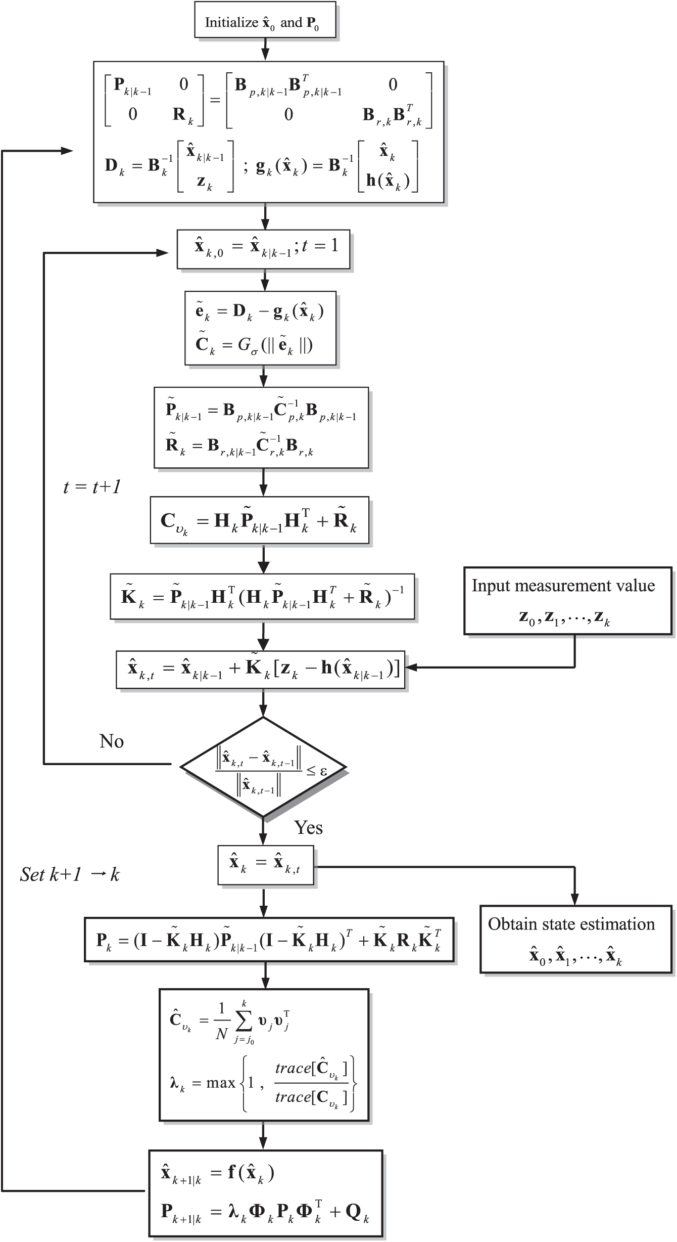
Figure 1: Flow chart for on cycle of the maximum correntropy criterion-based adaptive extended Kalman filter (MCC-AEKF)

5  Results and Discussion

To validate the effectiveness of the proposed approaches, simulation experiments have been carried out to evaluate the performance of the proposed kernel entropy based approach in comparison with the other conventional methods for GPS navigation processing. The kernel entropy principle assisted EKF for GPS navigation processing is presented. Two scenarios dealing with two types of interferences are carried out, including pseudorange observable errors involving (1) time-varying variance in the measurement noise, and (2) outlier type of multipath interferences, during the vehicle moving.

The computer codes were developed by the authors using the Matlab® software. The commercial software Satellite Navigation (SATNAV) Toolbox by GPSoft LLC [17] was employed for generation of the GPS satellite orbits/positions and thereafter, the satellite pseudoranges, carrier phase measurement, and constellation, required for simulation. The simulated pseudorange error sources corrupting GPS measurements include ionospheric delay, tropospheric delay, receiver noise and multipath. Assume that the differential GPS (DGPS) mode is available and therefore most of the receiver-independent common errors can be corrected, while the multipath and receiver thermal noise cannot be eliminated. The multipath interferences are added into the GPS pseudorange observation data during the vehicle moving. Since the research focus on the mitigation of multipath errors, the influence of measurement noise is relatively critical.

In the simulation, there are 9 GPS satellites available. The test trajectory for the simulated vehicle and the skyplot during the simulation time interval are shown as in Fig. 2. A vehicle is designed to perform the uniform accelerated motion to reduce the impact caused by unmodeling system dynamic errors. Performance comparison presented will cover two parts for each of the scenarios. Firstly, performance comparison for EKF, MEE-EKF and MCC-EKF is shown. Secondly, performance enhancement using covariance scaling is presented, where various types of approaches including EKF, AEKF MCC-EKF and MCC-AEKF are involved.

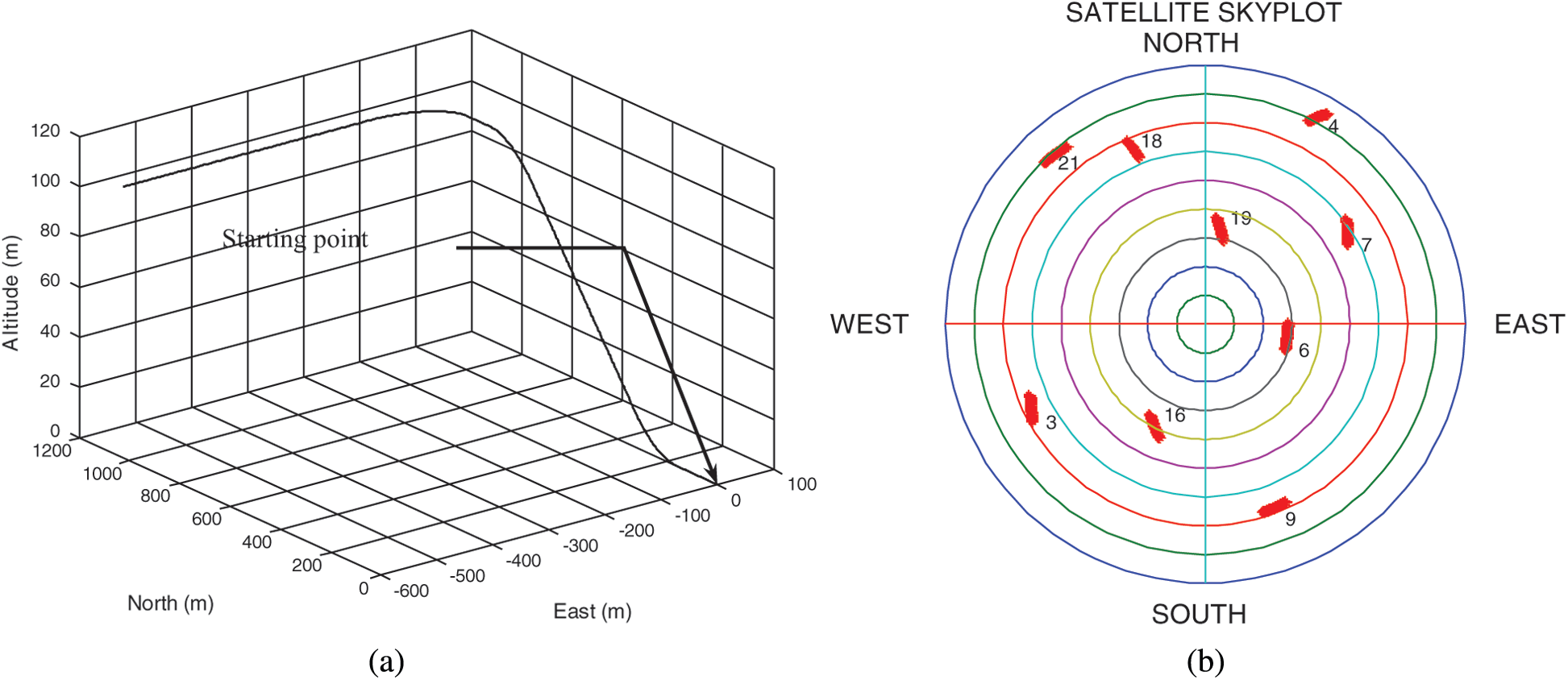
Figure 2: (a) Test trajectory for the simulated vehicle; and (b) the skyplot during the simulation

Table 1: Description of the time-varying noise strength in the five time intervals for Scenario 1

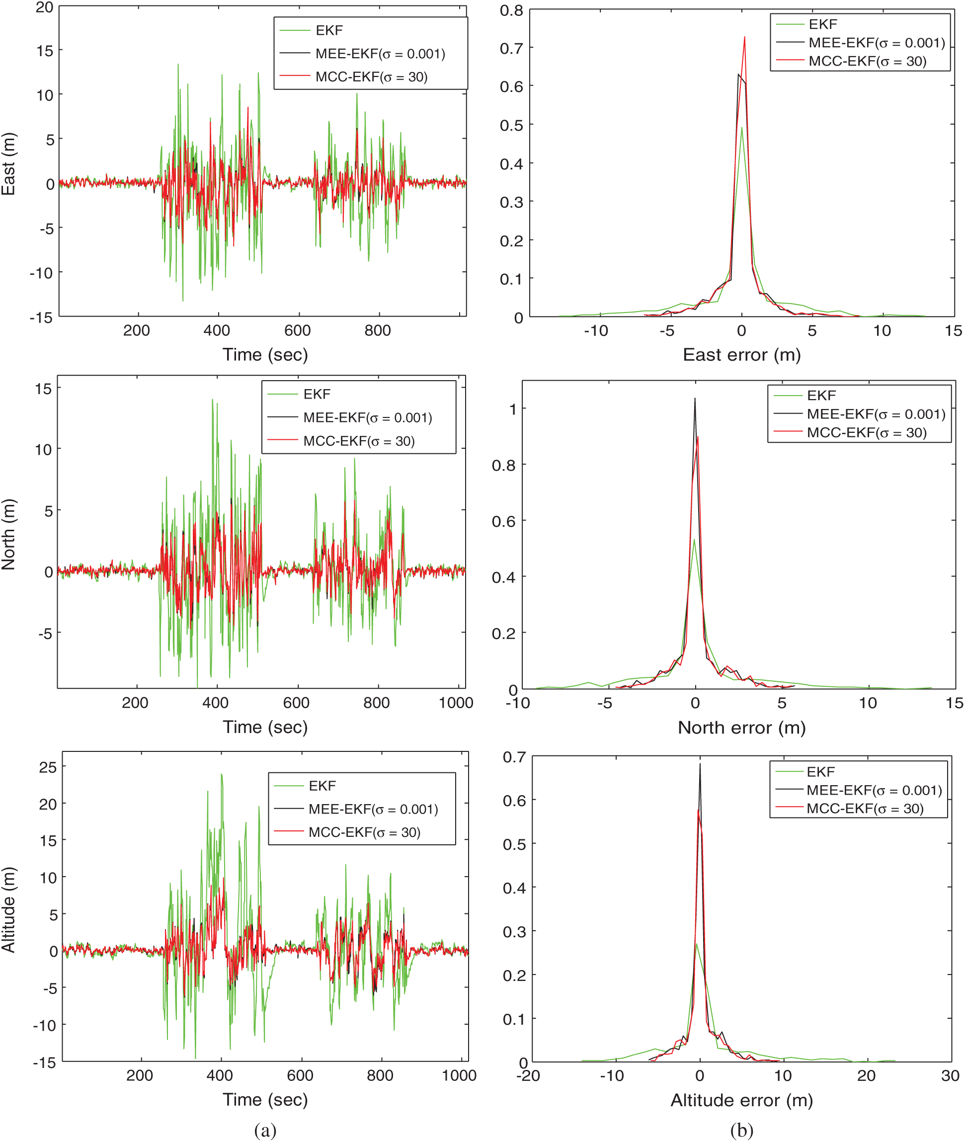
Figure 3: (a) Comparison of positioning accuracy and (b) the corresponding error probability density functions (pdf’s) for EKF, MEE-EKF and MCC-EKF—Scenario 1. (a) Position errors, (b) probability density functions

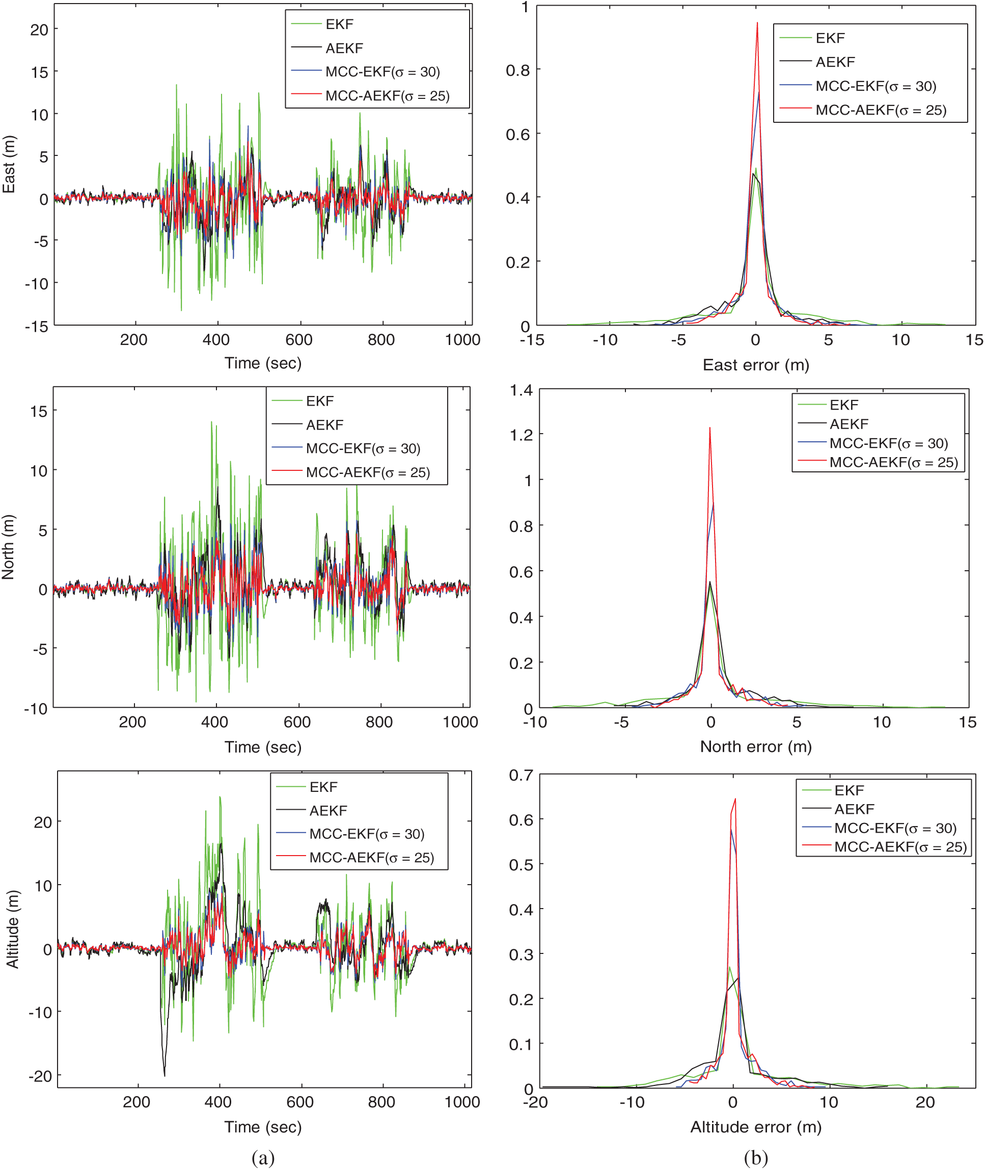
Figure 4: (a) Comparison of positioning accuracy and (b) the corresponding error pdf’s for EKF, AEKF MCC-EKF and MCC-AEKF—Scenario 1. (a) Position errors, (b) probability density functions

5.1 Scenario 1: Environment Involving Time-Varying Variance in Measurement Noise

Scenario 1 is designed for investigating the performance comparison when dealing with the time-varying measurement noise statistics. Description of time varying measurement variances in the five time intervals is shown in Tab. 1. The time-varying measurement noise variances rρi in the five time intervals for this scenario are assumed to follows the variation: rρi=1→16→1→10→1 (in unit of m2), where the ‘arrows (→)’ is employed for indicating the time-varying trajectory of variances. The set of unknown time-varying statistical parameters of noise needs to be estimated with the system state and the error covariance.

5.1.1 Performance Comparison for EKF, MEE-EKF and MCC-EKF

Comparison of GPS navigation accuracy for the EKF, MEE-EKF and MCC-EKF is shown in Fig. 3 where the positioning accuracy comparison and the corresponding error pdf’s, respectively, are shown. The results show that both MEE and MCC based EKF can effectively improve the positioning performance. As can be seen, both the MEE and MCC can be adopted to assist the EKF to improve GPS navigation accuracy in time-varying Gaussian noise environment where the filtering performance based on the two optimization criterion lead to equivalent results with no noticeable distinction.

5.1.2 Performance Enhancement Using Covariance Scaling

Comparison of positioning accuracy for the four algorithms: EKF, AEKF, MCC-EKF and MCC-AEKF is shown in Fig. 4, where both the positioning accuracy and the corresponding error pdf’s are presented. Fig. 5 shows the variation and adaptation capability of the standard deviation for the time-varying statistics in the measurement model. The MCC-EKF did not catch the variation of noise strength very well. With the assistance of AEKF, the MCC-AEKF can further improve the performance. From the other view point, the adaptation capability of noise variance for the AEKF has been improved with the assistance of the MCC mechanism. Tab. 2 provides the performance comparison for various algorithms. As compared MEE, the MCC based approach provides similar positioning accuracy with better computation efficiency. Of the various approaches, the MCC-AEKF provides the best positioning accuracy with only a little more execution time as compared to MCC-EKF.

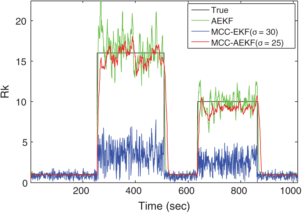
Figure 5: Variation and adaptation results of the variance for the time-varying measurement noise

Table 2: Performance comparison for various algorithms—Scenario 1

5.2 Scenario 2: Pseudorange Observable Involving Outlier Type of Multipath Errors

In Scenario 2, mitigation of the pseudorange observable involving outlier type of multipath interferences is discussed. There are totally five time durations where additional randomly generated errors are intentionally injected into the GPS pseudorange observation data during the vehicle moving. Tab. 3 shows the information of the outliers, including the numbers of outliers and their strengths.

Table 3: Information for the outliers

5.2.1 Performance Comparison for EKF, MEE-EKF and MCC-EKF

Comparison of GPS navigation accuracy for the three schemes: EKF, MEE-EKF and MCC-EKF is shown in Fig. 6 where both the comparison of positioning accuracy and the error corresponding pdf’s are presented. The results show that the both the MEE and MCC can assist EKF to effectively deal with the outliers in the pesudorange observables such as multipath interferences.

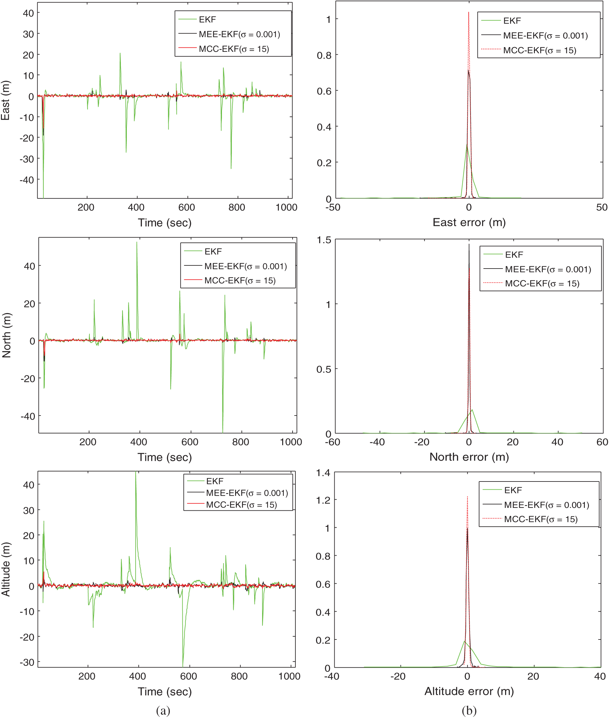
Figure 6: (a) Comparison of positioning accuracy and (b) the corresponding error pdf’s for EKF, MEE-EKF and MCC-EKF—Scenario 2. (a) Position errors, (b) probability density functions

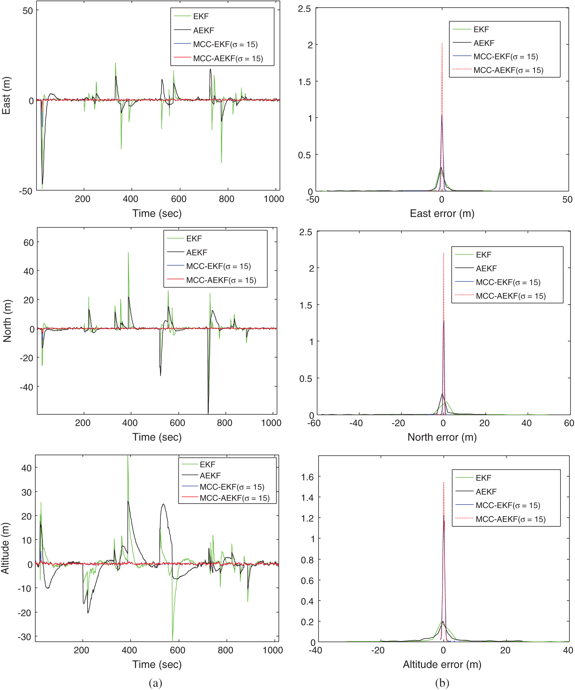
Figure 7: (a) Positioning accuracy comparison and (b) the corresponding error pdf’s for EKF, AEKF, MCC-EKF and MCC-AEKF—Scenario 2. (a) Position errors, (b) probability density functions

5.2.2 Performance Enhancement Using Covariance Scaling

Utilization of the AEKF, referred to as the MCC-AEKF, is employed for further performance enhancement. Fig. 7 illustrates the positioning accuracy and the corresponding pdf’s for various algorithms: EKF, AEKF, MCC-EKF and MCC-AEKF. The AEKF does not possess sufficient capability to resolve the outlier type of interference, while the MCC-AEKF demonstrates substantial performance improvement in navigation accuracy with acceptable extra computational expense. Tab. 4 summarizes the estimation performance and execution time for various algorithms.

Table 4: Performance comparison for various algorithms—Scenario 2

6  Conclusions

This paper investigates the kernel entropy principle based adaptive filtering for Global Positioning System (GPS) navigation processing. The algorithm is effective for dealing with non-Gaussian or heavy-tailed errors, such as the multipath interferences.

The standard EKF method is derived based on MSE criterion and is limited to the assumption of linearity and Gaussianity to be optimal. The robustness of nonlinear filter is improved using the optimization criterion based on entropy or correntropy. The GPS navigation algorithm based on kernel entropy related principles, including the MEE criterion and the MCC has been performed, which is especially useful for the heavy-tailed/impulsive types of interference errors. In addition, behavior of the innovation related parameters have been introduced, which are useful in designing the adaptive Kalman filter to form the MCC-AEKF for further performance improvement.

Simulation experiments for GPS navigation have been provided to illustrate the performance. Results show that the kernel entropy principle based adaptive filtering algorithm possesses noticeable improvement on navigation accuracy as compared to that of conventional methods and thus demonstrates good potential as the alternative as the GPS navigation processor, especially in the case of observables with non-Gaussian errors. Two scenarios, including (1) the environment involving time-varying measurement noise variance; and (2) the pseudorange observable involving outlier type of multipath errors, respectively, are presented for demonstration. Performance comparison for various approaches, including EKF, AEKF, MCC-EKF, MEE-EKF and MCC-AEKF have been carried out and the kernel entropy based EKF algorithm has demonstrated promising results in navigational accuracy improvement.

Funding Statement: This work has been partially supported by the Ministry of Science and Technology, Taiwan (Grant Number MOST 108-2221-E-019-013).

Conflicts of Interest: The authors declare that they have no conflicts of interest to report regarding the present study.

References

 1.  E. D. Kaplan and C. J. Hegarty. (2006). Understanding GPS: Principles and Applications, Norwood, MA, USA: Artech House, Inc. [Google Scholar]

 2.  R. G. Brown and P. Y. C. Hwang. (1997). Introduction to Random Signals and Applied Kalman Filtering, New York, NY, USA: John Wiley & Sons. [Google Scholar]

 3.  A. H. Mohamed and K. P. Schwarz. (1999). “Adaptive kalman filtering for INS/GPS,” Journal of Geodesy, vol. 73, pp. 193–203. [Google Scholar]

 4.  M. A. El-Sayed, A. A. Ali, M. E. Hussien and H. A. Sennary. (2020). “A multi-level threshold method for edge detection and segmentation based on entropy,” Computers, Materials & Continua, vol. 63, no. 1, pp. 1–16. [Google Scholar]

 5.  W. Liu, J. C. Principe and S. Haykin. (2010). Kernel Adaptive Filtering: A Comprehensive Introduction, Hoboken, NJ, USA: John Wiley & Sons. [Google Scholar]

 6.  J. C. Principe. (2010). Information Theoretic Learning, Renyi’s Entropy and Kernel Perspectives, New York, NY, USA: Springer. [Google Scholar]

 7.  B. Chen, L. Dang, Y. Gu, N. Zheng and J. C. Principe. (2019). “Minimum error entropy Kalman filter,” IEEE Transactions on Systems, Man, and Cybernetics: Systems, pp. 1–11, (Early Access). [Google Scholar]

 8.  B. Chen, Z. J. Yuan, N. N. Zheng and J. C. Principe. (2013). “Kernel minimum error entropy algorithm,” Neurocomputing, vol. 121, pp. 160–169. [Google Scholar]

 9.  M. Ren, J. Zhang, F. Fang, G. Hou and J. Xu. (2013). “Improved minimum entropy filtering for continuous nonlinear non-Gaussian systems using a generalized density evolution equation,” Entropy, vol. 15, no. 7, pp. 2510–2523. [Google Scholar]

10. B. Chen, X. Liu, H. Zhao and J. C. Principe. (2017). “Maximum correntropy Kalman filter,” Automatica, vol. 76, pp. 70–77. [Google Scholar]

11. B. Chen and J. C. Principe. (2012). “Maximum correntropy estimation is a smoothed MAP estimation,” IEEE Signal Processing Letters, vol. 19, no. 8, pp. 491–494. [Google Scholar]

12. B. Chen, L. Xing, J. Liang, N. Zheng and J. C. Principe. (2014). “Steady-state mean-square error analysis for adaptive filtering under the maximum correntropy criterion,” IEEE Signal Processing Letters, vol. 21, no. 7, pp. 880–884. [Google Scholar]

13. W. Liu, P. P. Pokharel and J. C. Principe. (2007). “Correntropy: Properties and applications in non-Gaussian signal processing,” IEEE Transactions on Signal Processing, vol. 55, no. 11, pp. 5286–5298. [Google Scholar]

14. X. Liu, H. Qu, H. Zhao and B. Chen. (2016). “Extended Kalman filter under maximum correntropy criterion,” in Proc. IEEE Int. Joint Conf. on Neural Networks, Vancouver, BC, Canada, pp. 1733–1737. [Google Scholar]

15. A. Singh and J. C. Principe. (2009). “Using correntropy as a cost function in linear adaptive filters,” in Proc. IEEE Proc. of the Int. Joint Conf. on Neural Networks, Atlanta, GA, USA, pp. 2950–2955. [Google Scholar]

16. S. Zhao, B. Chen and J. C. Principe. (2011). “Kernel adaptive filtering with maximum correntropy criterion,” in Proc. IEEE Proc. of the Int. Joint Conf. on Neural Networks, San Jose, CA, USA, pp. 2012–2017. [Google Scholar]

17. GPSoft LLC., Satellite Navigation Toolbox 3.0 User’s Guide, Athens, OH, USA. [Google Scholar]

This work is licensed under a Creative Commons Attribution 4.0 International License, which permits unrestricted use, distribution, and reproduction in any medium, provided the original work is properly cited.