[BACK]
Computers, Materials & Continua
DOI:10.32604/cmc.2021.012586 |  |
| Article | |
Wave Propagation Model in a Human Long Poroelastic Bone under Effect of Magnetic Field and Rotation
A. M. Abd-Alla1,*, Hanaa Abu-Zinadah2, S. M. Abo-Dahab3, J. Bouslimi4,5 and M. Omri6
1Department of Mathematics, Sohag University, Sohag, Egypt
2Department of Statistics, University of Jeddah, College of Science, Jeddah, Saudi Arabia
3Department of Mathematics, South Valley University, Qena, 83523, Egypt
4Department of Engineering Physics and Instrumentation,National Institute of Applied Sciences and Technology, Carthage University, Tunisia
5Department of Physics, Taif University, Taif, Saudi Arabia
6Deanship of Scientific Research, King Abdulaziz University, Jeddah, Saudi Arabia
*Correspondence: A. M. Abd-Alla. Email: mohmrr@yahoo.com
Received: 10 June 2020; Accepted: 20 August 2020
Abstract: This article is aimed at describing the way rotation and magnetic field affect the propagation of waves in an infinite poroelastic cylindrical bone. It offers a solution with an exact closed form. The authors got and examined numerically the general frequency equation for poroelastic bone. Moreover, they calculated the frequencies of poroelastic bone for different values of the magnetic field and rotation. Unlike the results of previous studies, the authors noticed little frequency dispersion in the wet bone. The proposed model will be applicable to wide-range parametric projects of bone mechanical response. Examining the vibration of surface waves in rotating cylindrical, long human bones under the magnetic field can have an impact. The findings of the study are offered in graphs. Then, a comparison with the results of the literature is conducted to show the effect of rotation and magnetic field on the wave propagation phenomenon. It is worth noting that the results of the study highly match those of the literature.
Keywords: Propagation of waves; rotation; magnetic field; poroelastic; wet bone; natural frequency; magnetic field
1 Introduction
One of the highly considerable clinical methods for identifying the integrity of bones in vivo is radiographic examination, though, X-ray cannot detect when the loss of a bone decreases less than 30%. By the same token, periodic X-rays can always be utilized in monitoring the healing of fractures although evaluating the healing degree is subjective and often inaccurate. Natall et al. [1] examined bones as a material from a biomechanical perspective. The authors of [2–7] explored various issues related to the propagation of waves within poroelastic cylinders. In regard to a porous anisotropic solid, Biot [8] introduced the theory of elasticity and consolidation. In another study, Biot [9] discussed the theory of elastic wave propagation in a solid that is fluid-saturated and porous. Cardoso et al. [10] investigated the role of the biological tissue structural anisotropy in the poroelastic propagation of waves. The authors of [11] solved issues related to the propagation of coupled poroelastic/acoustic/elastic waves through automatic hp-adaptively. In 3D poroelastic solids, Wen [12] used the meshless local Petrov–Galerkin method for the propagation of waves. Morin et al. [13] investigated the arduous multiscale poromicrodynamics method that is effective in the diverse bone tissues. Employing an iterative active medium approximation, Potsika et al. [14] introduced the model ultrasound propagation of waves in the healing of long bones. The authors of [15] analyzed theoretically the process of internal bone restoration motivated by a medullary pin. Nguyen et al. [16] investigated the performance of the flows of interstitial fluid in cortical bones controlled by axial cyclic harmonic loads that mimic the behavior of in vivo bones while doing daily activities, such as going for a walk. Misra et al. [17] derived the relation of dispersion for axisymmetric acoustic wave propagation along a long composite bone. Qin et al. [18] predicted theoretically the remodeling of the surface bone in the diaphysis of the long bone under different external loads controlled by the theory of adaptive elasticity. Mathieu et al. [19] studied biomechanically the performance of the bone-dental implant interface as an environmental task by taking into account the in silico, in vivo, and ex vivo projects on animal models. Brynk et al. [20] evaluated relevant experimental findings within a microporomechanic theoretical framework. Parnell et al. [21] compared the theoretical estimates of the active elastic moduli of cortical bone at the meso- and macroscales. Shah [22] studied the near-surface condition of stress established under the oscillatory contact between the artificial components that have a considerable role in defining fretting severity. Gilbert et al. [23] investigated the viscous interstitial fluid that plays a role in the ultrasound insonification of non-defatted cancellous bone. The authors of [24] solved analytically the noticeably long borehole in the isotropic and poroelastic medium inclined to the far-field principal stresses. Cowin [25] developed the interaction model of fluid and solid stages of a fluid-saturated porous medium. The effectiveness of bone healing in the ultrasonic reaction of the titanium implants that take the shape of coins and inserted in rabbit tibiae was discussed by Mathieu et al [26]. Singhal et al. [27] investigated the interior restoration of bone by defining the process that enables the bones to have the histological structure to modify within areas of long mechanical load. Kumha [28] investigated the shear wave in a primarily stressed poroelastic medium that has corrugated boundary surfaces inserted between a higher material strengthened with fiber and isotropic inhomogeneous half-space.
Abo-Dahab et al. [29] investigated the analytical solution for surface waves’ remodeling in the long bones under the magnetic field and rotating. Farhan [30] discussed the effect of rotation on the propagation of waves in a hollow poroelastic circular cylinder with a magnetic field. Marin et al. [31] investigated the structural continuous dependence in micropolar porous bodies. Abo-Dahab et al. [32] discussed the effect of rotation on the propagation of waves model in a human long poroelastic bone.
In this paper, the way rotation and magnetic field affect the propagation of waves in an infinite poroelastic cylindrical bone is discussed. The paper provides a solution with an exact closed form. The authors got and examined numerically the general frequency equation of the poroelastic bone. Moreover, they calculated the frequencies of the poroelastic bone for different values of the magnetic field and rotation. Unlike the results of the previous studies, the authors noticed little frequency dispersion in the wet bone. The proposed model will be applicable to wide-range parametric projects of bone mechanical response. Examining the vibration of surface waves in rotating cylindrical, long human bones under the magnetic field can have an impact. The findings of the study are offered in graphs. Then, a comparison with the results of the literature is conducted. It is worth noting that the results of the study highly match those of the literature.
2 Formulation of the Problem
Take into account a hollow cylinder in the form of a geometric approximation to a long bone that is well-defined in the cylindrical coordinates r,θ,z. To carry out the analysis, assume the z -axis as the long bone axis and a and b as the internal and external radius of the cortical thickness, respectively. Moreover, the linear theory of transverse isotropy that is effective for small strain provides the resulting stress-displacement and velocity relationships in the following form
τrr=c11∂ur∂r+c12r−1(ur+∂uθ∂θ)+c13∂uz∂z+M[∂vr∂r+r−1(vr+∂vθ∂θ)+∂vz∂z],τθθ=c12∂ur∂rur+c11r−1(ur+∂uθ∂θ)+c13∂uz∂z+M[∂vr∂r+r−1(vr+∂vθ∂θ)+∂vz∂z],τzz=c13[∂ur∂r+r−1(ur+∂uθ∂θ)]+c33∂uz∂z+Q[∂vr∂r+r−1(vr+∂vθ∂θ)+∂vz∂z],τrz=c44[∂uz∂r+∂ur∂z],τrθ=c66[∂uθ∂r+r−1(Dθαur−uθ)],τθz=c44[∂uθ∂z+r−1∂uz∂θ],τ=M[∂ur∂r+r−1(ur+∂uθ∂θ)]+Q∂vz∂z+R[∂vr∂r+r−1(vr+∂vθ∂θ)+∂vz∂z], (1)
σrr=μeH02(∂ur∂r+1rur+∂uz∂z) (2)
where τij acts as the solid stress, τ represents the fluid stress, and σrr is the magnetic stress. Additionally, cij,M,Q,R and c66=12(c11−c12) represent the elastic constants.
The equation of the fluid is
brr−1∇2τ+bzz−1∇2τzz=∂(ε−τ)∂t (3)
where brr=μf2/krr,bzz=μf2/kzz,∇2 represent the Laplacian operator in cylindrical coordinates, μ represents the viscosity, f represents the porosity, and krrandkzz represent the permeability of the medium. The displacements of solid and velocity of fluid are represented by ui and vi , respectively. Moreover, the strains are given in displacement in the following form:
eij=12(ui,j+uj,i) (4)
The dilation e=ui,j and ε=vi,i .
The motion equations are
∂τrr∂r+r−1∂τrθ∂θ+∂τrz∂z+r−1(τrr−τθθ)+μeH02(∂2ur∂r2+1r∂ur∂r−1r2ur+∂2uz∂r∂z)=ρ(∂2ur∂r2−Ω2ur)
∂τrθ∂r+r−1∂τθθ∂θ+∂τθz∂z+2r−1τθr=ρ∂2uθ∂t2 (5)
∂τrz∂r+r−1∂τθz∂θ+∂τzz∂z+r−1τrz+μeH02(∂2ur∂r∂z+∂2uz∂z2−1r2∂2uz∂θ∂z)=ρ(∂2ur∂r2−Ω2uz)
where ρ is the density, Ω→=(0,Ω,0) represents the rotation vector, H0 represents the magnetic field, and t represents the time.
Replacing from Eq. (1) into Eq. (5), the result becomes
(c11+μeH02)[∂2ur∂r2+r−1∂ur∂r−r−2ur]+r−2(c11−c12)2∂2ur∂θ2+(c44+μeH02)∂2ur∂z2++r−12(c11+c12)∂2uθ∂r∂θ−3r−22(c11−c12)∂uθ∂θ+(c13+c44+μeH02)∂2uz∂r∂z++M[∂2v∂r2+r−1∂v∂r−r−2vr+r−1∂2vθ∂r∂θ+∂2vz∂r∂z]=ρ(∂2ur∂t2−Ω2),
r−12(c11+c12)∂2ur∂r∂θ+3r−22(c11−c12)∂ur∂θ+12(c11−c12)[∂2uθ∂r∂θ+r−1∂uθ∂r−r−2uθ]++r−2c11∂2uθ∂θ2+c44∂2uθ∂z2+r−1(c13+c44)∂2uz∂θ∂z+r−1[∂2v∂r2+r−1∂v∂r−r−2vr+r−1∂2vθ∂r∂θ++∂2vz∂r∂z]=ρ∂2uθ∂t2 (6)
(c13+c44+μeH02)[∂2ur∂r∂z+r−1∂ur∂z]+r−1(c13+c44)∂2uθ∂θ∂z+(c44+μeH02)[∂2ur∂r2+r−1∂ur∂r−−r−2∂2uz∂θ2]++(c44+μeH02)∂2uz∂z2+Q[∂2v∂r2+r−1∂v∂r−r−2vr+r−1∂2vθ∂r∂θ+∂2vz∂r∂z]==ρ(∂2uz∂t2−Ω2) (7)
3 The Solution to the Problem
To obtain a solution to Eq. (7), use the following solution in the field equations
ur=(φ,r+r−1ψ,θ)ei(kz−ωt),vr=−η,rei(kz−ωt),uθ=(r−1φ,θ−ψ,r)ei(kz−ωt),vθ=−1rη,θei(kz−ωt),uz=iωhei(kz−ωt),vz=−ikηei(kz−ωt) (8)
where ur,uθ,uz,vr,vθ and vz represent the displacement components and velocity components, ω is the angular frequency, k represents the wavenumber, and h=b−a represents the thickness of the cylinder. Additionally, a represents the inner radius; b represents the outer radius; Φ,Ψ,andη represent the displacement potentials introduced for solving the field Eq. (8).
Replacing from Eq. (1) into Eqs. (3) and (5) and using Eqs. (6) and (7), the following equations are obtained:
[(c44+μeH02)∇2+ρ(ω2−Ω2)−k2(c44−μeH02)]φ−(c44+c13+μeH02)kwh−M(∇2−k2)η=0,[(c44+μeH02)∇2+ρ(ω2−Ω2)−k2c33]wh+(c13+c44+μeH02)k∇2φ+kQ(∇2−k2)η=0,[M(brr−1∇−k2bzz−1∇2)+iω∇2]φ+[Qh(−kbrr−1∇2+k3bzz−1)−ikωh]w+[R(−brr−−1∇2(∇2−k2)++bzz−1k2(∇2−k2))+iω(∇2−k2)]η=0,[12(c11−c12+μeH02)∇2+ρ(ω2−Ω2)−k2(c44−μeH02)]ψ=0. (9)
Introducing the parameter as r=rh , ε1=kh and ω=kς , Eq. (9) takes a dimensionless form as
[(c¯11+μeH02)+(ch)2−ε12]φ−(c¯13+1)ε1w−Mξ=0,(c¯13+1)ε1∇2φ+(∇2+(ch)2−ε12c¯33)w−ε1Q¯ξ=0,∇2(∇2−bε12+iD¯)φ−ε1(Q′∇2+bQ′ε12−iD¯)w+(−R′∇2+bR′ε12+iD¯)ξ=0. (10)
(c66∇2+(ch)2−ε12)ψ=0. (11)
where
ξ=(∇2−ε12)η,D¯=ωh2brrM,R′=RM,M¯=Mc44+μeH02,Q¯=Qc44+μeH02,c2=ρ(ω2−Ω2)c44+μeH02,b=brrbzz,c¯ij=cijc44(i,j=1,2,3),∇2=∂2∂r2+r−1∂∂r+r−2∂2∂θ2, (12)
Because the fluid flow through the bone boundaries does not happen while exploring the wave propagation, ξ is defined in the above-mentioned form and it is not solved for the variable η . Though, when prescribing the flow on these boundaries, η may be estimated. Eq. (10) takes a determinant form as:
|(c¯11+μeH02)∇2+A−B−M¯B∇2∇2+C−ε1Q¯T1T2T3|=(φ,w,ξ)=0 (13)
where
T1=∇2(∇2−b+iD),T2=−(∇2+b−iD),
T3=(−∇2+b+iD),A=(ch)2ε12
B¯=(1+c13¯)andC=(ch)2−ε12c13¯
Estimating the determinant form, we have these equations:
(∇6+P∇4+G∇2+H)(ϕ,w,ξ)=0 (14)
where
P=[R′ε12(c¯11+μeH02)+iD(c¯11+μeH02)+CR′(c¯11+μeH02)−Q¯Q′ε12(c¯11+μeH02)+AR′−B2R′++BQ′ε1+M¯ε12−Q¯ε1B+iM¯D+M¯D]/(−R′(c¯11+μeH02)+M¯)),
G=[(c¯11+μeH02)(CR′ε12+iDC+Q′ε14Q¯−iDQ¯ε12)+AR′ε12+iDA+AR′C−AQ′Q¯ε12++BDε13−iDε1+Cε13−BQ¯ε13+iDBε1M¯+iDCM¯−M¯Cε12]/(−R′(c¯11+μeH02)+M¯),
H=−A(CR′ε12+iDC+Q¯Q′ε14−iDQ¯ε12)/(R′(c¯11+μeH02)+M¯).
The solution of Eq. (10) are
ϕ=∑i=13[AiJn(αix)+BiYn(αix)]con(nθ),w=∑i=13di[AiJn(αix)+BiYn(αix)]con(nθ),ξ=∑i=13ei[AiJn(αix)+BiYn(αix)]con(nθ) (15)
where αi2 are the roots of the following equation
α6−Pα4+Gα2−H=0 (16)
α12=P3−23(3G−P2)3F1+F1332,α22=P3+(1+i3)(3G−P2)323F1−(1−i3)F1623,α32=P3+(1−i3)(3G−P2)10243F1−(1−i3)F1623.
where
F1=(27H−9GP+2P3+334G3+27H2−18GHP+4HP3)13 and di and ei are calculated from the following equation
[(1+c¯11)ε1di+M¯ei=(c¯11+μeH02)αi2−(ch)2−ε12],(−αi2+(ch)2−ε12c¯33)di−Q¯ε1ei=(1+c¯13)ε1αi2. (17)
The solution of Eq. (11) is
ψ=[A4Jn(α4x)+B4Yn(α4x)]sin(nθ), (18)
where
α42=2((ch)2−ε12)/(c¯11+μeH02−c¯13) .
4 Frequency Equation
To have the boundary conditions that are free of traction, stress must disappear on the internal and external surfaces of the hollow cylinder, as follows:
τrr+σrr=τrz=τrθ=τ=0atr=a
τrr+σrr=τrz=τrθ=τ=0atr=b (19)
where
a¯=ah,b¯=bh.
Eqs. (8), (15) and (18) together with Eq. (19) and combining A1,B1,A2,B2,A3,B3 and A4,B4 coefficients help determine the characteristic frequency equation:
|aij|=0,i,j=1,2,3,...,8 (20)
where the coefficients of aij are given the form in the appendix.
The roots of Eq. (20) afford the curves of dispersion of the guided modes, namely the wavenumber as a frequency function.
5 Frequency Equation: Special Cases
5.1 Motion Independent of z
The frequency Eq. (20) degenerates into the product of two determinants
Δ1Δ2=0
where
Δ1=|a11a12a13a15a16a17a21a22a23a25a26a27a41a42a43a45a46a47a51a52a53a55a56a57a61a62a63a65a66a67a81a82a83a85a86a87|=0,Δ2=|a34a38a74a78|=0. (21)
The terms aij(a) and aij(b) appearing in Δ1 and Δ2 are given in Eq. (21) for the wavenumbers k=0 , α12,α22,α32 are positive. Therefore, the Bessel functions of the first and second kinds are included in the solution. This equation could have been obtained immediately from the displacement equation of Eqs. (7) by setting ur=uθ=0,∂∂z=0 with the result:
(c44+μeH02)[∂2uz∂r2+r−1∂uz∂r+r−2∂2uz∂θ2]=ρ(∂2uz∂t2−Ω2) (22)
5.2 Motion Independent of θ
If the motion becomes independent of the angular coordinate θ , the frequency Eq. (20) is declined to two determinants Δ3,Δ4 in the following form
Δ3Δ4=0 (23)
The terms aij in Δ3 and Δ4 are given by Eq. (23) for n=0.
Δ3=|a11a12a13a15a16a17a21a22a23a25a26a27a31a32a33a35a346a37a51a52a53a55a56a57a61a62a63a65a66a67a71a72a73a75a76a77|=0,Δ4=|a44a48a84a88|=0. (24)
Now, Eq. (23) is satisfied if Δ3=0 or Δ4=0 . The case of Δ3=0 displays the equation of frequency of vibrations that are axially symmetric of an infinite hollow poroelastic cylinder.
5.3 Motion Independent of θ and z
If the wavenumbers k (for the infinite wavelength) λ=2πk and n disappear, the frequency equation declines into three uncoupled mode groups that can be defined as plane-strain extensional, longitudinal shear, and plane-strain shear. The equations of the frequency of the three types of motion take the following form
Δ5Δ6Δ7=0 (25)
The terms aij in (25) are given by (20).
Δ5=|a13a15a53a55|=0,Δ6=|a44a48a84a88|=0,Δ7=|a34a38a74a78|=0. (26)
6 Numerical Results and Discussion
The numerical results of the equation of frequency are calculated for the wet bone. The roots are obtained for n=0 and the longitudinal mode and flexural mode n=1,2 . These findings are estimated within 0<ε1<4 and 0<ch<4 . Based on [8], the elastic constant values of the bone are obtained and the poroelastic constant is estimated by the following form
Q=f(1−f−δχ)(γ+δ+δ2χ),R=f2(γ+δ+δ2χ),
where f is the porosity and γ,δ,χ are the Young’s modulus and the Poisson ratio. The constants γ,δ,χ are
χ=3(1−2ν)E,δ=0.6χandγ=f(c−δ)
where c is zero concerning the incompressibility fluid.
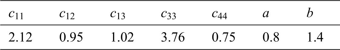
The human bone porosity within the age group 35–40 years is estimated as 0.24 [1]. To evaluate one more poroelastic constant, the following equation is defined MQ=c12c13 in which the value M is not given. Because the fluid is generally isotropic, brr=bzz , the fluid density in the porospace, permeability of the medium, and mass density of the bone take the form of [15] as in Tab. 1.
Table 1: The constants of the material

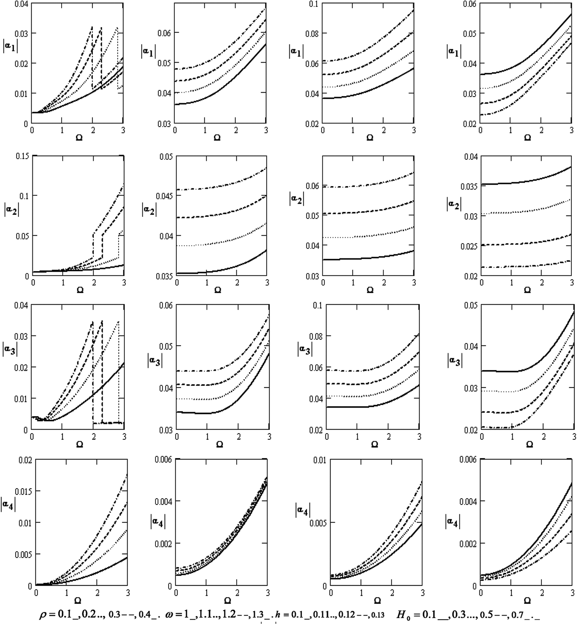
Fig. 1 shows a considerable modification of the absolute value of |α1|,|α2|,|α3| and |α4| coefficients for the poroelastic bones concerning the rotation Ω that increases with increasing rotation for the diverse values of the density ρ , frequency ω, thickness h , and magnetic field H0 . It rises with an increase in the density, frequency, and magnetic field at the effect of density and the coefficients of |α1|,|α3| . It also increases and decreases with the increase of the density.

Figure 1: Variations of the roots |αj|(j=1,2,3,4) concerning the rotation Ω with different values for ρ,ω,handH0
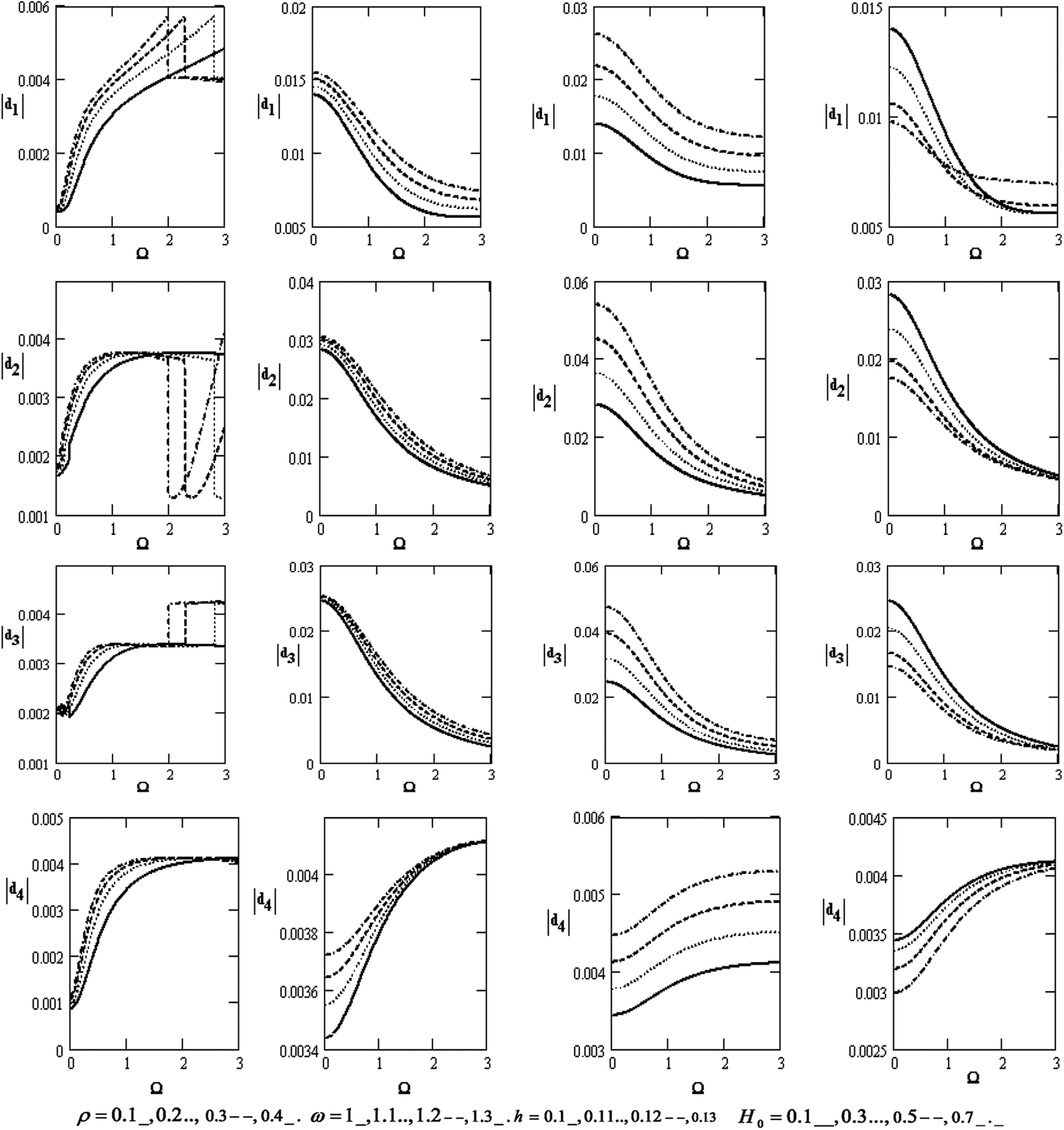
Fig. 2 displays various coefficients of |d1|,|d2|,|d3| and |d4| for the poroelastic bone concerning the rotation Ω , which increases with increasing the rotation for diverse values of the frequency ω, the thickness h , and the magnetic field H0 except for the effect of the density because it increases and decreases. It declines with rising the frequency, thickness, and magnetic field except for the coefficient |d4| that rises with rising the density, frequency, and thickness. Moreover, the coefficients decrease with increasing the magnetic field.
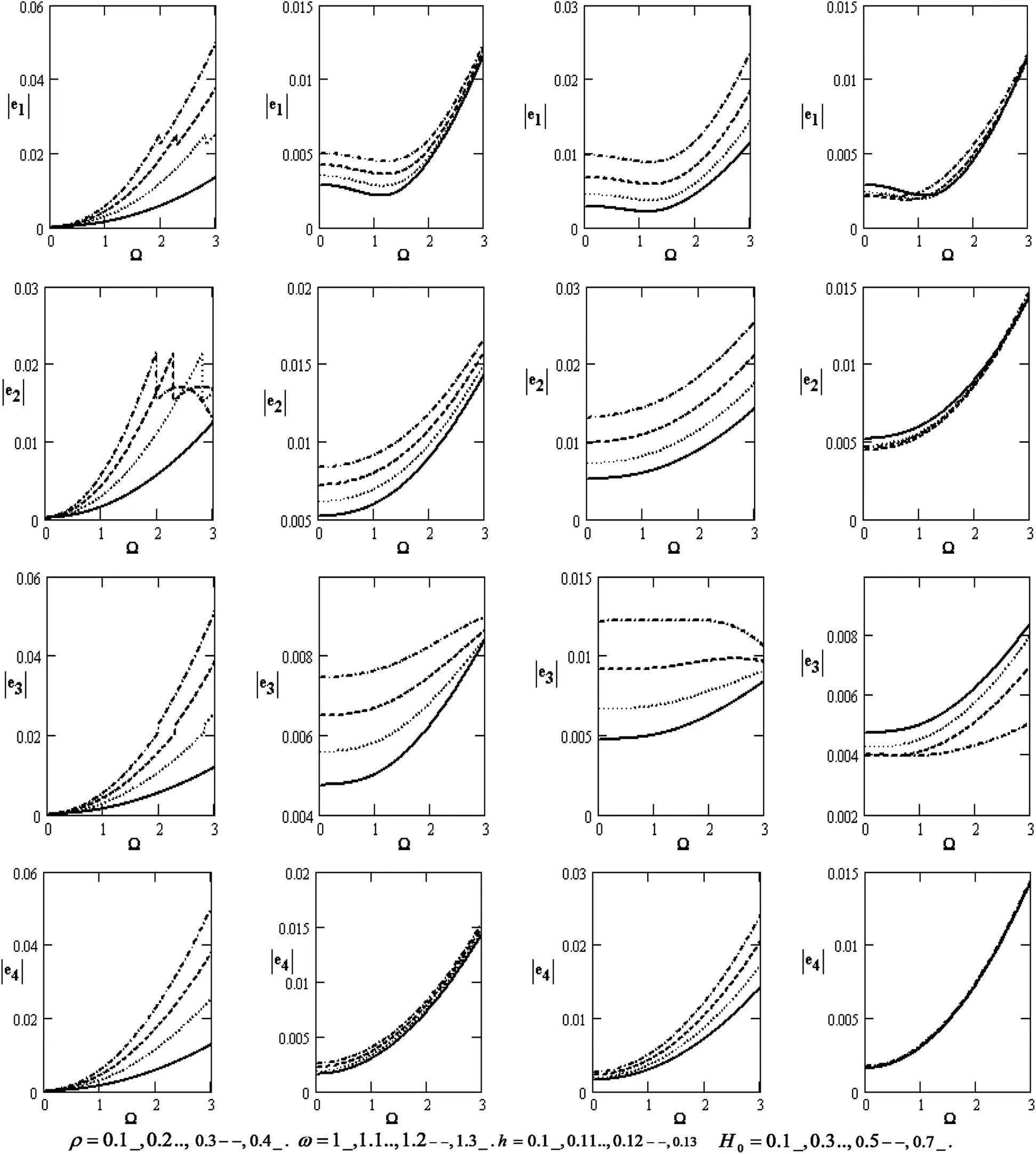
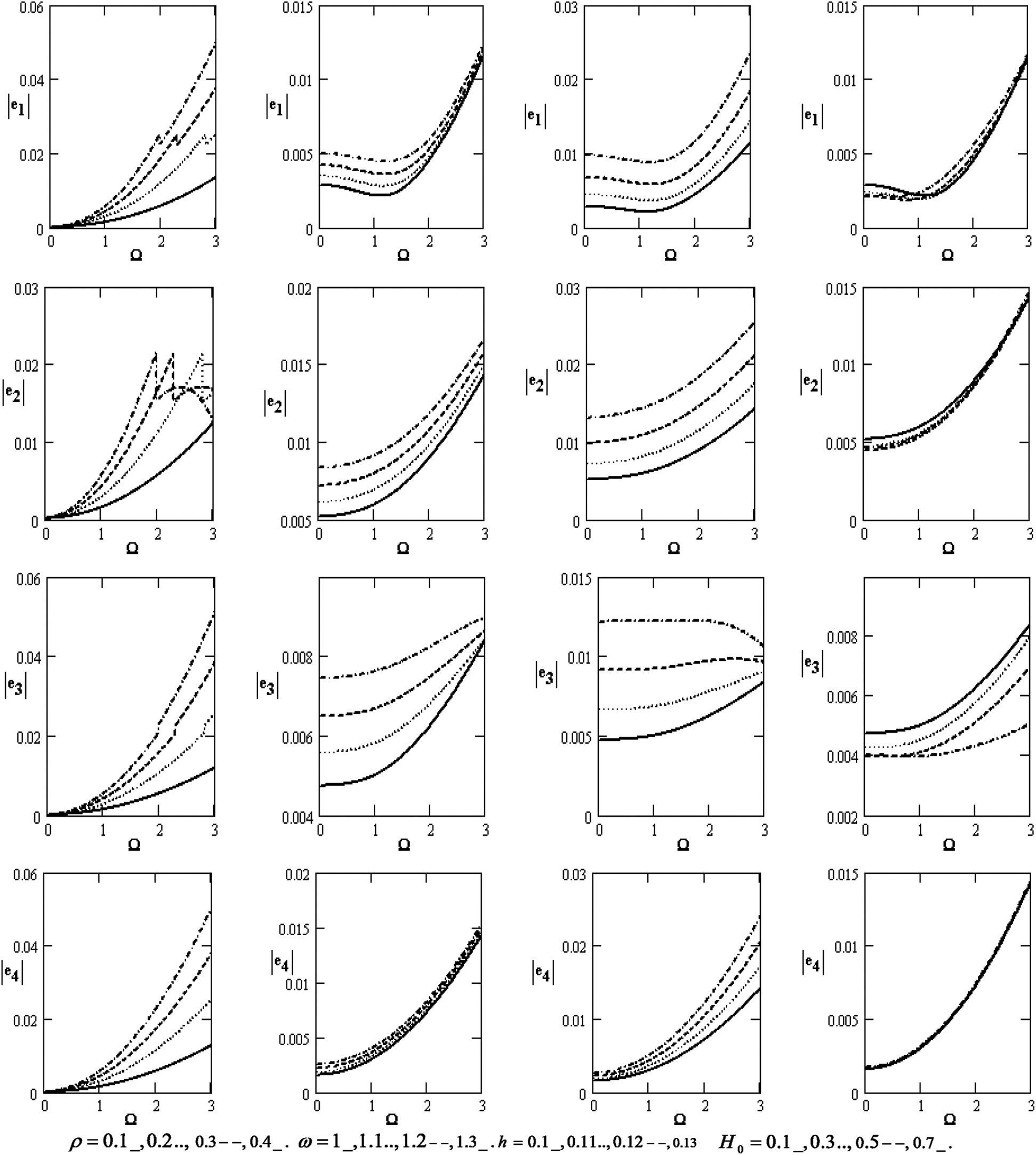
Figure 2: Variations of |ej|(j=1,2,3,4) with respect to the rotation Ω with different values for ρ,ω,handH0
Fig. 3 graphically portrays the variations of the absolute of the coefficients for the poroelastic bone of |e1|,|e2|,|e3| and |e4| concerning the rotation Ω . It rises with rising the rotation for diverse values of the density ρ , the frequency ω, the thickness, and the magnetic field H0 , while it rises with rising the density, frequency, and thickness except for the effect of the magnetic field. In this case, the absolute of the coefficients is the oscillatory behavior in the scope of the Ω -axis for the diverse values of the magnetic field.
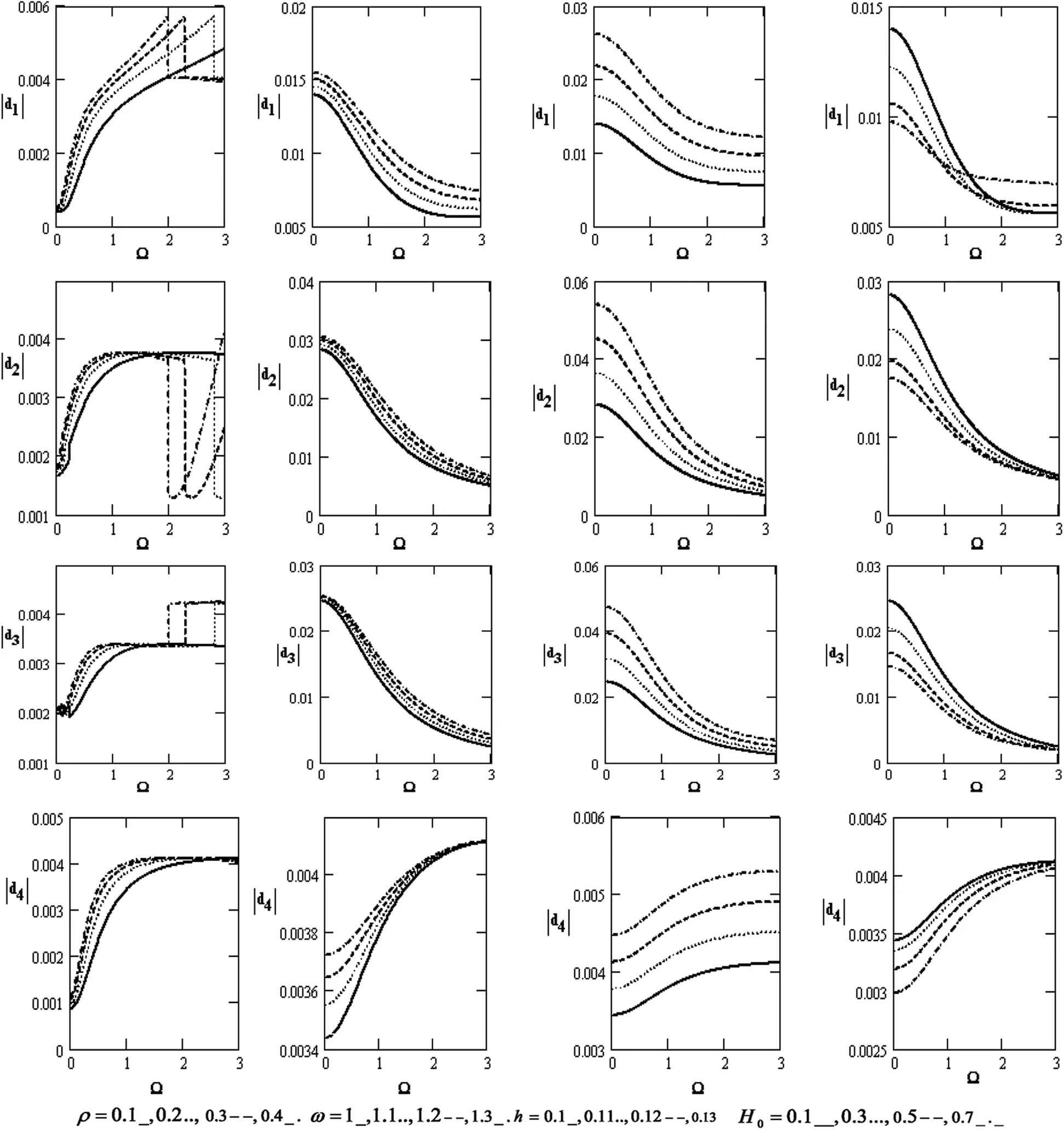
Figure 3: Variations of |dj|(j=1,2,3,4) concerning the rotation Ω with different values for ρ,ω,handH0
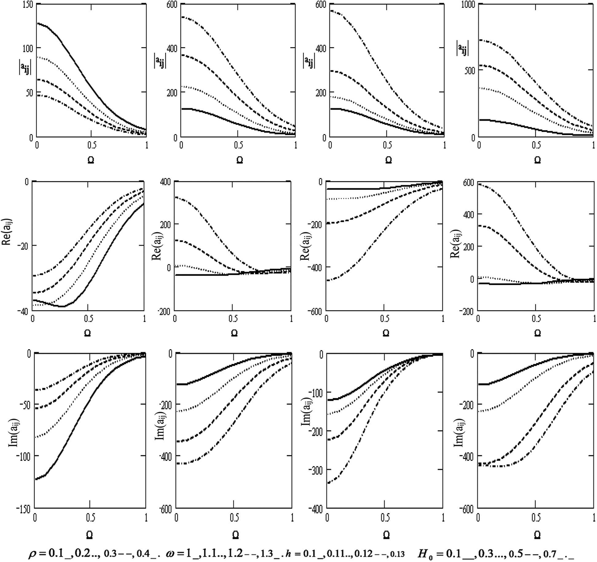
Fig. 4 shows the variations of the scalar equation |aij| , wave velocity Re(|aij|) , and attenuation coefficient Im(|aij|) concerning the rotation Ω for diverse values of the density ρ , the frequency ω, the thickness h , and the magnetic field H0 . It declines with the growing rotation. We also note that the scalar equation increases with the higher frequency, thickness, and magnetic field. On the contrary, it decreases with a higher density. Wave velocity increases with increasing density and rotation. It also rises with the higher frequency and magnetic field but decreases with higher rotation. It declines with higher thickness, and the attenuation coefficient declines with the higher frequency, thickness, magnetic field, and rotation, H0 . Additionally, wave velocity rises with higher rotation and density.

Figure 4: Variations of the determinant |aij|, Re(aij), Im (aij) (i, j = 1,2,3,4) with respect to the rotation Ω with different values for ρ, ω, h and H0
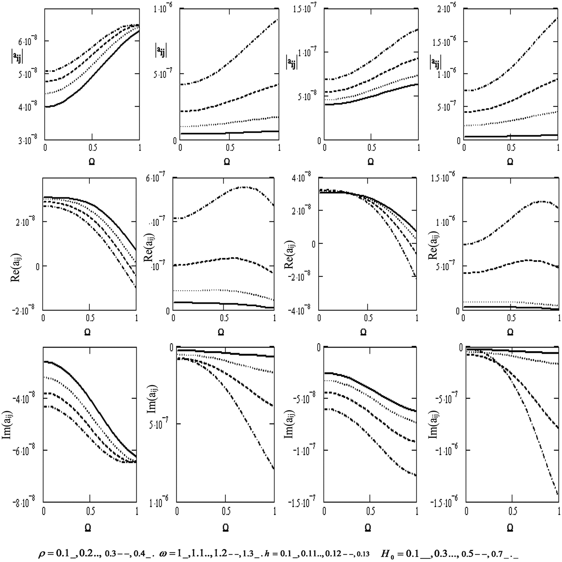
Fig. 5 graphically irradiates the effect of the variations of the scalar equation |aij| , the wave velocity Re(|aij|) , and the attenuation coefficients Im(|aij|) concerning the rotation Ω for diverse values of the density ρ , the frequency ω, the thickness h , and the magnetic field H0 (if the motion is independent of z). The scalar equation rises with higher density, frequency, thickness, magnetic, field, and rotation. Wave velocity rises with higher frequency, thickness, magnetic field, and rotation, except for the effect of the density that rises and declines with higher density. Attenuation coefficients decline with higher density, frequency, thickness, magnetic field, and rotation. They shift downward from positive to negative values.
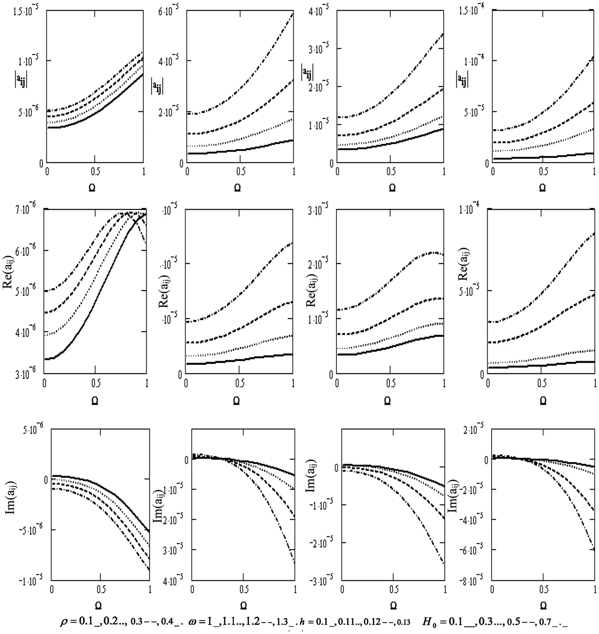
Figure 5: Variations of the determinant |aij|,Re(aij),Im(aij)(i,j=1,2,3,4) with respect to the rotation Ω with different values of ρ,ω,handH0 if the motion is independent of z
Fig. 6 illustrates the variations of the scalar equation |aij| , the wave velocity Re(|aij|) , and the attenuation coefficients Im(|aij|) concerning the rotation Ω for diverse values of the density ρ , the frequency ω, the thickness h , and the magnetic field H0 (if the motion is independent of θ ). The scalar equation rises with higher density, frequency, thickness, magnetic field, and rotation. Wave velocity rises with higher frequency and magnetic field, while it has an oscillatory with the x-axis. However, it declines with higher density, thickness, and rotation. Attenuation coefficients decrease with higher density, frequency, thickness, magnetic field, and rotation. They shift downward from positive to negative values.
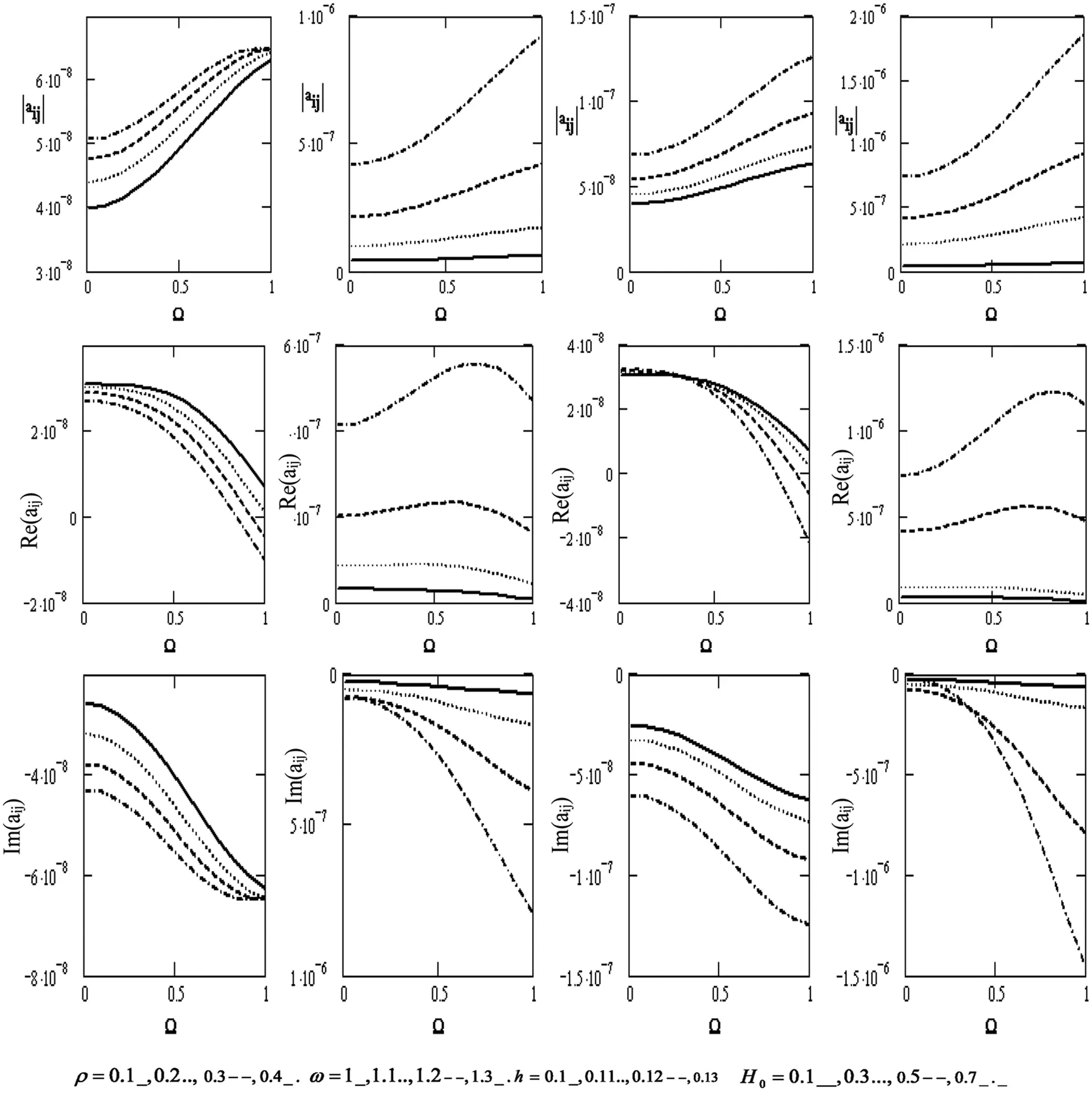
Figure 6: Variations of the determinant |aij|,Re(aij),Im(aij)(i,j=1,2,3,4) with respect to the rotation Ω with different values of ρ,ω,handH0 (if the motion is independent of θ )
Fig. 7 displays the variations of the scalar equation |aij| , the wave velocity Re(|aij|) , and the attenuation coefficients Im(|aij|) concerning the rotation (if the motion is independent of θ and z) for the diverse values of the density ρ , the frequency ω, the thickness h , and the magnetic field H0 . The scalar equation decreases with higher density, frequency, magnetic field, and rotation but declines with higher thickness. Wave velocity rises with higher rotation, density, frequency, and magnetic field, except for the effect of thickness it declines with higher thickness. Moreover, the attenuation coefficient decreases with higher density, frequency, rotation, and magnetic field and rises with higher thickness.
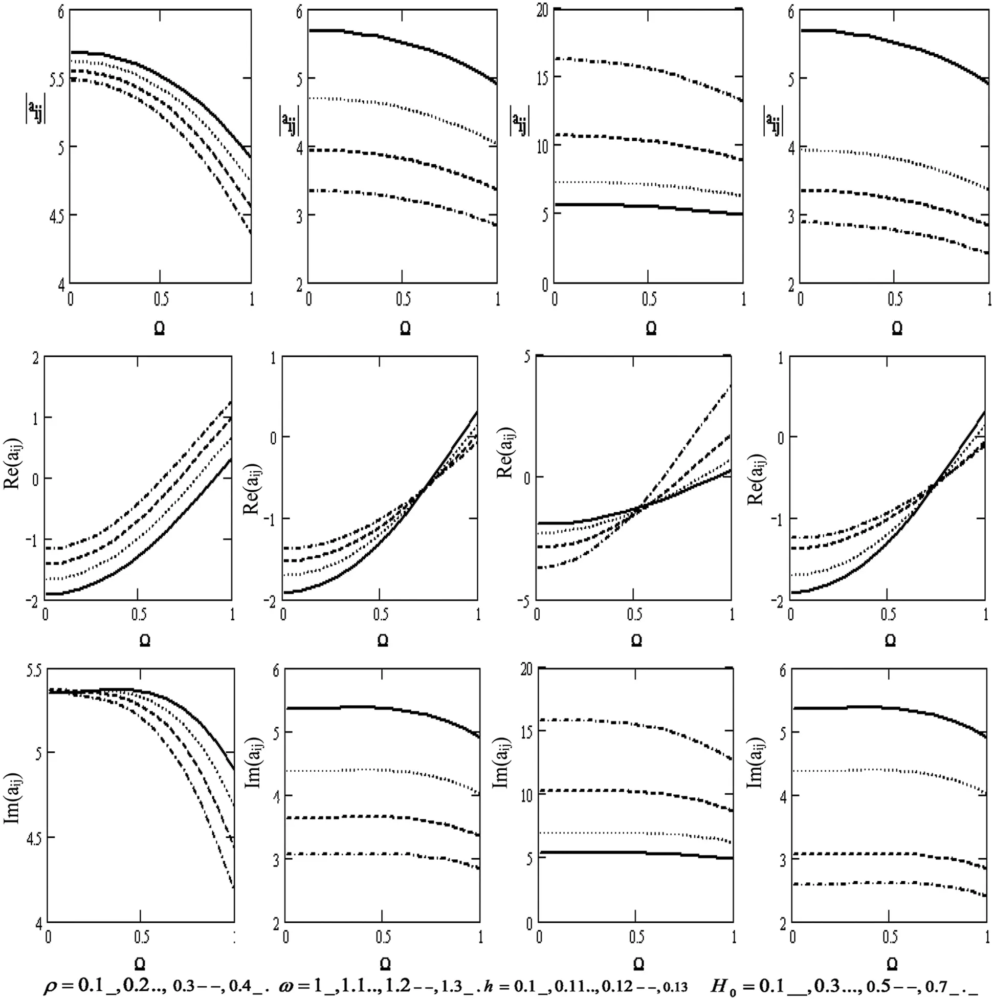
Figure 7: Variations of |aij|=|Δ5||Δ7|,Re(|aij|),Im(|aij|) with respect to the rotation Ω with different values of ρ,ω,handH0 (if the motion independent is of θ and z)