Computers, Materials & Continua DOI:10.32604/cmc.2021.015922
Article

Ozone Depletion Identification in Stratosphere Through Faster Region-Based Convolutional Neural Network

Bakhtawar Aslam1, Ziyad Awadh Alrowaili2, Bushra Khaliq1, Jaweria Manzoor1, Saira Raqeeb1 and Fahad Ahmad3,*

1Department of Computer Sciences, Kinnaird College for Women, Lahore, 54000, Pakistan
2Physics Department, College of Science, Jouf University, Sakaka, Aljouf, 72341, Saudi Arabia
3Department of Basic Sciences, Deanship of Common First Year, Jouf University, Sakaka, Aljouf, 72341, Saudi Arabia
*Corresponding Author: Fahad Ahmad. Email: drfahadahmadmian@gmail.com
Received: 14 December 2020; Accepted: 26 February 2021

Abstract: The concept of classification through deep learning is to build a model that skillfully separates closely-related images dataset into different classes because of diminutive but continuous variations that took place in physical systems over time and effect substantially. This study has made ozone depletion identification through classification using Faster Region-Based Convolutional Neural Network (F-RCNN). The main advantage of F-RCNN is to accumulate the bounding boxes on images to differentiate the depleted and non-depleted regions. Furthermore, image classification’s primary goal is to accurately predict each minutely varied case’s targeted classes in the dataset based on ozone saturation. The permanent changes in climate are of serious concern. The leading causes beyond these destructive variations are ozone layer depletion, greenhouse gas release, deforestation, pollution, water resources contamination, and UV radiation. This research focuses on the prediction by identifying the ozone layer depletion because it causes many health issues, e.g., skin cancer, damage to marine life, crops damage, and impacts on living being’s immune systems. We have tried to classify the ozone images dataset into two major classes, depleted and non-depleted regions, to extract the required persuading features through F-RCNN. Furthermore, CNN has been used for feature extraction in the existing literature, and those extricated diverse RoIs are passed on to the CNN for grouping purposes. It is difficult to manage and differentiate those RoIs after grouping that negatively affects the gathered results. The classification outcomes through F-RCNN approach are proficient and demonstrate that general accuracy lies between 91% to 93% in identifying climate variation through ozone concentration classification, whether the region in the image under consideration is depleted or non-depleted. Our proposed model presented 93% accuracy, and it outperforms the prevailing techniques.

Keywords: Deep learning; image processing; classification; climate variation; ozone layer; depleted region; non-depleted region; UV radiation; faster region-based convolutional neural network

1  Introduction

In 1913, the French physicists Charles Fabry and Henri Buisson discovered the ozone layer. The inorganic compound with the chemical formula O3 is ozone or trioxygen [1]. It is a pale blue gas that strongly smells stingy. It is an oxygen allotrope that, in the lower atmosphere, breaks down to O2 (dioxygen), much less stable than the diatomic allotrope O2. The activity of UV light and electronic discharges into the Earth’s atmosphere shapes ozone from dioxygen. The ozone exists at low concentrations with its peak concentration in the stratosphere’s layer, which absorbs most ultraviolet (UV) radiation in the Sun [2].

In 1930, the British scientist Sydney Chapman identified the photochemical processes that eventually led to the ozone layer. The ozone layer or ozone protection is a stratosphere zone of the earth that blocks the bulk of the ultraviolet radiation of the sun [3]. In contrast to other atmosphere areas, it possesses a high ozone concentration (O3) but weak in following other stratospheric gases. The ozone layer comprises ten parts of ozone per million, while the usual amount of ozone is about 0.3 parts per million in the Earth’s atmosphere as a whole. The ozone layer is located primarily on the lower part of the stratosphere, about 15 to 35 kilometers beyond Earth, although its seasonal and spatial thickness varies [4].

Ozone properties were explored intimately by experimentalist Gordon Miller Bourne Dobson, who established an easy photometer that enabled the relative intensity at two wavelengths to be measured. Dobson also invented a gas O2 that combines to form the O3. The two atoms of oxygen are splits due to the absorption of light and then combine to make the ozone with the third molecule of oxygen. This technique is comprehended as photolysis. These artificial compounds usually occur inside the climate in tiny groups. While associating with an uncontaminated environment, there is a harmony between quantities of gas being made and the ratio of gas being comparable. Thus, the full concentration of gas inside the layer remains relatively consistent [5].

Ozone is a molecule made up of three oxygen atoms (O3) that exists naturally in the stratosphere (topmost atmospheric layer) in small amounts, helping to protect the existence of living beings on earth from the ultraviolet (UV) radiation of the sun. In urban areas, metropolitan cities such as Lahore and Karachi in Pakistan, the thinning of the stratospheric ozone layer is the most significant environmental issue [6]. Chemically, ozone is formed as oxygen molecules absorb ultraviolet photons and undergo chemical reactions known as photodissociation or photolysis. In this process, a single oxygen molecule breaks down into two oxygen (O3) ozone molecules. The ozone layer’s degradation is primarily due to the presence of chlorine and bromine gases such as chlorofluorocarbons (CFCs) and halos, emphasizes [7]. The intensity of ultraviolet light contributes to the dissociation of these gases. Thus, chlorine atoms that precipitate atmospheric ozone molecules are generated. These are also contaminants from cars, by-products of refrigerants for manufacturing processes, and aerosols. Ozone-depleting pollutants are relatively intact in the lower atmosphere leading to the shortening of the Earth’s stratospheric ozone layer. However, they are vulnerable to ultraviolet radiation (UV); consequently, they are dissolved to emit a free chlorine atom. This free chlorine atom interacts with an ozone molecule (O3) and develops a chlorine monoxide (CIO) and an oxygen molecule. CIO is now interfering with an ozone molecule to form a chlorine atom and two oxygen molecules [5]. The free chlorine molecule binds again to the ozone for the formation of chlorine monoxide. The resulting consequence of this continuous phase is the degradation of the ozone layer.

Climate variation is demonstrated as a transformation either within the climate’s mean state or its nonstop variability for an associated period, for decades or longer. The consequences of global climate change are increasing quickly on the economic development of a country like. The Islamic Republic of Pakistan that already have low financial gain and poor human development indicators [8]. Global climate change may occur due to some drastic changes in the Earth’s atmosphere due to destructive activities. The most inducing reason behind global climate change is ozonosphere depletion, the unleash of greenhouse gases, deforestation, pollution, and water resource contamination. It is vital to regulate ozonosphere depletion. Thus, it causes several health problems in humans and animals. Ozone layer depletion surges the volume of UVB that influences the Earth’s surface. Laboratory and epidemiological studies reveal that UVB might cause non-melanoma skin cancer to transform into malignant melanoma [9]. Furthermore, UVB has been connected to cataracts’ growth, a clouding of the eye’s lens, e.g., skin cancer. Ozone depletion also harms biodiversity, ecosystems, marine life, crops and collectively affects the entire system [10,11].

The ozonosphere could be a coating in soil’s stratosphere that comprises comparatively extraordinary absorptions of gas O3. This layer absorbs 93%–99% of the sun’s high-frequency actinic radiation, which is probably damaging to life on Earth. Over ninety-one of the gas in soil’s stratosphere is a gift here. It is mainly situated within the lower portion of the layer from around ten klicks to fifty klicks on top of Earth. However, the thickness differs seasonally and geologically [12]. A French physicist discovered the ozone in 1913. Below, Fig. 1 represents the effect of ozone depletion on the Earth’s atmosphere.

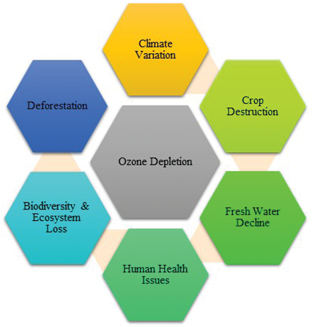
Figure 1: Effects of ozone depletion

Creating a precise prediction model involves collecting input parameters that cause ozone concentration changes [13]. However, due to data source retrieval or significant lost data, much of the desired data is either inaccessible or incomplete [14]. Therefore, a model with a high degree of accuracy needs to be created using a few input parameters.

Various approaches have been implemented to forecast ozone depletion worldwide, such as the deterministic approach and statistical regression. Few approaches have been built based on the principle of linear regression. Multiple linear regression (MLR) is amongst the most prominent linear regression models for estimating ozone depletion. However, the aforementioned models showed a downside in understanding the physical systems’ nonlinearity and complexity [15]. It is desirable to use artificial intelligence techniques, including deep learning techniques that are considerably more powerful and utilize less computing time and resources to detect ozone depletion [16].

To provide a stable prediction process, developments in the neural network model have also been made over the years. By only using meteorological parameters as input data, recurrent architecture increases the efficiency of neural predictors dramatically. Besides, recent research to build a hybrid model focused on a convolutional neural network and long short-term memory (CNN-LSTM) has given an adequate statistical stable hybrid model, and its prediction efficiency has proven to be favorable to a multilayer perceptron (MLP) and long short-term memory (LSTM) [17]. In an attempt to optimize prediction performance and real-time air contamination concentration prediction, the self-adaptive neuro-fuzzy weighted extreme learning machine (SaELM) was explored [18]. On the other hand, Support Vector Machines (SVMs) were unveiled by several experts to estimate ozone saturation in an extended time series fashion [19]. The updated SVM-r model is versatile enough to incorporate other reference variables that may boost forecastings, such as city models or traffic trends. Few kinds of research have centered on forecasting ozone levels in metropolitan environments. The resiliency of Boosted Decision Tree Regression (BDTR) in forecasting ozone concentrations in general and especially in metropolitan centers has not, however, been studied by anyone [20].

In artificial intelligence (AI) terms, Faster Region-based Convolutional Neural Network (F-RCNN) is an advanced form of Convolutional Neural Network (CNN). It is a deep learning algorithm used to detect the images and classify them according to their features [21–23]. It consists of three steps: in the first step, all CNN layers work to extract the appropriate features of an image [24,25]. Then in the second step, the region proposal network (RPN) is a small neural network that acts like a sliding window, performs a feature map function, and predicts either it is an image or not. Finally, in the third step, RCNN is applied to train and test the required dataset, and output is generated accordingly. This technique is employed to improve the actual dataset’s accuracy rate through extensive training and diminishing the loss.

1.1 Problem Statement

The identified issue is a cross-disciplinary topic that falls under a single big umbrella that contains physics, chemistry, mathematics, and computer science. The nonlinearity, complexity, and heterogeneity of the physical systems are sizable barriers in developing trustworthy prediction models for ozone depletion identification based on machine learning or deep learning techniques. It is desirable to use artificial intelligence-based approaches to solve these cross-disciplinary constraints that are considerably powerful with minimal processing time and computing resources to detect ozone depletion areas precisely with improved performance metrics. In fact, in the existing literature, CNN has been used for feature extraction. In that procedure, extricated diverse RoIs passed on to the CNN for the grouping purpose. However, the issue with this procedure is that various images have various prompting areas inside the picture, and it is difficult to manage and differentiate these RoIs that negatively affect the gathered results.

1.2 Objectives

Various approaches have been implemented to forecast ozone depletion worldwide, but this research will contribute by achieving the following objectives:

•    Due to the unavailability of well-organized data source, identification of few reliable input parameters that cause ozone depletion.

•    The creation of a precise prediction model involves identified input parameters.

•    To settle the identified problem by limiting the number of areas in R-CNN.

•    To achieve better results than existing techniques with the help of the proposed approach by fine-tuning of F-RCNN.

This paper is organized as follows. The introduction section presents a brief overview of ozone, the ozone layer, causes of depletion, effects on the ecosystem, developments made in image processing, and deep learning for the precise classification techniques previously used to identify ozone depletion. Section I tackles the problem statement and objectives. The literature review is clarified in section II. Material and methods have been discussed in section III. Validation and results have been represented in section IV. Finally, discussion about the study and results have been discussed in section V.

2  Literature Review

Machine learning and deep learning frameworks have shown massive upgrades in structure and aim to overcome performance-related issues by creating advanced classification models. Physical systems are chaotic in nature, due to which a small change in its input parameters can cause massive transformation in output. Therefore, this section sheds light on the literature regarding different causes of ozone depletion and techniques for the identification of depleted regions in the stratosphere.

In 2019, scientists compared all the regions of China and noticed that North China Plane (NCP) was more affected by air pollution. According to this research, the author observed that there was less research in the past on tropospheric ozone identification and decided to observe nitrogen dioxide NO2, carbon monoxide (CO), sulfur dioxide (SO2), and formaldehyde (HCHO) to determine the density of the troposphere in a vertical column, i.e., dynamical process EI Nino-Southern Oscillation (ENSO), potential vorticity (PV), quasi-biennial oscillation (QBO) and East Asian Summer Monsoon Index (EASMI). The author’s results predicted that troposphere O3 contains changes from increasing to decreasing tendency throughout summer 2005–2016. The author observed all the gas concentrations through satellite and found that these gases’ emission causes a decrease in troposphere O3. The author built a model to analyze the chemical process and dynamic process variables and their effects on troposphere ozone. As a result, the chemical process variable has a 69.73% trend, and the dynamic process variable has a 60.64% observed trend on troposphere ozone in NCP [26].

In 2019, researchers presented a study on troposphere ozone estimation for urban areas [27]. The author observed that ozone depletion in urban areas is increasing due to air pollution [28]. Health agencies can recognize the absorption of the ozone layer. The author used the Artificial Neural Network (ANN) to estimate the ozone layer concentration in Bangi. The input variables are temperature, humidity, UVA, absorption of nitrogen dioxide, and UVB are taken to monitor and record the data [29]. ANN consists of various hidden layers that work behind the scene and measure the ozone layer concentration. This framework gives reliable and adequate assessments of ozone layer absorption [30].

In the same year, estimation was performed in Quito to evaluate the concentration of the ozone layer. The estimation was done by using LUR models with PLS regression. LUR models were used to estimate the concentration of the ozone layer in urban areas [31]. Scientists presented an overview of climate change’s consequences on ozone air quality. Previous analysis has a challenge on how the climate was changed due to variation in the environment. The author observed that the ozone layer depletion increased due to low air quality and caused severe Earth problems. He observed that serious reservations are linked to the meteorological, chemical, and biological processes. In the end, the author concluded that climate variation caused large variations in the environment [32].

In 2018, researchers observed the ozone layer’s surface in China in the past five years (2013–2017) to show severe pollution and its locally flexible tendencies. They resolved the effects of climatological distinctions on ozone through the linear regression model. The primary purpose of that regression model showed increasing ozone tendencies in megacity clusters of China. According to the observations, southern China was considered an area where the ozone depletion rate was high. The estimated rate of NOx emissions in China from 2013–2015 was decreased by 21%. According to the simulations performed through Goddard Earth Observing System Chemical Transport Model (GOES-Chem), the most crucial factor that affected the ozone layer saturation was delicate particle matter (PM2.5). During that particular period, it caused to slow down the level of hydroperoxide (HO2) proportionately [33].

In the same year, the authors developed a model based on ozone concentration using machine learning. Many studies have already been done on climate variation identification, e.g., global warming. Simultaneously, the estimation of overall changes in the ozone layer through fully interactive atmospheric chemistry was expensive. In this research, the authors propose a new technique using a simple linear machine learning-based regression algorithm to calculate the ozone layer absorption. The regression technique helps to calculate the three-dimensional ozone absorption from daily to monthly time intervals. Furthermore, the authors have highlighted the key steps to improve the range of machine learning-based ozone parameters [34].

Researchers in this study presented the chronological subtleties of ground-level ozone and its impacts on Kazakhstan. Due to the increasing air pollution tendencies and their effects on human beings, the authors compared the two cities’ ozone levels. The selected two cities were Almaty and Astana, to figure out the effects of air pollution on the environment. The study was conducted for the concentration of ozone in Almaty on an annual and daily basis and predicted that increasing ozone concentration trends caused severe impacts on the respiratory system in Almaty city. The ozone level became high in a warmer environment, and the emission of gases increased automatically. According to that research, the rate of respiratory diseases in Almaty city was higher than in Astana [35].

Scientists in 2019 worked on increasing trends of stratosphere ozone concentration. It has been observed that the stratosphere ozone is decreasing continuously over the 1998–2016 period. In this research, a space-based analysis of ozone layer concentration was performed. While in space, ozone is decreasing in the hot and even in Northern Hemisphere above 90% approximately. This decrease in ozone layer concentration did not disclose the Montreal Protocol’s ineffectiveness and discussed its positive effects on ozone recovery [36].

A research group in 2019 established a thermodynamic model to measure the concentration of the ozone layer at a low temperature for the first time. The researchers developed a thermodynamic model that measures the ozone layer’s yield when the final gas temperature was equal to the initial temperature and observed that ozone yield increased when the oxygen gas ratio was augmented [37].

Researchers in 2019 predicted ozone layer depletion through remote sensing algorithms. They used two climatologies in this research: Aura Microwave Limb Sounder (MLS) and the other is the Aura Ozone Monitoring Instrument (OMI). These climatologists monitor the ozone concentration every month with longitude (15∘) and latitude (10∘). Their validation is done through a comparison that shows decent arrangements than the previous ozone profile [38].

Four models with six distinct reference variables were explored in this study: Boosted Decision Tree Regression, Neural Network with Gaussian Normalizer, Neural Network with Min-Max Normalizer, and Linear Regression. To choose the correct input parameters for the proposed method, the Pearson Correlation Coefficient was employed. These models were then evaluated in Malaysia at three separate sites. The validity of the proposed model tested by estimating ozone concentrations for various time horizons, 24 hours, and 12 hours, has been examined in two different situations. The outcomes of the models are then compared by adding different performances to test their effectiveness. Finally, concerning the best model, the inconsistencies are calculated using the 95PPU and d-factor bracket indices [20].

A comprehensive discussion of a few prior similar research related to the proposed model’s traits entailed the classification system development based on the ozone concentration.

3  Materials and Methods

Our research supports climate variation management based on identifying the ozone layer’s concentration to predict the depleted and non-depleted regions through Faster Region-based Convolutional Neural Network (F-RCNN). In the existing literature, authors have used Convolution Neural Network (CNN) for feature extraction, where computer vision has become a fascinating field. In that procedure, extricate diverse Regions of Interest (RoI) and pass them to CNN for the grouping purpose. However, the issue with this procedure is that various images have various prompting areas inside the picture that have been extricated in this technique, and it is difficult to manage and differentiate those RoIs that negatively affect the gathered measures.

To solve this issue, a Region-based Convolutional Neural Network (R-CNN) is used that settles the identified issue by limiting the number of areas. R-CNN utilizes a specific search technique to choose a fixed number of RoIs (2000) and considers these regions as the suggested regions. R-CNN’s issue was that it requires some more computing power for preparation and organization due to the bulky grouping of 2000 RoIs for each picture and then learning the patterns. Faster R-CNN is presented to regulate the planning and computational issues; rather than taking care of the considerable number of RoIs to CNN, an information picture is passed to the CNN for the component maps. Highlighted maps help recognize the area of interest; after distinguishing the proposed areas, these areas are wrapped into the square bounding boxes that limit the RoIs. That is why we have used Faster RCNN to predict the depleted and non-depleted regions with bounding boxes.

To completely associate the layer with the corresponding regions, RoI Pooling is utilized to fix their estimate and reshape them for taking care of these regions. At that point, the Softmax layer is utilized in the prospect of class name against each proposed area, and it likewise gives the balance estimations of every region. However, Faster R-CNN’s issue is that when the proposed areas are utilized, they significantly hinder the computing process calculation. The downside of both R-CNN and Faster R-CNN is that they utilize a particular pursuit approach, a tedious method that influences the demonstration of the results [39]. Faster R-CNN has acquainted with to resolve the issues looked in R-CNN [40]. It does not utilize a particular hunt approach; instead, it lets the control learn the identified regions’ features.

Finally, the areas are in order, and every area’s counterbalance estimation is projected [41]. In this research, the Python framework is used for implementation. The primary purpose of choosing Faster RCNN is to differentiate between depleted and non-depleted regions with bounding boxes. The system model flow diagram is shown in Fig. 2.

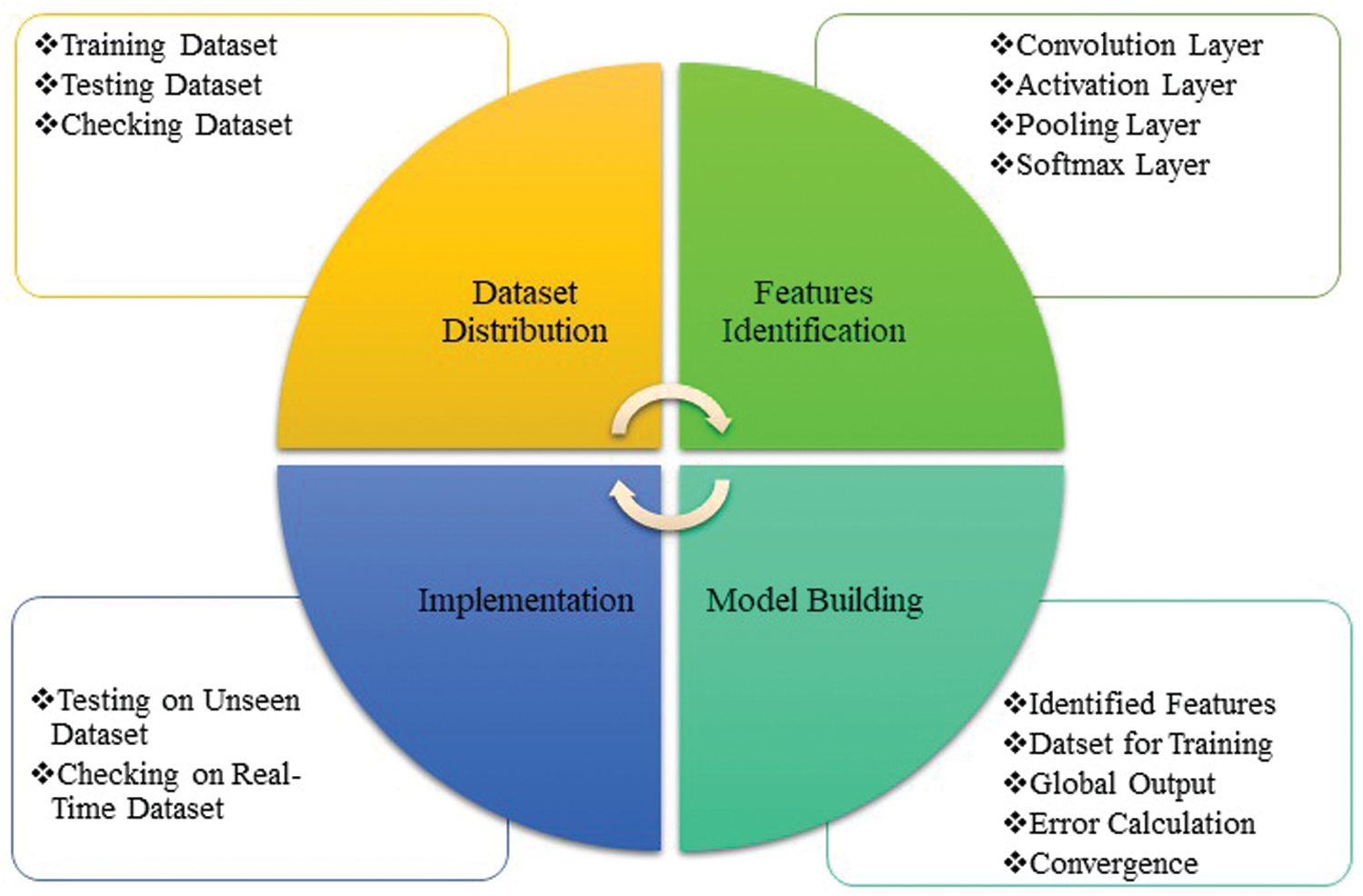
Figure 2: System model

3.1 Backbone Architecture

We have applied F-RCNN in place of a backbone strategy. It consists of various estimated kernel filters. It has eleven channels in the central convolution layer and five channels in the consequent convolution layer, having 3 × 3 different channels. It has 224 × 224 × 3 measurement that is passed to the convolution. At this point, the picture moves through various convolution layers; here, tiny channels of size 3 × 3 are applied to the picture. Occasionally, another 1 × 1 convolution channel is used to protect the measured small pieces collected from original larger pieces. Later, it supports complex learning at the minimum power where different non-linear layers increase the methods’ insight. Five max-pooling layers perform the 3D pooling, and convolution layers always follow these layers. However, all the max-pooling layers are not followed by convolution layers. A kernel of 2 × 2 pixels is used for step two is max pooling. Later on, Convolution layers’ features are transmitted to the RPN, generating proposed regions against detected objects.

RPN gives different proposed regions when it is applied to the images. We can say these proposed regions as CNN feature map sizes. It is an exciting task to work on feature maps having different sizes. To solve this issue, RPN has evolved to map these features and reduce the feature map with the same sizes. However, we know that the max-pooling layer has the same size, but the RoI pooling layer split the feature maps into equivalent regions. After completing RoI pooling, there are three other fully connected layers with 4096 channels in the first two layers. The third layer is responsible for classifying six different techniques for every class of the produced dataset. Thus, we can say that it has six channels for each class. In the end, the SoftMax layer plays an essential role in receiving each class of the dataset. Fully connected always has the same formation in all the systems. Fixed linear components are applied to the hidden layers to add nonlinearity.

In our proposed work, the ozone dataset is taken as input. The dataset is in the form of images; both depleted and non-depleted areas are included. It is essential to normalize the dataset and then place it in a sequence. Furthermore, we have applied Faster RCNN, which consists of three steps, as shown in Fig. 3.

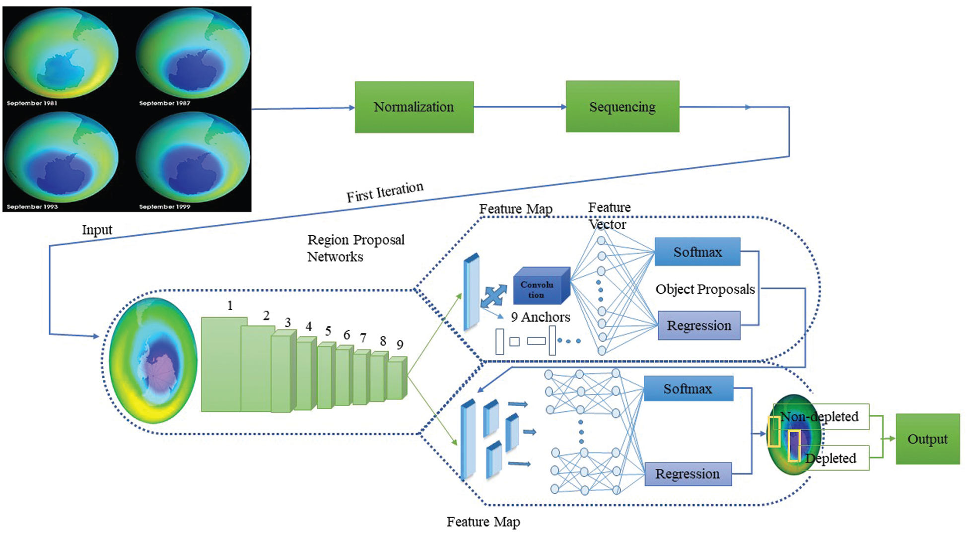
Figure 3: Faster RCNN for ozone layer classification

3.1.1 Faster RCNN

Faster RCNN is presented by Ross Girshick, Shaoqing Ren, Kaiming He, and Jian Sun in 2015. It is a famous object detection architecture and advanced form of CNN. It is a deep learning algorithm used to classify and feature extraction of images after training and testing. It consists of three steps. The network architecture diagram for Faster RCNN is shown in Fig. 4.

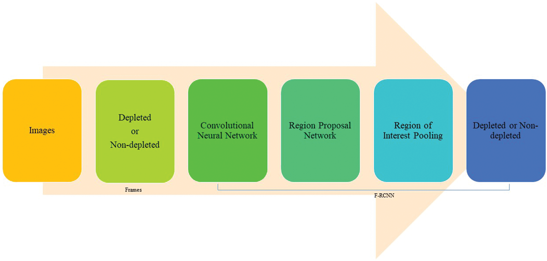
Figure 4: Network architecture of faster RCNN

3.1.2 Convolution Layer

The first step is the processing through convolution layers. Five different layers work behind the scene. According to our scenario, these layers apply convolution, max pooling, and fully connected layers to classify ozone layer images. Filters are trained in this step to extract the appropriate features of ozone images to classify them as depleted and non-depleted areas. The pooling layer is applied to minimize the pixels with low values and consists of a reduced number of features, as shown in Fig. 5. In the end, a fully connected layer classifies those features, which are not under the scope of this research.

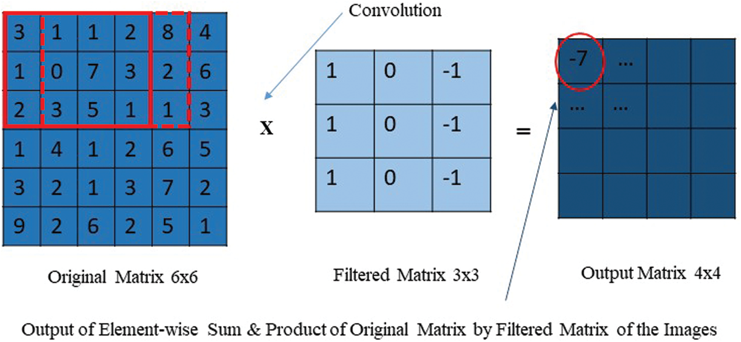
Figure 5: Max pooling

The second step is Region Proposal Network (RPN), in which input images are passed to get the features’ map. The main advantage of RPN is to use weight sharing between the RPN backbone and the Faster RCNN indicator backbone. Bounding boxes are labeled for feature maps. The pooling layer takes that region of the ozone image whose feature mapping needs to be done. RPN is a deep learning algorithm and acts like a sliding window to extract ozone images’ features as depleted and non-depleted regions. When ozone images are passed to the fully connected layer, then their classification and regression branches are served through identified features. These features are then passed through the SoftMax layer to get it done the classification process. Here anchors are represented as boxes, and they can be 3 × 3, 4 × 4, and n × n anchor boxes shown in Fig. 6.

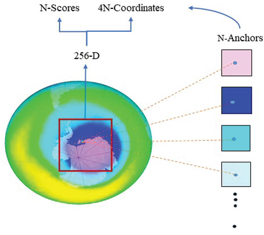
Figure 6: RPN with anchor boxes

3.1.3 Faster RCNN to Predict Image

A fully connected neural network is used to predict the classes and bounding boxes. The ozone images dataset is then learned by the Faster RCNN independently to get the results and accuracy measures. It is used to classify the images into two categories; SoftMax and regression. SoftMax plays a vital role in classifying ozone images and placing the boxes to highlight their depleted and non-depleted regions.

In deep learning algorithms, SoftMax has a great place in the classification of images and appears in logistic regression. We apply SoftMax to obtain output through matrix multiplication. For example, we have a SoftMax, and we denote the vector of logistics as λ. Then we have S(λ): RT→RT. The derivation of this function is presented as follows.

P(W)=S(g(W)) (1)

P(W)=S⋅g(W) (2)

Now applying the multivariate chain rule, the Jacobian of P(W) is

DP(W)=D(S.g(w))=DS(g(W)).Dg(W)S(3)

The Jacobian of g(W) is remaining, here g is a simple function, and calculating its Jacobian is easy. The Jacobian of g(W) has T rows and NT columns.

Dg=[D1G1⋯DNTg1⋮⋱⋮D1GT⋯DNTgT](4)

The weight matrix is linearized to vector length NT. So, we have to linearize in row-major order where all the rows follow each other in ascending order. Precisely Wi, j can get column number (i −1) N+J in Jacobian. To calculate Dg, we recall g1.

g1=W11x1+W12x2+⋯+W1NxN(5)

So,

D1g1=x1D1g2=x2⋯DNg1=xNDN+1g1=0⋯DN+Tg1=0(6)

Now we have the following equation of index W to compute i, j.

Dijgt=Wt1x1+Wt2x2+⋯+WTNxN/Wij={(xji=t0i≠t)(7)

The dot product between row DS and column Dj is the following.

DijPt=DiStxj(8)

The above equation shows that we can compute the SoftMax without actual Jacobian matrix multiplication and alternatively we can calculate the SoftMax through the following formula. The complete description of this formula is given in Fig. 7.

P(yi∣xi;W)=efyi∑ jefj(9)

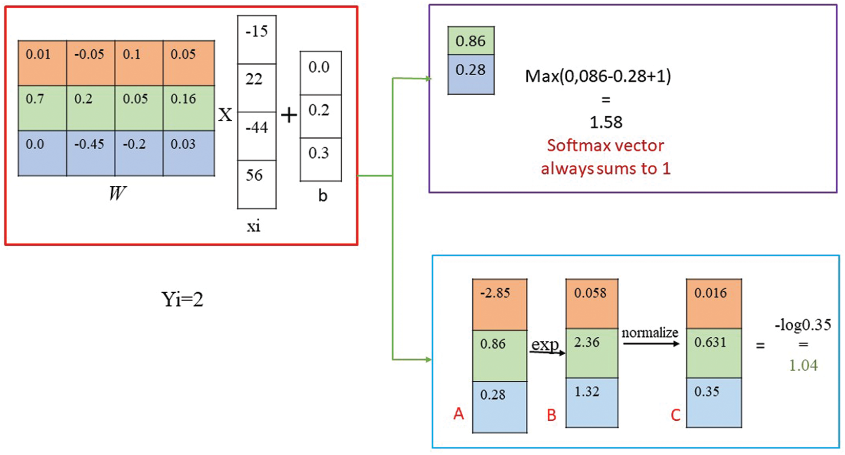
Figure 7: Mathematical derivation of SoftMax

4  Simulation and Result Discussion

Faster RCNN follows a supervised learning approach, and due to some certain constraints and limitations we collected 200 images for the ozone depletion identification. Then, a python script has been developed for the augmentation of dataset, which is the primary requirement of the proposed model for the better capacity building. Augmentation process increases the number of images from 200 to 500. Overall, implementation is done in python using YOLOv3 for Faster RCNN. The accuracy rate is increased after every iteration. For labeling all datasets, we used label-mg, which is a desktop application. We applied label-mg to distinguish between depleted and non-depleted regions. When we applied label-mg on images, it converts the JPEG and PNG images into the XML file. In the XML file, we have all the images, which are labeled by us plus our values against it. After labeling all the images, Faster RCNN implementation is done that it is used for the classification and detection of images at a high accuracy.

A dataset of ozone layer comprising depleted and non-depleted regions is generated on our own to feed the proposed algorithm. The dataset contains almost 2000 images generated by us by applying annotation on images to label images. Five hundred images are collected for each class, and we have a total of two classes as shown in Tab. 1; the width and height of every triangle are scaled again to 256. One of the significant goals in training the deep learning network is that average loss should be minimized by looking out the best parameters. The learning rate for the first 10,000 epochs is set to 101, and it gets incremented after every 20,000 epochs in the deployed system. Stochastic Gradient Descent (SGD) is used for weight optimization during backpropagation. To prevent overfitting, early stop function is deployed as overfitting is one of the significant factors that distress the system performance. When the model tries to learn noise and other hidden details in training data, overfitting happens and negatively affects system performance.

Table 1: Dataset distribution

First of all, we have uploaded 500 images for training purposes and obtained a 90% accuracy rate. To increase proposed model’s accuracy rate, dataset is tested in the second iteration and got accuracy 92% and 90% for depleted and non-depleted regions respectively. The popular loss function (Mean Square Error) is used for the calculation of system’s overall loss. In Fig. 12, we have shown the training and validation loss.

The overall calculation of loss is shown in Eq. (10); it is calculated after calculating the difference between every data point and dividing this by total data points.

MSE=∑t=1vJt=J(Sj-Sjp)2V(10)

Here t is the number of data points available from 1 to v, Sj is the actual label, Sjp is the predicted label. The total accuracy is 93% in our proposed system. Training and validation accuracy is displayed in Fig. 11.

Yu Chen Wang used the SVM classifier with the self-generated dataset and achieved 91% accuracy. Also, Xinchen Wang used the Faster RCNN with a Pascal VOC dataset and achieved 90.6% accuracy. We evaluated and compared our results with different existing architectures. The comparison of our results with the architectures mentioned above is displayed in Tab. 2.

Table 2: Comparative analysis

Faster R-CNN based detection and classification. Fig. 8 indicates the 90% accuracy for the depleted region during training phase. Furthermore, the accuracy during training is 92% for the non-depleted regions, as shown in Fig. 9 below.

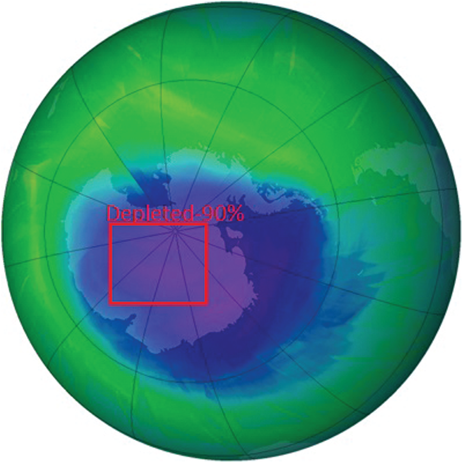
Figure 8: Accuracy of depleted image during training phase

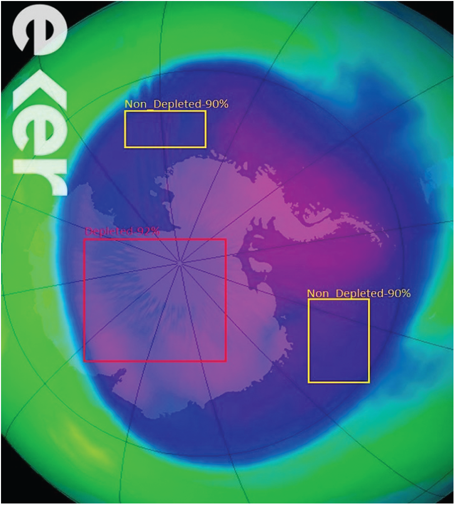
Figure 9: Improved accuracy for depleted and non-depleted regions

Our identified system Faster RCNN achieved a overall accuracy of 93% during testing by using self-generated dataset. Fig. 10 shows the improved accuracy rate for the depleted region from 90% to 93%, while for the non-depleted region from 90% to 91%.

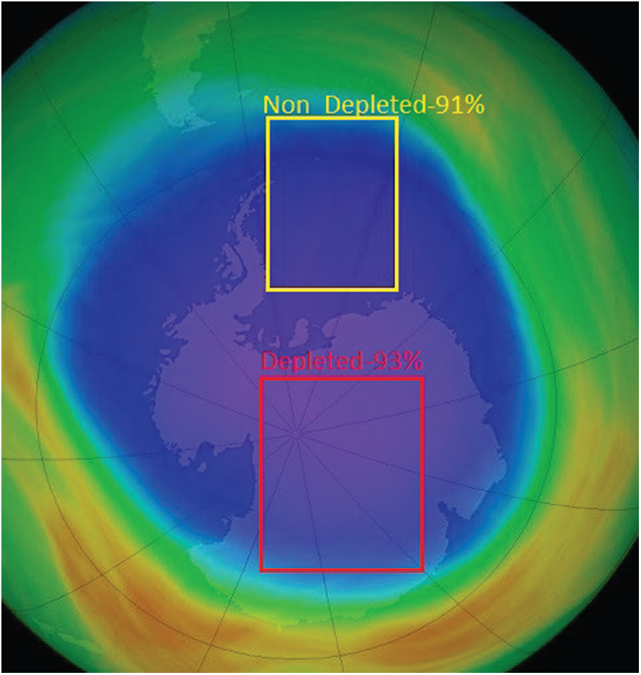
Figure 10: Improved accuracy of testing during validation

Finally, in the third iteration, the accuracy rate for both depleted and non-depleted regions has been increased. In this iteration, the depleted region’s accuracy is 93% and 91% for the non-depleted region.

The number of epochs for training and the validation are 200,000, at which reliable and significant results were obtained. Fig. 11 shows the difference between the training and validation accuracy of our proposed model. We can observe that overall validation and training accuracy is more than 90%. Similarly, Fig. 12 shows the difference between the training and validation loss that is getting smaller as the number of iterations increases. Therefore, we can say that identified technique has performed well.

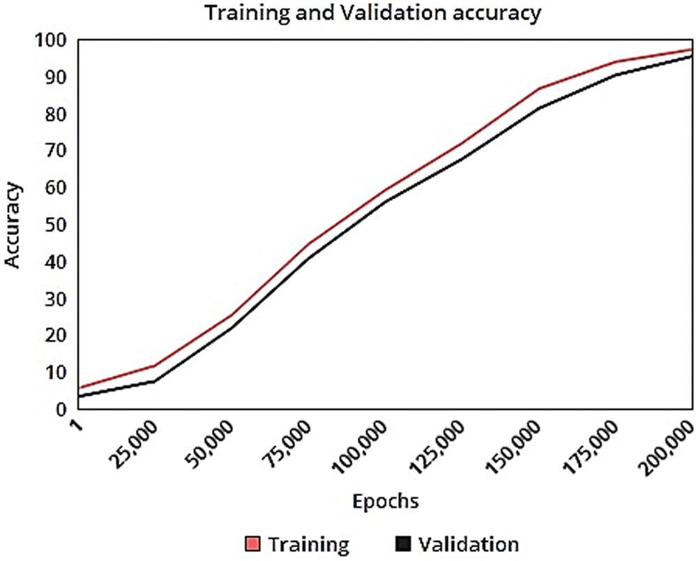
Figure 11: Training and validation accuracy

5  Discussion

The classification goal in deep learning is to predict the identified classes accurately for every presented case in the specified domain [42]. The most well-known deep learning technique is CNN, which predicts the images’ classes based on extensive training. Here we have taken the ozone images-based dataset. This paper has used F-RCNN, an advanced technique based on CNN using the ozone layer images dataset to predict the depleted and non-depleted regions. Our proposed system proved to achieve an overall accuracy of 93% during the training and testing phases through experimentation and validation. Researchers used the SVM classifier, and the results generated shown that they attained 91% accuracy [20]. Another research group used the F-RCNN technique over the Pascal VOC dataset, and they achieved 90.6% accuracy in detection and classification [43,44]. In this study, the identified F-RCNN technique has used our self-contained dataset consisting of ozone images with (250 × 250) size each. Finally, we got 93% accuracy, which is better than the techniques used in previous studies. The main advantage of F-RCNN is to accumulate the bounding boxes on images to differentiate the depleted and non-depleted regions. It depicts our fine-tuned model out-performs than other architectures in terms of accuracy and loss measures.

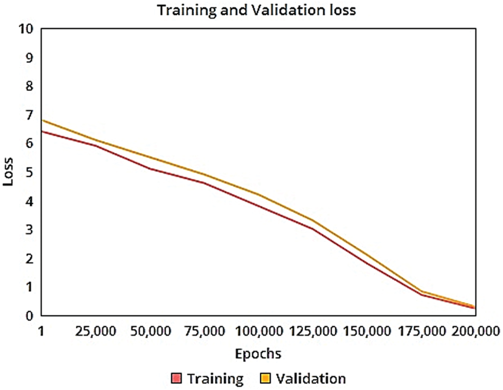
Figure 12: Training and validation loss

In conclusion, the anticipated deep learning-based classification model F-RCNN is deployed to monitor ozone in the stratosphere by detecting depleted and non-depleted regions for future environment-related policies and the betterment of ecology. Dataset has been created that incorporates current stratosphere images of two types based on ozone depletion and non-depletion. The dataset contains 28 features and two classes. The python platform is utilized in this work as it can work with high certainty because of its capability of creating authentic outcomes that mirror a specific domain of intelligence. The deep learning algorithm-RCNN was applied to the self-generated dataset for classification in two groups precisely: that have different ozone concentration levels. It will help to characterize the normal ozone concentration to ensure proper monitoring of climate variation and slow down the adversative changes by making prolific policies to maintain appropriate ozone levels.

Due to the research scope, some common types of image datasets and parameters have been selected, but in the future more categories of innovative images and features in the stratosphere can be incorporated to better understand and cope with the issues. Furthermore, innovative algorithms can also be designed, or existing ones can be modified to detect a broader range of variations in the dataset in order to get better efficiency and accuracy.

Acknowledgement: Thanks to our colleagues & institutes, who supported us morally.

Funding Statement: The authors received no specific funding for this study.

Conflicts of Interest: The authors declare that they have no conflicts of interest to report regarding the present study.

This work is licensed under a Creative Commons Attribution 4.0 International License, which permits unrestricted use, distribution, and reproduction in any medium, provided the original work is properly cited.