DOI:10.32604/cmc.2021.016678
| Computers, Materials & Continua DOI:10.32604/cmc.2021.016678 | |
| Article |
An Adaptive Anomaly Detection Algorithm Based on CFSFDP
1School of Computer Science and Technology, Changchun University of Science and Technology, Changchun, 130022, China
2SRoom 657, J.T.Patterson Labs Bldg.(PAT), Austin, 78712, TX, USA
*Corresponding Author: Weiwu Ren. Email: renww339@163.com
Received: 08 January 2021; Accepted: 15 February 2021
Abstract: CFSFDP (Clustering by fast search and find of density peak) is a simple and crisp density clustering algorithm. It does not only have the advantages of density clustering algorithm, but also can find the peak of cluster automatically. However, the lack of adaptability makes it difficult to apply in intrusion detection. The new input cannot be updated in time to the existing profiles, and rebuilding profiles would waste a lot of time and computation. Therefore, an adaptive anomaly detection algorithm based on CFSFDP is proposed in this paper. By analyzing the influence of new input on center, edge and discrete points, the adaptive problem mainly focuses on processing with the generation of new cluster by new input. The improved algorithm can integrate new input into the existing clustering without changing the original profiles. Meanwhile, the improved algorithm takes the advantage of multi-core parallel computing to deal with redundant computing. A large number of experiments on intrusion detection on Android platform and KDDCUP 1999 show that the improved algorithm can update the profiles adaptively without affecting the original detection performance. Compared with the other classical algorithms, the improved algorithm based on CFSFDP has the good basic performance and more room of improvement.
Keywords: Anomaly detection; density clustering; original profiles; adaptive profiles
Intrusion detection is an effective defense technology in network security. Since it was proposed in 1980, intrusion detection has been highly concerned by the industry and academia. In recent years, with the development of artificial intelligence, intrusion detection has also developed in the area of intelligence. Some new algorithms have been applied to the field of intrusion detection. Shone et al. [1] proposed a deep learning technique for intrusion detection, which addresses the feasibility and sustainability of current model for modern networks. Chawala et al. [2] proposed intrusion detection with combined CNN/RNN model, which described anomaly by RNN and improved anomaly IDS by CNN with GRUs. Alrawashdeh et al. [3] proposed an anomaly detection based on RBM and implemented a deep belief network.
According to different principles, intrusion detection system can be divided into two categories: intrusion detection based on misuse and intrusion detection based on anomaly. Misuse detection can effectively detect known attacks, but not unknown attacks. Anomaly detection can detect unknown attacks, but it is often plagued by false alarm rate. In addition, intrusion detection usually needs to label the data before training. Labeling does not only need a great deal of expert knowledge, but also costs a large number of resources. At present, there is not enough fresh data set for training in the field of intrusion detection system.
In order to reduce the false alarm rate of anomaly detection, it is necessary to design and implement the algorithms that have good profiles naturally, such as SVM, Adaboost and random forest. In order to reduce the dependence on labeling data, there are two main methods: one is to use easily extracted data such as normal behaviors as training data; the other is to use unsupervised or weak supervised algorithm for training.
Clustering algorithm, as a natural high-precision, unsupervised machine learning method, has been widely introduced and applied to the field of the anomaly detection. Density clustering can find cluster of arbitrary shape, not just “quasi-circular” clustering. Therefore, density clustering has natural advantages in accurately describing profiles. Some improved algorithms [4] have the ability to resist noise. Shamshirband et al. [5] used a density-based clustering algorithm to form arbitrary cluster shapes for improving their proposed algorithm. However, compared with other clustering methods, density clustering has high storage and computational costs. The main reason is the lack of effective data structure to store and retrieve clustering information. Kalle et al. [6] proposed an anomaly detection algorithm based on hierarchical clustering. Two mechanisms for adaptive evolution are introduced: incremental extension with new elements of normal behavior, and a new feature that enables forgetting of outdated elements of normal behavior. In addition to incremental capacity, this algorithm not only guarantees detection performance, but also has good real-time performance. The principle of partitioning clustering is simple and easy to understand. But the detection performances of its improved algorithms are so different. Gargand et al. [7] used a combination of fuzzy K-means clustering algorithm, extended Kalman filter, and support vector machines to detect the anomalies. The best set of features is computed by fuzzy k-means algorithm. Gu et al. [8] proposed a semi-supervised clustering detection method using multiple features. The proposed Multiple-Features-Based Constrained-K-Means (MF-CKM) algorithm can solve three problems: large numbers of labeled data, the relatively low detection accuracy and convergence speed of unsupervised K-means algorithm. Additionally, Velea et al. [9] detected anomalous behavior in network traffic through parallel K-means clustering. This method does not need to inspect users’ data package and can protect users’ privacy. Zou et al. [10] used the K-means clustering algorithm of data mining for logs to construct the normal behavior library so as to distinguish between normal behavior and abnormal behavior. In general, the study of anomaly detection based on partition clustering gives rise to two main difficulties: one is the selection of parameter k, the other is enlarging the partition between normal and anomaly. In their methods, the above two problems must be handled at the same time so that the algorithm based on partition clustering can achieve good detection performance. The grid clustering divides the data space into a grid structure of finite cells, and organizes a series of adjacent high-density cells into profiles. This method does not store each feature points but store the cell, that is, the statistics of feature data. Later on, Dromard et al. [11] proposed an incremental grid clustering to detect rapidly the anomalies. But how to select the right cell granularity is a problem. At the same time, some other clustering methods are also applied to intrusion detection, such as graph clustering method [12].
To sum up, clustering is a very good non-supervised anomaly detection method. Every method has its advantages and disadvantages. Density clustering can find any shape of cluster, which has a natural advantage in the description of the profile. Therefore, density clustering has always been a hotspot in the application research of clustering in anomaly detection. However, anomaly detection based on density clustering has three kinds of problems [13]: the first is the difficulty of determining the neighborhood range due to the uniform density; the second is parameter modifications that would cause instability of the model; while the third is real-time problem caused by too much computing overhead. In addition, clustering, especially density clustering, is difficult to adapt profiles with new input. Such a tiny part of studies show positive results about the adaptive profiles, whereas most studies do not involve or have negative results.
CFSFDP [14], i.e., Clustering by fast search and find of density peak is a simple and crisp density clustering algorithm. It can find possible clustering center itself by defining local density and distance. It can solve the difficult problem of determining the neighborhood range through one parameter. It is a very robust algorithm. However, CFSFDP is not designed for anomaly detection. CFSFDP can build a clustering, but if it is the new input after clustering, it is unable to be added to the existing clustering, and is not capable of changing the existing clustering. For intrusion detection, especially the model with network behavior as input, it needs to constantly modify its own model to adapt to the new attack detection, but there is no such theory or application at present.
In this paper, an anomaly detection algorithm based on CFSFDP is proposed. It can solve the dynamic adaptation of anomaly detection model based on CFSFDP. New input may affect the shape of clustering, and then change the existing model. We consider the possible results of all the inputs, and build new behavior profiles based on these results. Under the setting that the existing model is not changed as far as possible, the generated new cluster is fused with the existing model to obtain the adaptive detection performance. Meanwhile, the complex computation of clustering information can also be optimized by parallel computation.
Definition 1. Support radius dc: dc > 0, is the support radius, if
Definition 2. Center point Ccl: the original center point of cluster, where C is the identification of center point and cl is the cluster identification. cls represents all clusters.
Definition 3. Edge point Ecl: the points belong to cluster but not in the radius of dc are edge of clusters, and they can be defined as Ecl, where E is the edge identification.
Definition 4. Discrete point D : the points that do not belong to any cluster are the discrete points, which can be defined as D.
Definition 5. Distance
Definition 6. Distance
Definition 7. Distance
Definition 8. The robbing function
Definition 9. The selecting factor
where
Definition 10. Center step degree STC: the equation of STC is
where
Definition 11. Discrete step degree STD: the equation of STD is
where
The main idea is to analyze the relationship between the new input and the existing clustering, that is, the possible results of adding new input to the existing clustering. There are three possible results: the first is that the new input may expand the boundary of the existing clustering; the second is that the new input may change the subordination of the edge points; the third is that the new input may generate new clusters. It will be very challenging to solve the model adaptability from these three possible results.
Our basic idea is to decompose the complex adaptive problem into several three problems: one is the relationship between a new input and one known cluster; the second, the relationship between a new input and two known clusters; and the third, the relationship between a new input and multiple known clusters. As shown in Fig. 1, it is the relationship between a new input and one known cluster. The red point represents the new input, the solid circle represents the radius dc of the known cluster, and the points within the solid circle belong to clustering, while in Fig. 1a, the dark yellow point is within the cluster. The purple dashed circle represents the range controlled by the cluster, the edge point is between the solid circle and the dashed circle, and cl1 represents the number of cluster. There are three possible scenarios for this problem: the first scenario is that the new input is within the radius of the known cluster, as Fig. 1a depicts, the new input is within the radius of the cluster, which will directly affect the cluster. According to our definition of edge points, the density of the cluster center will lead to the increase of the density. The density increase of cluster leads to the expansion of cluster range, and some new edge points are added, which are the light yellow points in Fig. 1a; the second scenario is that the new input is outside the radius of cluster, and will be the edge point of some cluster. Just as Fig. 1b illustrates, according to the calculation, the new input, namely the red point, will become the edge point of cluster. It will not directly affect the clustering; the third scenario is that the new input is outside the radius of class, and will be the discrete point of the class. It will also not directly affect clustering.

Figure 1: The relationship between a new input and one center (a) A new input in the cluster cl1 (b) A new input on the edge of the cluster cl1 (c) A new input separated from the cluster cl1
There are two representative scenarios of the relationship between a new input and two known clusters. One scenario is that the new input is the edge point of the current cluster. As shown in Fig. 2a, the new input, namely the red point, falls into the edge range of cluster cl1. It can be visualized in Fig. 2, but in fact, we are directly incapable to judge which cluster the point belongs to. And it needs to be judged by calculating which cluster has more influence; the other is that the new input is within the radius of two clusters, as is shown in Fig. 2b, the new input will increase the density of the current cluster, and more edge points will be included.

Figure 2: The relationship between a new input and two centers (a) A new input on the edge of the cluster cl1 (b) A new input in the cluster cl1
What Fig. 3 displays is the relation between a new input and several known clusters. Since we have already discussed the situation about the new input becoming edge or discrete point, here we mainly discuss the new input and its surrounding points may be clustered as a new cluster, which is also the most complex situation. In Fig. 3, with the black pot representing the discrete point, the blue pot representing the edge of cluster cl2, and the yellow pot representing the edge of cluster cl1. The new input, namely red pot, falls into the middle of the edge points and the discrete points. The density in the radius of new input is enough, in addition, the distances between the new input and the other center of clusters are enough, so it will generate a new cluster. It should not be intuitive and be judged by calculating density and distance.

Figure 3: The relationship between a new input and multiple-centers
According to the analysis of Section 3, we can conclude that the key is to find the relationship between the new input and the original cluster, especially the relationship between the new input and the original cluster when it may be the new cluster. As shown in the Fig. 4, the process of algorithm can be divided into three parts: the first, to calculate the distance and density and store all kinds of information between the new input and the original cluster; the second, to judge whether the new input to be the new cluster or not; the third, to assign the new input to its nature identity, whether it is the center, edge or discrete point. And the points which are affected by new input should be reassigned. The following logic is needed to judge whether the new input to be a new cluster or not: firstly, the new center must not be within the radius of the original cluster; secondly, the density of the new input in the radius should be enough; thirdly, the distance between the new input band the other original cluster center should be enough. Based on these logics, the following judgment is needed: the first is to judge whether the new input to be within the radius of the original cluster or not. If in the radius, the new input cannot be the center; the second is to calculate the density and the distance. The density is the number of points in the radius of new input. If the density is enough, then it should be calculated the distances between the new input and the center of the other clusters; the third is to judge the new input to be a new cluster or not. We defined a cluster center selection factor that includes two indicators: density and distance. Once the current i of the new input is large than the original lowest
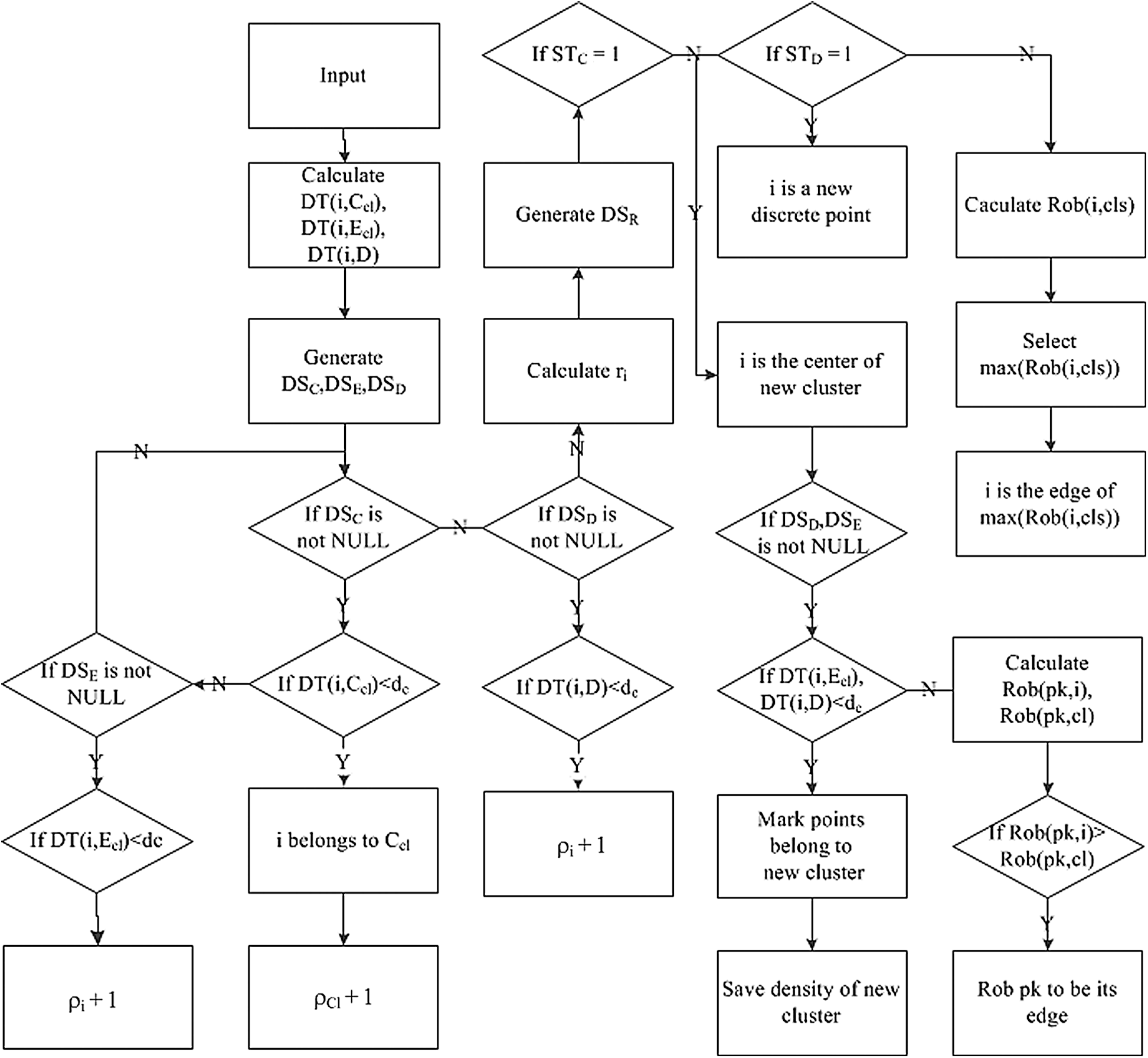
Figure 4: The flow chart of adaptive CFSFDP algorithm
In addition, for the new input which does not belong to the cluster and will also not be a new cluster, it is necessary to give priority to judge whether it be a discrete point or not. Because the discrete points are usually noise, they have great influence on the performance of detection. In this paper, we define the discrete points strictly. We consider that the discrete points are the same as the center points, and there are significant differences with other points. So the purpose of our definition is to distinguish the noise and the profile better. The new input is neither a cluster center nor a discrete point, hence it can be assigned to the edge point. The rob factor should be calculated, and the new input belongs to the cluster which has the largest the rob factor, that is, the cluster robs this new input.
The following logic is needed to judge which nature identity the new input should be assigned to: the first logic is that when the new input generates a cluster, it will rob edge points from other clusters; the second, when the new input is a discrete point, it will have no influence on profiles and be marked as a discrete point; the third, when the new input is within the radius of center, it will increase the density of the current cluster and be marked as cluster identification. Although increasing the density continuously may lead to the change of center or even the profile, in fact, the profile has not changed too much. For simplicity and stability, our strategy of designing algorithm is to keep the original profiles as much as possible. Therefore, increasing the density in the original cluster is ignored; the fourth, when new input is an edge point, it will calculate the distances to other center points, then calculate the rob factors, and judge which cluster it belongs to.
Here we do not discuss the algorithms of building normal profiles and anomaly detection, mainly because this part is proposed in another paper [15]. The basis of anomaly detection is that the normal behaviors have certain regularity and similarity. In that paper, it is concluded that the clustering profiles are composed of the center points and their support radiuses. Within the profiles, it is considered as the normal, otherwise is anomaly.
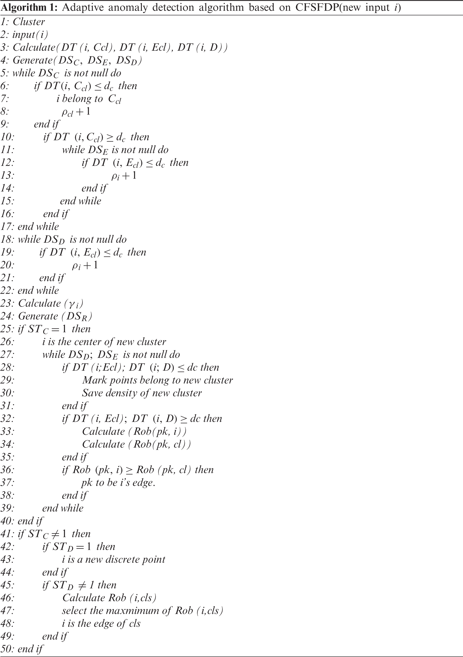
The pseudocode of generating profiles is as follows:
The experimental data includes two parts: one is from the open data set KDDCUP 1999 of intrusion detection; the other is from the data extracted by the mobile anomaly detection system based on Android that we developed. We will do two groups of experiments: one is the comparison between our improved algorithm and the other algorithms on the open data set, and the other is the comparison between our improved algorithm and other algorithms on data set that extracted by mobile anomaly detection system. The process of extracting the data set from the Android platform is introduced below.
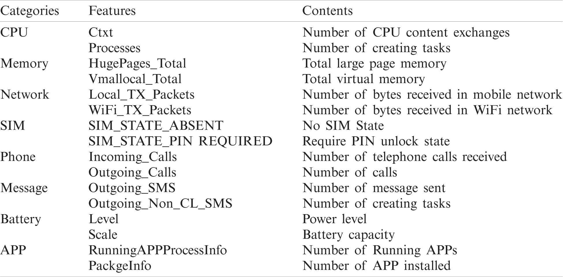
The experiment data is collected from a red mi Note1 phone, which is configured with four cores 1.6 GHz, memory 2.0 GB, and operating system MIUI8.0.1.0 (root). Normal behaviors are collected from the user’s daily behavior, such as normal use of phones and its apps. Anomaly behaviors are mainly collected from the virus behaviors of Android Malware Genome Project APK samples [16] and KaFan forum APK samples [17] in the specific period. We selected useful features by referring to three literatures [18–20]. And as a result of the Android platform version change, some new features have been added; the data contains 106 features, mainly divided into 8 categories: CPU, memory, network, SIM, phone, SMS, battery, app, etc. Some features are listed in Tab. 1. A piece of data is the cumulative value or average value over a time slice, and the time slice takes a value of 500 ms. As is shown in Tab. 1, it is part of 106 features we collected.
Table 1: The enumeration of some features
The experimental environment of this paper is DELL precision T1700 workstation, the main parameters are Inter Xeon CPU E3-1220 v3@3.10 GHz, 8 GB RAM, and the operating system is Windows 7 Ultimate. The algorithm is implemented by python 3.6. The PCA dimension reduction is implemented by PCA library function in the package of sklearn.decomposition.
In order to evaluate the performance of the anomaly detection algorithm, three main indicators in this paper are used as performance indicators to measure the anomaly detection model, which are defined as follows:
In the above equations, TP represents the number of correctly judging anomaly records. TN represents the number of correctly judging normal records. FP represents the number of incorrectly judging anomaly records. FN represents the number of incorrectly judging normal records. DR is the detection rate, FAR is the false alarm rate, and AC is the accuracy rate. In the application of anomaly detection, FAR is more important.
The first group of experiments is to compare the performance of our algorithm and other algorithms on mobile data. Both the original CFSFDP algorithm and our improved algorithm are basically trained by using 50000 data. And then the training data increases from 10000 to 50000 by 10000 at a time. The original algorithm is trained by rebuilding profiles. The improved algorithm is adaptively trained by self-incremental learning
As vividly shown in Fig. 5, it is the comparison between the improved algorithm and the original algorithm. There are two main aspects: Training time and the training profiles. These two aspects correspond to two kinds of problems, which need to be verified by experiments: the first is whether adaptive incremental learning can improve the speed of building the profiles, that is, whether building profiles by incremental learning is faster than rebuilding profiles or not; the second is whether the profiles built by incremental learning is basically the same as the original profiles. The first problem can be verified by the comparison experiment of training time. The second problem can be verified by the comparison experiment of the number of clustering center points. In Fig. 5a, the data size increases gradually from 10000 to 50000 by 10000 at one time. It can be seen that the training time of the improved algorithm is lower than the original algorithm. There are two reasons for this phenomenon, one is that the computation of building profiles by the improved algorithm is less than rebuilding profiles by the original algorithm; the other is that the improved algorithm compute a large number of distances in parallel. As depicted in Fig. 5b, the number of clustering center points generated by the improved algorithm is more than the number of clustering center points generated by the original algorithm. This may be caused by the strategy of our improved algorithm. For avoiding the fluctuation of detection performance, our strategy is designed to keep the original profile as much as possible. And this strategy will not merge the cluster centers, only increase the cluster centers.
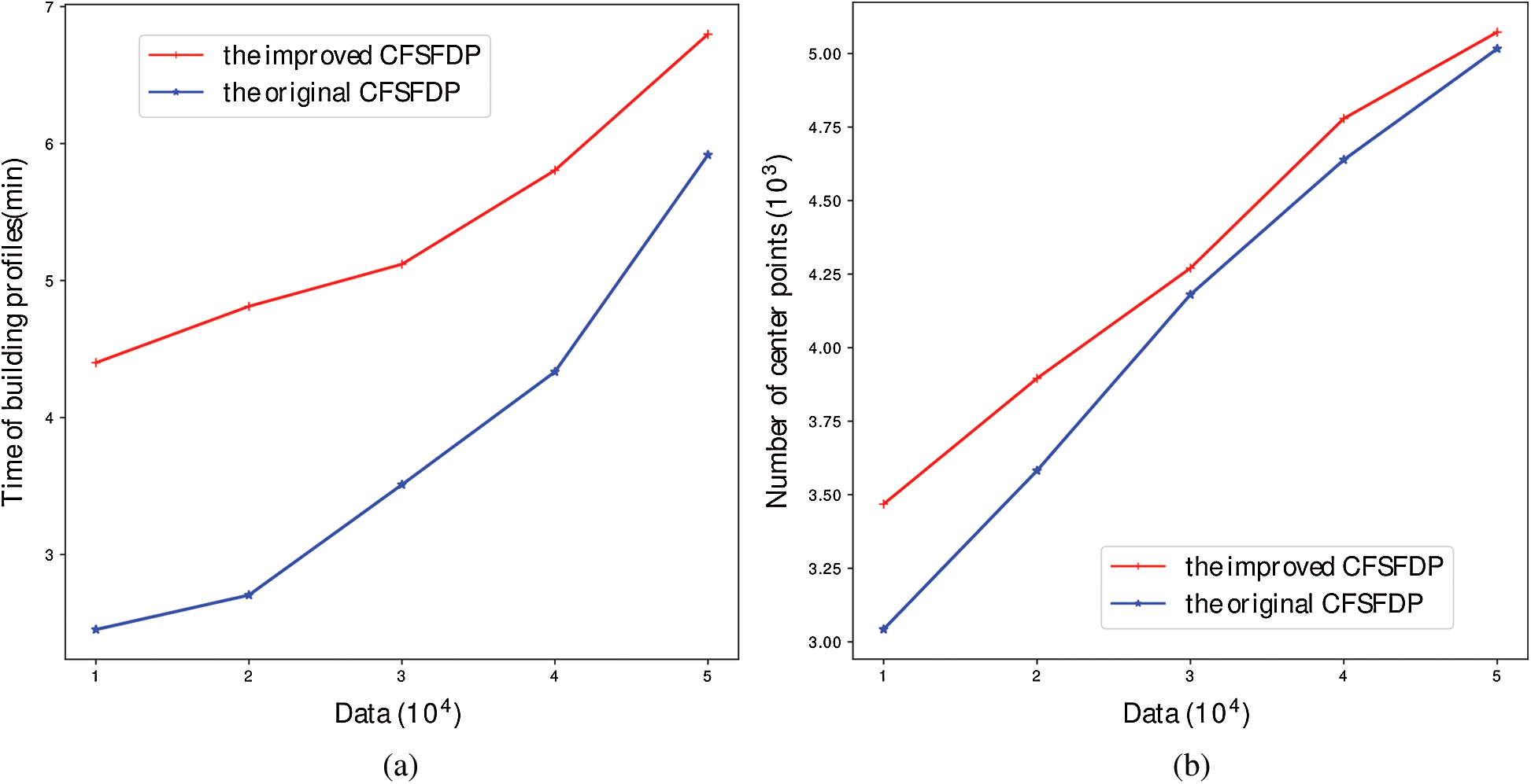
Figure 5: Performance comparison of building profiles (a) time of building profiles (b) number of center points
Detection rates of different algorithms are compared in Fig. 6a. It can be seen that ADWICE, as the classical anomaly detection algorithm, is far superior to CFSFDP and its improved algorithm, while the improved algorithm and the original algorithm have no obvious difference in detection rate. This is mainly because CFSFDP algorithm as a new anomaly detection algorithm, lack of the improvement for applying in anomaly detection, the profiles of normal behavior is not as accurate as ADWICE. In Fig. 6b, false alarm rates of different algorithms are compared. In the process of data size increment from 10000 to 20000, the false alarm rate of the improved algorithm is lower than that of the original algorithm. When incremental data size is more than 30000, the false alarm rate of the improved algorithm is higher than that of the original algorithm. The reason for this phenomenon is that the profiles of the improved algorithm only increases and does not decrease, and the expansion of the profiles leads to the decrease of precision. Meanwhile, ADWICE has the lowest false alarm rate.
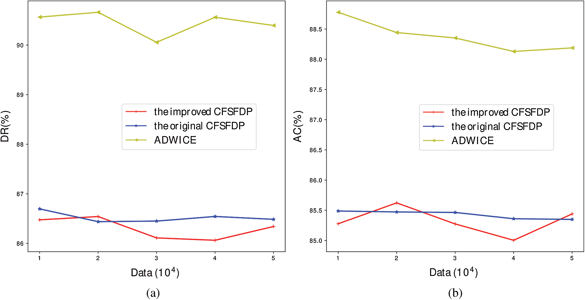
Figure 6: Performance comparison of detecting anomalies (a) time of building profiles (b) number of center points
Fig. 7 illustrates the accuracy of different algorithms under different quantities. It can be seen that ADWICE is better than CFSFDP algorithm and its derivative algorithm, and the accuracy of the improved algorithm fluctuates, while the original algorithm has been relatively stable, and the improved algorithm is not as stable as the original algorithm in terms of stability. From Figs. 6 and 7, we can see that the adaptive improvement is achieved at the expense of the stability of some algorithms.
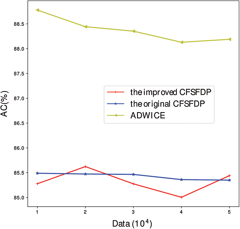
Figure 7: AC comparison of different data sizes
As we can see in Fig. 8, it is a detection rate comparison between the full feature dimensions and the partial feature dimensions. By PCA methods, the full 106 dimensions are reduced to 34 dimensions. It can be seen that the reduction of dimensions does not lead to a significant reduction in detection rates. In addition, ADWICE has the best detection rate in the full dimensions or the partial dimensions.
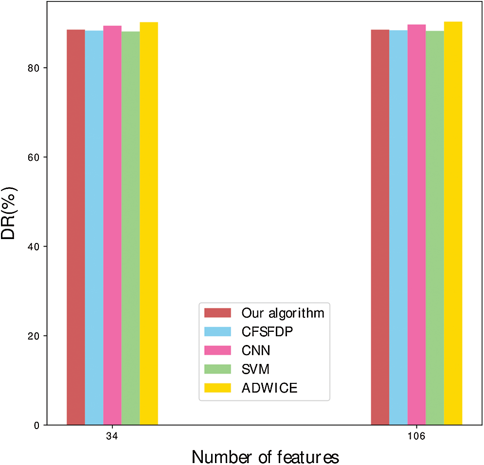
Figure 8: DR comparison of different algorithms
Obviously in Fig. 9, it is a false alarm rate comparison between the full feature dimensions and the partial feature dimensions. It can be seen that the improved algorithm has a higher false alarm rate than the original algorithm in 34 dimensions, and the improved algorithm has a lower false alarm rate than the original algorithm in 106 dimensions. In the 34 or 106 dimensions, ADWICE has the lowest false alarm rate, and the CNN has the highest false alarm rate. For anomaly detection, false alarm rate is an important performance indicator. Combined with detection rate and false alarm rate, the overall performance of the improved algorithm is good.
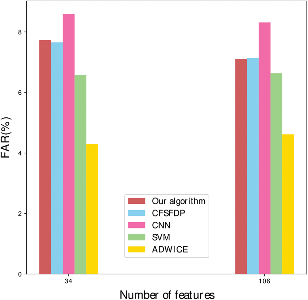
Figure 9: FAR comparison of different algorithms
Apparently in Fig. 10, there is an accuracy rate comparison between the full feature dimensions and the partial feature dimensions. The improved algorithm has lower accuracy rate than the original algorithm in 34 or 106 dimensions. The improved algorithm in 34 dimensions has the lower accuracy rate than that in 106 dimensions. Compared with other algorithms, the improved algorithm has lowest accuracy rate.
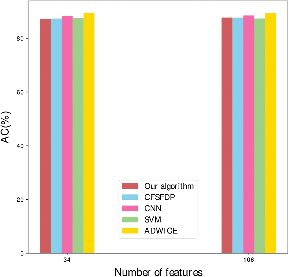
Figure 10: AC comparison of different algorithms
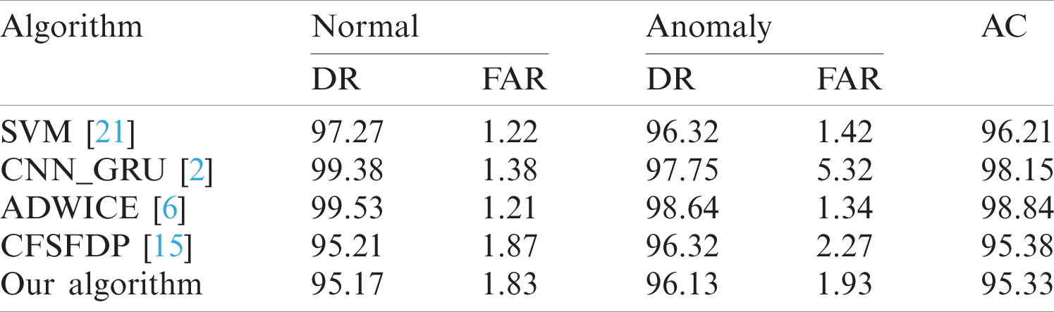
Tab. 2 is a comparison of detection performance of different algorithms using the open data set KDDCUP 1999. It is pretty easy to tell that ADWICE has a great advantage in the classic data set. Compared with other algorithms, CFSFDP and its improved algorithm do not have any advantage in accuracy, but the profiles stability of the algorithm is better when judging normal behavior and anomaly behavior.
Table 2: Detection performance comparison using KDDCUP 1999
In this paper, we propose an adaptive anomaly detection algorithm based on CFSFDP, the algorithm can learn the incremental data adaptively without changing the original profiles. It can not only avoid rebuilding profiles, but also reduce the computation and computing time. However, the strategy of the improved algorithm is not to modify the existing profiles, so the number of cluster center point only increases but not decreases. By the experimental analysis, it can be seen that the improved algorithm is to obtain the adaptability at the expense of the stability of original algorithm. In addition, the improved algorithm fail to improve the detection performance, even in some cases, the detection performance may decline. The next work will focus on two aspects: (1) the anomaly detection based on CFSFDP needs to be further improved for higher detection performance; (2) the stability of the adaptive anomaly detection based on CFSFDP needs to be further improved.
Funding Statement: This work was supported in part by the National Key Research and Development Program of China under Grant No. 2018YFB1800303, the Science and Technology Planning Project of Jilin Province under Grant No. 20190302070GX, and the Science and Technology Projects of Jilin Provincial Education Department (the 13th five year plan) under Grant Nos. JJKH20190593KJ, JJKH20190546KJ, and JJKH20200795KJ.
Conflicts of Interest: The authors declare that they have no conflicts of interest to report regarding the present study.
1. N. Shone, T. N. Ngoc, V. D. Phai and Q. Shi, “A deep learning approach to network intrusion detection,” IEEE Transactions on Emerging Topics in Computational Intelligence, vol. 2, no. 1, pp. 41–50, 2018. [Google Scholar]
2. A. Chawla, B. Lee, S. Fallon and P. Jacob, “Host based intrusion detection system with combined CNN/RNN model,” in Proc. ECML PKDD, Dublin, IE, pp. 149–158, 2018. [Google Scholar]
3. K. Alrawashdeh and C. Purdy, “Toward an online anomaly intrusion detection system based on deep learning,” in Proc. ICMLA, Anaheim, CA, USA, pp. 195–200, 2016. [Google Scholar]
4. H. Bäcklund, A. Hedblom, and N. Neijman, “A density-based spatial clustering of application with noise,” in Data Mining TNM033, Linköpings, SWE: Linköpings University, pp. 11–30, 2011. [Online]. Available: http://webstaff.itn.liu.se/~aidvi/courses/06/dm/Seminars2011/DBSCAN(4).pdf. [Google Scholar]
5. S. Shamshirband, A. Aminic, N. B. Anuar, M. Laiha and M. Kiah, “A density-based fuzzy imperialist competitive clustering algorithm for intrusion detection in wireless sensor networks,” Measurement, vol. 55, no. 9, pp. 212–226, 2014. [Google Scholar]
6. B. Kalle and S. Nadjm-Tehrani, “Adaptive real-time anomaly detection with incremental clustering,” Information Security Technical Report, vol. 12, no. 1, pp. 56–67, 2007. [Google Scholar]
7. S. Gargand and S. Batra, “A novel ensembled technique for anomaly detection,” International Journal of Communication Systems, vol. 30, no. 11, pp. e3248, 2016. [Google Scholar]
8. Y. Gu, Y. Wang, Z. Yang, F. Xiong and Y. Gao, “Multiple-features-based semisupervised clustering DDoS detection method,” Mathematical Problems in Engineering, vol. 2017, pp. 1–10, 2017. [Google Scholar]
9. R. Velea, C. Ciobanu, L. Mrgrit and I. Bica, “Network traffic anomaly detection using shallow packet inspection and parallel K-means data clustering,” Studies in Informatics and Control, vol. 26, no. 4, pp. 387–398, 2017. [Google Scholar]
10. J. Zou, D. Tao and J. Yu, “A hybrid intrusion detection model for web log-based attacks,” Journal of Internet Technology, vol. 18, no. 4, pp. 886–895, 2017. [Google Scholar]
11. J. Dromard, G. Roudière and P. Owezarski, “Online and scalable unsupervised network anomaly detection method,” International Journal of Interactive Multimedia and Artificial Intelligence, vol. 4, no. 6, pp. 54–59, 2017. [Google Scholar]
12. J. Karimpour and S. Lotfi, “Intrusion detection in network flows based on an optimized clustering criterion,” Turkish Journal of Electrical Engineering and Computer Sciences, vol. 25, no. 3, pp. 1963–1975, 2017. [Google Scholar]
13. S. H. Oh and W. S. Lee, “An anomaly intrusion detection method by clustering normal user behavior,” Computers & Security, vol. 22, no. 7, pp. 596–612, 2003. [Google Scholar]
14. A. Rodriguez and A. Laio, “Clustering by fast search and find of density peaks,” Science, vol. 344, no. 6191, pp. 1492–1496, 2014. [Google Scholar]
15. W. Ren, J. Zhang, X. Di, Y. Lu, B. Zhang et al., “Anomaly detection algorithm based on CFSFDP,” Journal of Advanced Computational Intelligence and Intelligent Informatics, vol. 24, no. 4, pp. 453–460, 2020. [Google Scholar]
16. Y. Zhou and X. Jiang, “Android malware genome project,” 2018. [Online]. Available: http://www.malge-nomeproject.org. [Google Scholar]
17. Kaspersky Fans, “Virus sample area,” 2018. [Online]. Available: https://bbs.kafan.cn/thread1671514-1-1.html. [Google Scholar]
18. I. Burguera, U. Zurutuza and S. N.Tehrani, “Crowdroid: Behavior-based malware detection system for Android,” in Proc. SPSM, NY, USA, pp. 15–26, 2011. [Google Scholar]
19. A. Reina, A. Fattori and L. Cavallaro, “A system call-centric analysis and stimulation technique to automatically reconstruct android malware behaviors,” in Proc. EuroSec, Prague, CZ, 2013. [Google Scholar]
20. A. Shabtai, U. Kanonov, Y. Elovici, C. Glezer and Y. Weiss, “A behavioral malware detection framework for Android devices,” Journal of Intelligent Information Systems, vol. 38, no. 1, pp. 161–190, 2011. [Google Scholar]
21. D. Zhang, F. Ren, K. Zhao, Y. Zhang and X. Liu, “An online unsupervised intrusion detection system based on SVM,” Journal of Jilin University, vol. 47, no. 2, pp. 323–329, 2009. [Google Scholar]
 | This work is licensed under a Creative Commons Attribution 4.0 International License, which permits unrestricted use, distribution, and reproduction in any medium, provided the original work is properly cited. |