DOI:10.32604/cmc.2021.016732
| Computers, Materials & Continua DOI:10.32604/cmc.2021.016732 | |
| Article |
Estimating Age in Short Utterances Based on Multi-Class Classification Approach
1College of Managerial and Financial Sciences, Imam Ja’afar Al-Sadiq University, Salahaddin, Iraq
2Department of Computer Science, University of Technology, Baghdad, Iraq
*Corresponding Author: Ameer A. Badr. Email: cs.19.53@grad.uotechnology.edu.iq
Received: 07 January 2021; Accepted: 10 February 2021
Abstract: Age estimation in short speech utterances finds many applications in daily life like human-robot interaction, custom call routing, targeted marketing, user-profiling, etc. Despite the comprehensive studies carried out to extract descriptive features, the estimation errors (i.e. years) are still high. In this study, an automatic system is proposed to estimate age in short speech utterances without depending on the text as well as the speaker. Firstly, four groups of features are extracted from each utterance frame using hybrid techniques and methods. After that, 10 statistical functionals are measured for each extracted feature dimension. Then, the extracted feature dimensions are normalized and reduced using the Quantile method and the Linear Discriminant Analysis (LDA) method, respectively. Finally, the speaker’s age is estimated based on a multi-class classification approach by using the Extreme Gradient Boosting (XGBoost) classifier. Experiments have been carried out on the TIMIT dataset to measure the performance of the proposed system. The Mean Absolute Error (MAE) of the suggested system is 4.68 years, and 4.98 years, the Root Mean Square Error (RMSE) is 8.05 and 6.97, respectively, for female and male speakers. The results show a clear relative improvement in terms of MAE up to 28% and 10% for female and male speakers, respectively, in comparison to related works that utilized the TIMIT dataset.
Keywords: Speaker age estimation; XGBoost; statistical functionals; Quantile normalization; LDA; TIMIT dataset
The speech contains valuable linguistic context information and paralinguistic information about speakers, such as identity, emotional state, gender, and age [1]. Automatic recognition of this kind of information can guide Human-Computer Interaction (HCI) systems to adapt in an automatic way for various user needs [2].
Automatic age estimation from short speech signals has a variety of forensic and commercial applications. It may be used in several forensic scenarios like threat calls, kidnapping, and falsified alarms to help identify criminals, e.g., shorten the number of suspects. Automatic age estimation may also be used for effective diverting of calls in the call centers [1–3].
Estimating the age of the speaker is a difficult estimation issue for several reasons. First, the age of the speaker is a continuous variable, which makes it difficult to be estimated by algorithms of machine learning that are working with discrete labels. Second, there is usually a difference between a speaker’s age as perceived, namely the perceptual age, and their actual age, that is, the chronological age. Third, there are very few publicly available aged labeled datasets with a sufficient number of speech utterances for various age groups. Finally, the speakers of the same age may sound different due to the intra-age variability such as speaking style, gender, weight, speech content, height, emotional state, and so on [1–4].
The TIMIT speech reading corpus has been designed for providing speech data for the acoustic-phonetic studies and for developing and evaluate the systems of automatic speech recognition. TIMIT includes broadband recordings of 630 speakers of 8 main American English dialects; every one of them reads 10 phonetically rich sentences. Recently, some studies are interested in studying the age estimation system based on the TIMIT dataset. Singh et al. [5] proposed an approach to estimating speakers’ psychometric parameters such as height and age. They stated that when analyzing the signal at a finer temporal resolution, it may be possible to analyze segments of the speech signal that are obtained entirely when the glottis is opened and thereby capturing some of the sub-glottal structure that may be represented in the voice. They used a simple bag-of-words representation together with random forest regression to make their predictions. For age estimation, the Mean Absolute Error (MAE) of their best results was 6.5 and 5.5 for female and male speakers, respectively. Kalluri et al. [6] proposed an end-to-end architecture for the prediction of the height as well as the age of the speaker based on the Deep Neural Networks (DNNs) for short durations of speech. For age estimation, the Root Mean Square Error (RMSE) of their best results was 8.63 and 7.60 for female and male speakers, respectively. Kalluri et al. [7] explored, in a multilingual setting, the estimation of the speaker’s multiple physical parameters from a short speech duration. At different resolutions, they used various feature streams for the estimation of the body-build and age that have been derived from the spectrum of the speech. To learn a Support Vector Regression (SVR) model for the estimation of the speaker body-build and age, the statistics of these features are used over speech recording. For age estimation, the MAE of their best results was 5.6 and 5.2, respectively, for female and male speakers.
The previous studies conducted a variety of different methods and techniques such as random forest regression, DNN, and SVR to estimate age from short speech utterances accurately. However, the prediction errors (i.e., years) are still high for real-time applications like human-robot interaction. The reason behind this is their inability to efficiently find the combination of features that characterize the speaker’s age; they use a sort of old estimation techniques. The main objective of this study is to build an accurate speaker age estimator that bridges the gap of an appropriate combination of features by finding the optimal feature vectors that depend on statistical functionals as well as the LDA method to make the prediction errors as small as possible.
The primary contributions of the present study can be highlighted and summarized as follows:
1. Combining four feature groups, which are Mel-Frequency Cepstral Coefficients (MFCCs), Spectral Subband Centroids (SSCs), Linear Predictive Coefficients (LPCs), and Formants to extract 150-dimensional feature vectors from each utterance.
2. Measuring 10 statistical functionals for each extracted feature dimension to achieve the greatest possible gain from each feature vector.
3. Exploring the role of using the Quantile technique as a feature normalization method.
4. Exploring the role of using Linear Discriminant Analysis (LDA) as a supervised approach for dimensionality reduction.
5. Treating the age estimation issue as a multi-class classification issue by using the XGBoost classifier to predict the speaker’s age from short utterances.
The rest of this study is organized as follows: Section 2 presents the theoretical backgrounds of the proposed system. Section 3 deals with the proposed method. The results of simulations and experiments are shown in Section 4. Finally, Section 5 sets out the study conclusions and future works.
In the present study, several methods and techniques were used to extract the features from each speech utterance, reduce the extracted features dimensionality, and estimate speaker age. These methods and techniques are described briefly below.
2.1 Features Extraction Methods
As mentioned before, the speech signal contains various types of paralinguistic information, e.g., speaker age. Features are determined at the first stage of all classification or regression systems, where the speech signal is transformed into measured values with distinguishing characteristics. Such methods used in this study are briefly described below.
2.1.1 The Mel-Frequency Cepstral Coefficients (MFCCs)
Among all types of speech-based feature extraction domains, Cepstral domain features are the most successful ones, where a cepstrum has been obtained by taking the inverse Fourier transform of the signal spectrum. MFCC is the most important method to extract speech-based features in this domain [8,9]. MFCCs magnificent role stems from the ability to exemplify the spectrum of speech amplitude in a concise form. The voice of the speaker is filtered by the articulator form of the vocal tract, like the nasal cavity, teeth, and tongue. This shape affects the vibrational characteristics of the voice. If the shape is precisely controlled, this should give an accurate depiction of the phoneme being formed [10]. The procedure for obtaining the MFCC features are shown in Fig. 1 [11] and the following steps [12]:
1) Preemphasis: This relates to the filtering, which stresses the higher frequency values. It aims to offset the range of voiced sounds that are in the high-frequency area have a steep roll-off. Therefore, some of the glottal effects are eliminated from the parameters of the vocal tract by preemphasis.
2) Frame blocking and windowing: Speech must be examined over a short period of time (i.e., frames) for stable acoustic characteristics. A window is applied on each frame for tapering the signal toward the limits of the frame. Hamming windows are usually used.
3) FFT spectrum: By applying the Fast Fourier Transform (FFT), every one of the windowed frames has been converted to a spectrum of magnitude.
4) Mel spectrum: By passing the FFT signal through a set of the bandpass filters referred to as Mel-filter bank, a Mel spectrum is computed. A Mel is a measurement unit that has been based upon the perceived frequency of the human ear. The Mel scale is approximately below 1 kHz linear frequency spacing and above 1 kHz logarithmic spacing. It is possible to express the Mel approximation from the physical frequency as in Eq. (1). The warped axis, based on the non-linear function that has been given in Eq. (1), has been implemented to mimic the perception of human ears. The filter shaper most commonly used is triangular. Through multiplying the spectrum magnitude by every triangular Mel weighting filter, the Mel of magnitude spectrum X (k) has been calculated as expressed in Eq. (2).

Figure 1: The MFCC analysis process [11]
where fMel is the perceived frequency in Hz, and f is the physical frequency. M is the total number of triangular Mel weighting filters, Hm(k) is the kth energy spectrum bin weight contributing to mth output band.
5) Discrete cosine transform (DCT): The levels of the energy in the adjacent bands have the tendency of being correlated since the vocal tract is smooth. A set of cepstral coefficients is produced by the DCT applied to the coefficients of the transformed Mel frequency. Finally, MFCC is calculated as expressed in Eq. (3).
where c(n) is the cepstral coefficients, and C represents the number of the MFCCs.
6) Dynamic MFCC features: The additional information on the time dynamics of a signal is obtained by computation of the cepstral coefficients’ first and second derivatives since they contain only information from the given frame. Eq. (4) show the commonly utilized definition for the computation of the dynamic parameter.
where
2.1.2 Spectral Subband Centroids (SSCs)
SSC feature proposed by Paliwal [13] is intended to be a complement to the cepstral features in speech recognition. High sensitivity to additive noise distortion is considered as a major problem concerning the cepstral-based features, the addition of the white noise to the speech signals affects the spectrum of speech power at all frequencies, but in the higher amplitude (formant) portions of the spectrum, the effect is less noticeable. Therefore, to ensure the robustness of the feature, some formant-like features have to be investigated; SSC features are similar to the formant frequencies and can be easily and reliably extracted [13]. The entire frequency band (0 to Fs/2) has been divided into N number of sub-bands for computation of SSCs, where Fs is the speech signal sampling frequency. SSCs are found through the application of the filter banks to the signal power spectrum and, after that, the calculation of the first moment (i.e., centroid) of every one of the sub-bands. SSC of mth subband is calculated as seen in Eq. (5), where Fs is the frequency of sampling,
2.1.3 Linear Predictive Coefficients (LPCs)
LPCs are techniques developed to analyze speech. The idea behind this is to model the production of speech as an additive model consisting of a source and a filter with one or more resonant frequencies. The source corresponds to the vocal folds’ primary vibrations, and the filter is due to the vocal tracts’ shapes and movements, that is, the throat, the tongue, and the lips [15]. By predicting a formant, LPC analysis decided on a signal format, which is referred to as the inverse filtering, after that, estimated the frequency and intensity from the residue speech signal. Due to the fact that the speech signal has numerous time-dependent types, the estimate will cut a signal that is referred to as a frame. The process for obtaining the LPC coefficient is illustrated in Fig. 2 and the following steps [16]:
1) Preemphasis: This relates to filtering, which stresses the higher frequency levels. It aims to offset the range of voiced sounds that in the high-frequency area have a steep roll-off. As expressed in Eq. (6), the Preemphasis filter is based on the time-domain input/ output relation.
2) Frame blocking and windowing: Speech should be examined over a short period of time (i.e., frames) for stable acoustic characteristics. A window is applied on each frame for tapering the signal toward the limits of the frame. Hamming windows w(n) are usually used as expressed in Eq. (7).
3) Autocorrelation Analysis: in this step, autocorrelation analysis is implemented toward each frame result by Eq. (7), as expressed in Eq. (8).
where p denotes the LPC order that is often from (8) to (16).
4) LPC Analysis: every one of the frames from the autocorrelation of (p + 1) is converted in this step to become a compilation of LPC parameters. This compilation then becomes an LPC coefficient or becomes a transformation of another LPC. The formal method to do that is called the Durbin method.
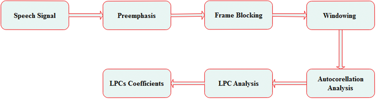
Figure 2: The LPC process [16]
The vocal tract shape includes a lot of the relevant information, and it was commonly represented in numerous applications that are associated with the speech. The formants, a vocal tract resonance representation, may be modeled with the LPC [17]. The formants are merely spectral spectrum peaks of the voice. In the phonetics of the speech, the formant frequency levels are the acoustic resonance of the human vocal tract, which is measured as a peak of the amplitude in the sound frequency spectrum. In acoustics, formants are known as a peak in the sound envelope and/or the resonance in sound sources, in addition to sound chambers. The process for getting the formant features is shown in Fig. 3 [18].

Figure 3: The formants detection process [18]
2.2 Quantile Normalization Method
There are numerous normalization techniques used with machine learning algorithms such as min–max transformation, z-score transformation, and power transformation. Among them, Quantile normalization was originally developed for gene expression microarrays, but today it is applied in a wide range of data types. Quantile normalization is a global method of adjustment that assumes that each sample’s statistical distribution is the same. The method is supported by the concept that a quantile–quantile plot indicates that if a plot is a straight diagonal line, the distribution of two data vectors is the same, and not the same, if it is different from a diagonal line. This definition is extended to N-dimensions; therefore, in the case where every N data vector has an identical distribution to the others, then plotting the quantiles in N-dimensions provides a straight line along the unit vector line. This indicates that if one projects the points of our N-dimensional quantile plot onto the diagonal, one could create a set of data with the same distribution. This implies that an identical distribution may be given to every one of the arrays by taking the average quantile and substituting it as the data item value in the original dataset [19,20]. This results in motivating the following steps by giving them the same distribution to normalize a set of data vectors [19]:
1. Given n arrays of length p, form X of dimension
2. Sorting every one of the columns of X to result in Xsort;
3. Taking the mean values across the rows of Xsort and assigning that mean to every one of the elements in a row to obtain
4. Getting
2.3 Linear Discriminate Analysis (LDA) Method
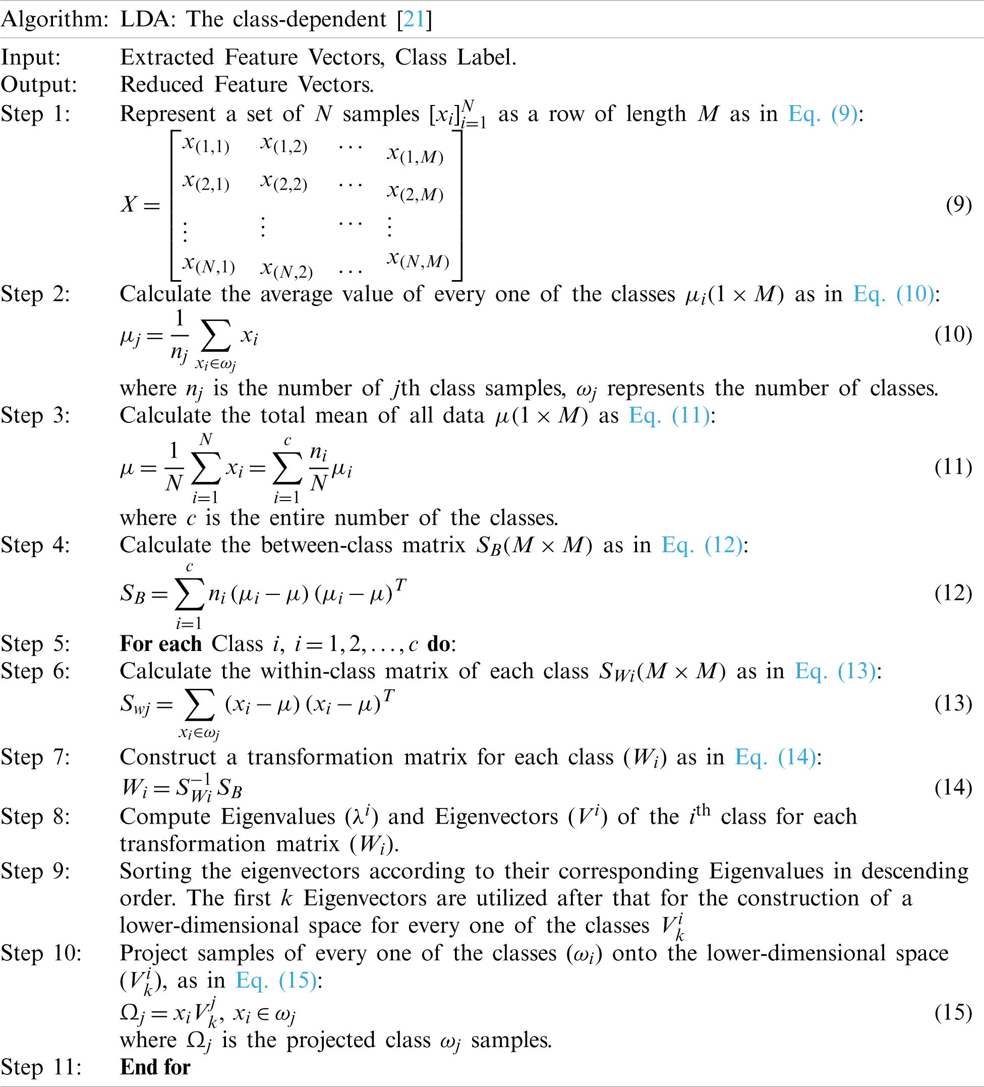
Mainly, there is a degree of redundancy in extracted high-dimensional characteristics. Sub-space learning may be utilized for the elimination of those redundancies through the additional processing of the obtained features for the purpose of reflecting their semantic information in a sufficient way. There are numerous dimensionality reduction techniques used with machine learning algorithms such as Principal Component Analysis (PCA), Non-negative Matrix Factorization (NMF), and, Factor Analysis. Among them, LDA is one of the very common supervised techniques for the problems of dimensionality reduction as a preprocessing step for applications of pattern classification and machine learning. The LDA technique aims at projecting the original data matrix in a lower-dimensional space. There have been three steps required for achieving that goal. The initial step is calculating the variance amongst classes (in other words, the distance between the mean values of various classes). The second step is to calculate the within-class variance, which is the distance between the mean and the samples of every one of the classes. The third step is the construction of the lower-dimensional space, which minimizes the within-class variance and maximizes the between-class variance [21]. Tab. 1 illustrates the main steps of the supervised LDA algorithm.
Table 1: The class-dependent LDA
2.4 Extreme Gradient Boosting Machine (XGBoost)
Based on the ensemble boosting idea, the XGBoost is combining all sets of weak learner’s predictions through additive training strategies to develop a strong learner. The XGBoost seeks to avoid over-fitting beside optimize the computing resources. This is accomplished by modeling the objective functions, allowing regularization and predictive terms to be combined but also maintain an optimum computation speed. During the XGBoost phase training, parallel calculations are performed automatically for each function [22].
In the learning process of the XGBoost, the first learner is fitted to the entire input data space, while a second model is to tackle the drawbacks of a weak learner by fitted to residuals. Until the stopping criterion has been met, this fitting process will be repeated a number of times. The model’s final prediction is obtained by the sum of each learner’s prediction. [22]. For prediction at step t, the general function has been presented as [22]:
where ft(xi) is the learner at step t,
The XGBoost model prevents overfitting issue without compromise the model computational speed by evaluating the model goodness from the original function as in the following expression [23]:
where L represents the loss function, n represents the number of the used observations, and
where
3 The Proposed Speaker Age Estimation System
As can be seen from Fig. 4, the methodology of this study consists of five main stages: features extracting, statistical functionals measuring, features normalizing, dimensionality reducing, and speaker age estimating. Initially, appropriate features are extracted from each speaker’s utterance, followed by features scaling to fall within a smaller range using normalization techniques. Then, by using the dimensionality reduction method, the high dimensional features will be transformed into more meaningful low dimensional features. Finally, an estimator based on the XGBoost classifier is used to predict the speaker’s actual age.
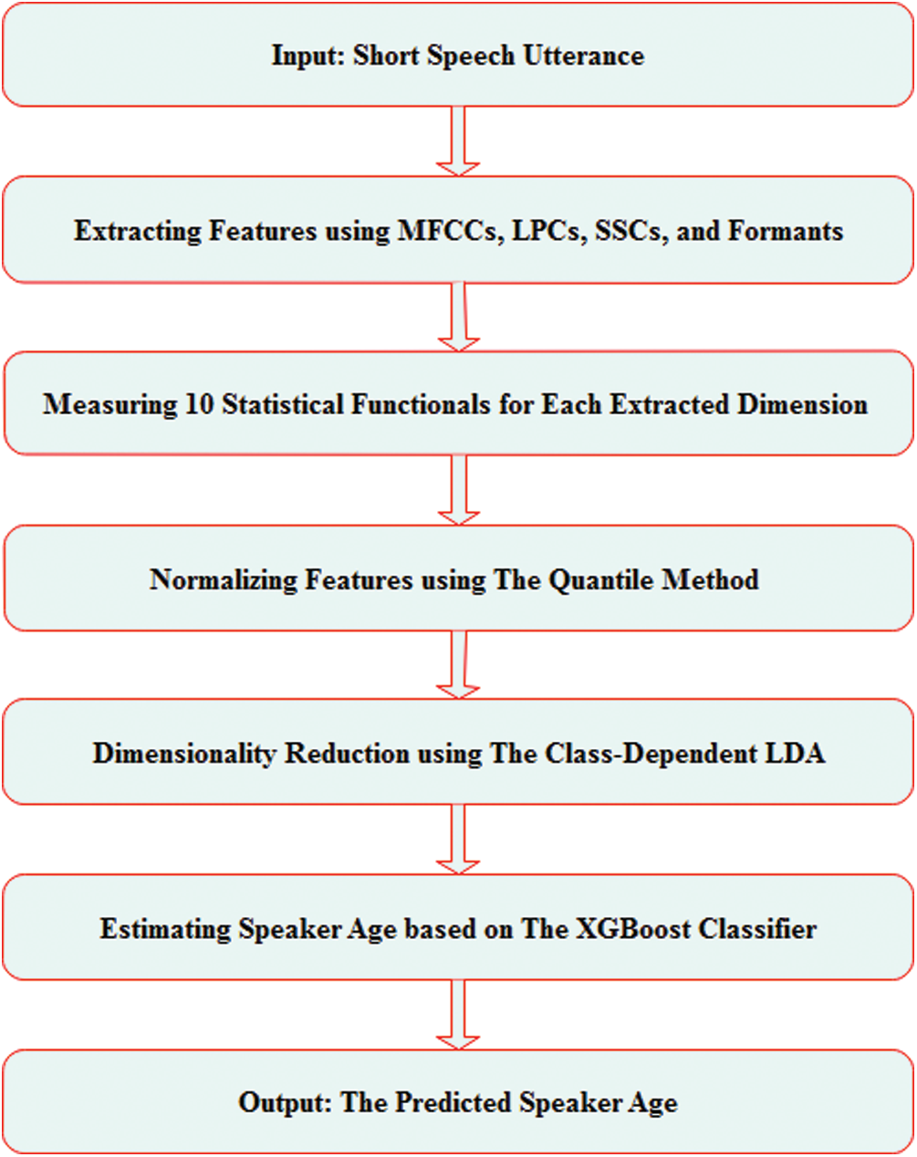
Figure 4: The general framework of the proposed system
3.1 Utterance Based Features Extraction
As mentioned earlier, the issue of estimating a speaker’s age is a difficult one where the extracted features need to be speaker-independent. Therefore, four groups of features were incorporated in this study in which the errors of the estimation from the variety of the feature groups are complementary, allowing estimates from those feature groups to be combined to additionally enhance system performance. In the beginning, each speaker’s utterance is split into frames with a window size of 250 milliseconds and a frameshift of 10 milliseconds to ensure that each frame contains robust information. Then, four groups of features are extracted from each utterance frame, which are MFCC (i.e., 20-dimensions with its first and second derivative), LPC (i.e., 20-dimensions with its first and second derivative), SSC (i.e., 26-dimension), and formants (i.e., F1, F2, F3, and F4.). The total dimensions of the extracted features in this stage are 150, as seen in Fig. 5.
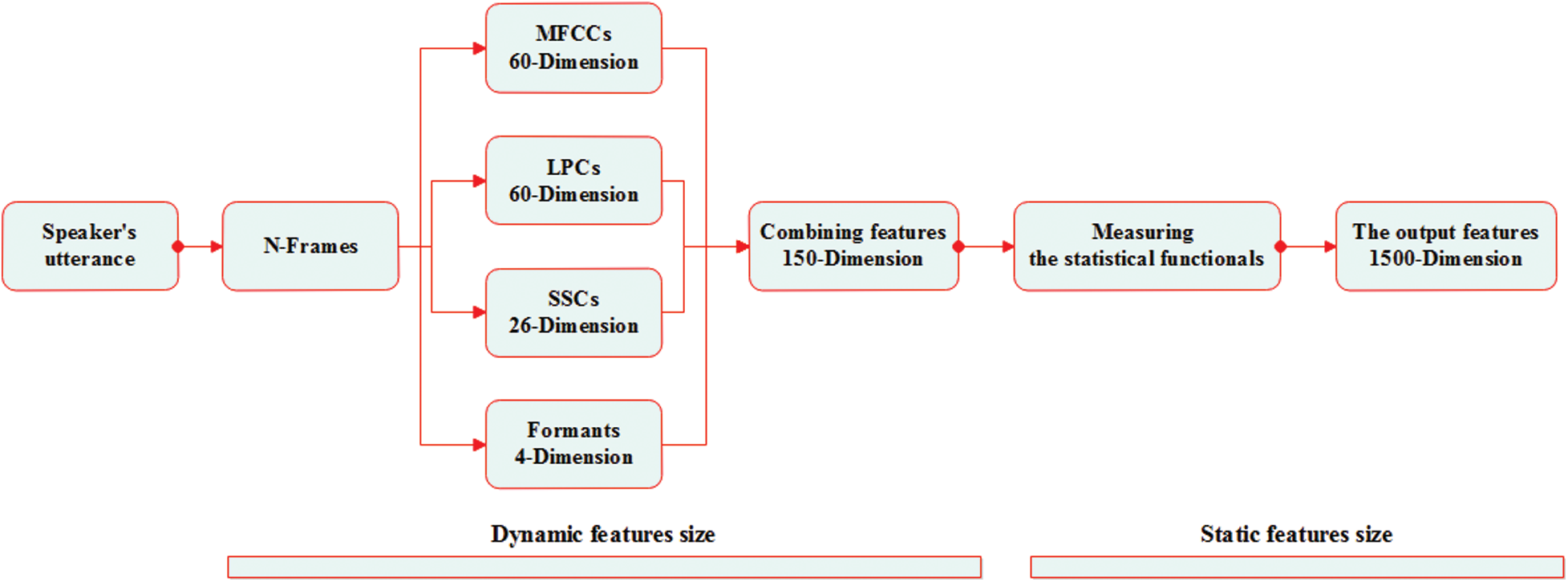
Figure 5: The proposed features fusion
3.2 Statistical Features Generation
To override the issue of varying features size between different speaker utterances as well as to achieve the greatest possible gain from each feature dimension, the features with dynamic size extracted from the previous stage (i.e., 150-dimension) are turned into features with static size by measuring 10 statistical functionals for each dimension. These statistical functionals include mean, min, max, median, stander deviation, skewness, kurtosis, first quantile, third quantile, and interquartile range (Iqr). The total output of features dimension in this stage is 1500, as seen in Fig. 5.
3.3 Feature Normalization Using Quantile Method
The expression of features in smaller units will result in a wider range for these features and thus will tend to give such features a greater effect. The normalization process involves transforming the data to fall in a smaller range. Therefore, due to the great usefulness of the normalization process in machine learning methods, the 1500-dimensional features extracted from the previous stage will be normalized by using the quantile method.
3.4 Dimensionality Reduction Using LDA Method
At this stage, LDA takes as its input a set of 1500-dimensional normalized features grouped into labels. Then, it tends to be finding an optimum transformation mapping those input features to a lower-dimensional space at the same time as maintaining the structure of the label. Employing LDA algorithm as in Tab. 1 would maximize the between-label distance and at the same time, minimize the within-label distance, thereby achieving the maximal differentiation. The output of this stage is determined depending on Eq. (19), to produce a feature vectors containing the most important information to accurately estimate the speakers’ ages from their voice.
where NC denote the number of classes, while NF denote the number of features dimensions.
3.5 Age Estimation Using the XGBoost Classifier
In this study, the XGBoost is relied on because of its apparent superiority over most other ensemble algorithms in many respects such as parallelization, cache optimization, optimal computational speed, and curbs over-fitting easily. The XGBoost has been used recently in several speech-based applications such as Epilepsy detection [23] and Parkinson’s disease classification [24]. Age estimation is typically considered as a regression problem. However, some studies have recently treated it as a multi-class classification problem, as in Ghahremani et al. [25]. Therefore, to take advantage of the XGBoost classifier strength, the XGBoost classifier is trained on the previous stage output to estimate the speaker’s age at the minimum error rate.
4 Experimental Results and Discussions
The dataset used in this study is described, and the experiments that were performed are explained and discussed in detail in this section. Two objective measures that are utilized in the earlier studies [6,25] have been considered to evaluate the efficiency of the proposed system of age estimation.
MAE is calculated according to Eq. (20); lower MAE means better performance. RMSE is computed as in Eq. (21); lower RMSE means better performance.
where N represents the number of the test utterances,
For providing a more objective measure of comparison to the related works, the relative improvement of MAE and RMSE to the prior system is calculated as in Eqs. (22) and (23), respectively [26].
where MAE and RMSE denote the estimation error measures for the proposed system, while
The TIMIT corpus of the reading speech has been designed in order to develop and evaluate automatic speech recognition systems. Text corpus design is a joint effort amongst Stanford Research Institute (SRI), Texas Instruments (TI), and Massachusetts Institute of Technology (MIT). The speech is recorded at TI and transcribed at MIT. The sampling frequency of recoded utterances is chosen to be 16 kHz with a 16-bit rate. The duration of each utterance is about (1–3 seconds). TIMIT includes a total of 6,300 sentences, 10 sentences that are spoken by every one of the 630 speakers from 8 main dialect regions of the U.S. [27]. The statistics of the dataset are given in Tab. 2.
Table 2: TIMIT dataset statistics
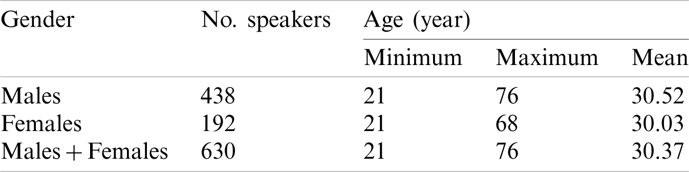
To train, test, and compare the proposed system consistently, the TIMIT dataset has been divided into two parts; the training set contains 154, and 350 speakers (i.e. 80%) while the test set contains 38, and 88 speakers (20%), respectively, for females and males. To prevent overfitting during the training process, the overlapping of speakers as well as utterances in partitioning have been avoided.
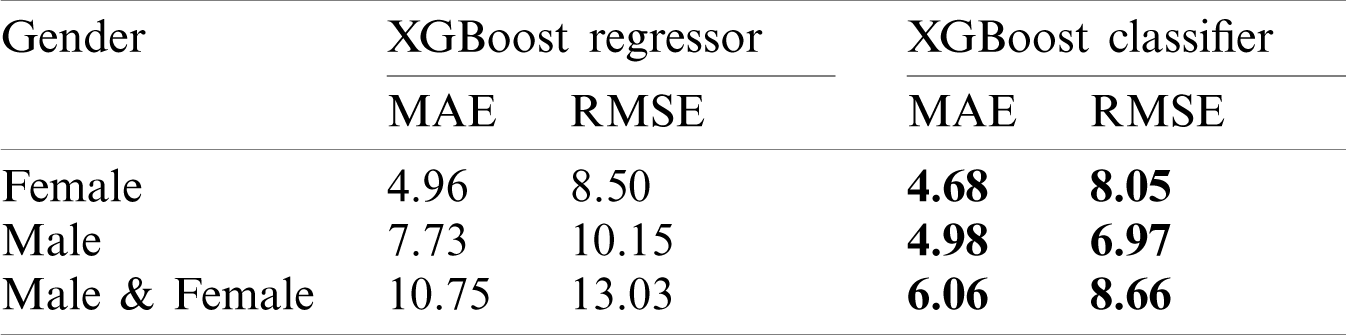
Different experiments have been carried out to find the optimal configuration of the proposed age estimation system parameters. In the first experiment, the performance evaluation of the suggested age estimation system in terms of MAE, and RMSE is conducted. Tab. 3 lists the results of this experiment. The table reports the results for both gender-dependent and gender-independent system. The table also compares the XGBoost regressor, and the XGBoost classifier results. It demonstrates the high efficiency of the XGBoost classifier over the XGBoost regressor by taking advantage of the XGBoost classifier strength when dealing with multi-class classification issues. In gender-dependent system, the MAE and RMSE metrics of the XGBoost classifier are better than the XGBoost regressor metrics for both female and male speakers, where the MAE is decreased from 4.96 as a regression output into 4.68 as a classification output in the female’s part. The MAE is also significantly decreased from 7.73 as a regression output into 4.98 as a classification output in the male’s part. On the other hand, the RMSE is significantly decreased from 8.50, 10.15 as regression outputs into 8.05, 6.97 as a classification output for female and male speakers, respectively. In gender-independent system, the MAE and RMSE metrics of the XGBoost classifier are also better than the XGBoost regressor, where the MAE and RMSE is significantly decreased from 10.75, 13.03 as a regression output into 6.06, 8.66 as a classification output, respectively. The table demonstrates the high efficiency of the proposed system in both gender-dependent and gender-independent one.
Table 3: Performance evaluation of the proposed age estimation system in terms of MAE (years), and RMSE (years) on the TIMIT dataset
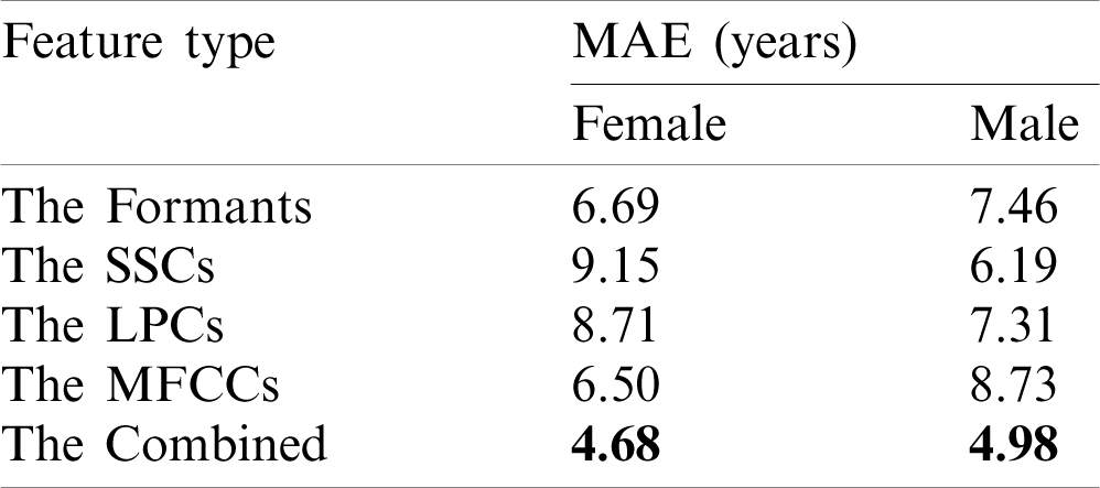
The second experiment shows the impact of each feature group on the performance of the suggested system in terms of the MAE. Tab. 4 shows the results of this experiment. The table shows the impact of each of the proposed feature groups on the efficiency of the proposed system in terms of MAE. The table demonstrates that the estimation errors from those different groups of features are complementary, allowing estimates from those feature groups to be combined to additionally enhance the results.
Table 4: The impact of each feature group on the proposed system performance in terms of MAE on the TIMIT dataset
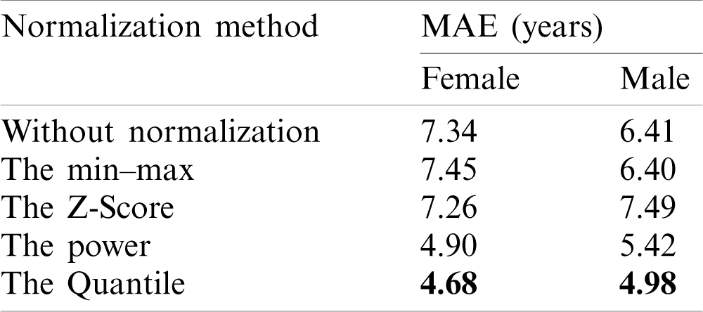
The third experiment compares the proposed normalization method (i.e., quantile) with other normalization methods in terms of MAE. Tab. 5 shows the results of this experiment. The table shows a comparison in terms of MAE between the proposed normalization method, which is a quantile, and three other baseline methods, which are min–max transformation, z-score transformation, and power transformation, in addition to without normalization case. The table demonstrates that implementing the proposed Quantile normalization method presents better performance (i.e., lower MAE) because the Quantile transformation method tends to spread out the most frequent values which therefore reduced the impact of outliers.
Table 5: Comparison in terms of MAE (years) between the proposed normalization method and other normalization methods on the TIMIT dataset
The fourth experiment compares the proposed dimensionality reduction method (i.e., LDA) with other dimensionality reduction methods in terms of MAE. Tab. 6 shows the results of this experiment. The table shows a comparison in terms of MAE between the proposed dimensionality reduction method, which is the LDA and three other baseline methods which are PCA NMF, and, Factor Analysis, in addition to without reduction case. The table demonstrates that implementing the LDA method presents a significantly better performance (i.e., lower MAE) because the LDA method reduces the dimensions depending on the class-label (i.e., supervised reduction).
Table 6: Comparison in terms of MAE (years) between the proposed dimensionality reduction method and other dimensionality reduction methods on the TIMIT dataset

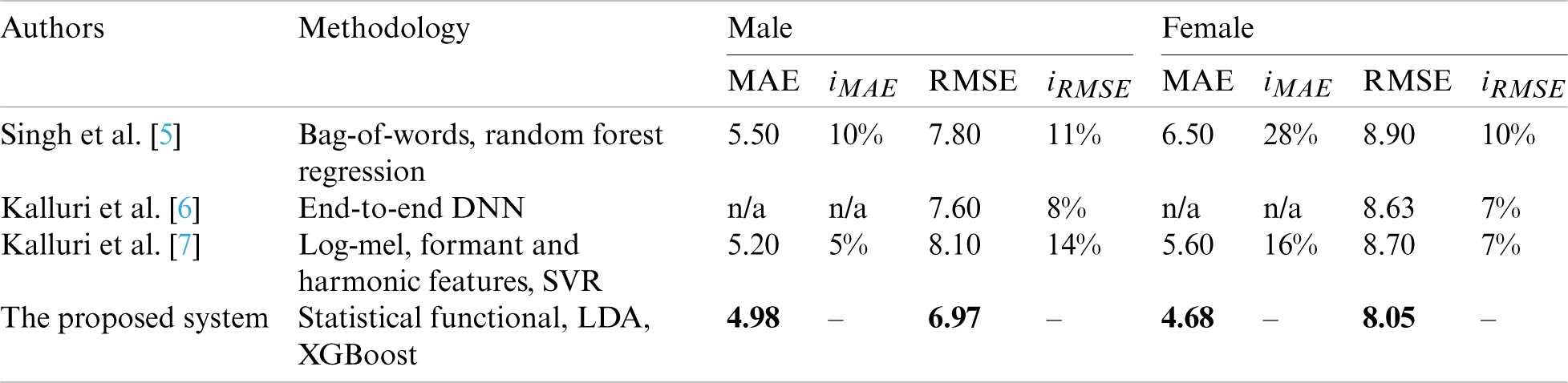
Finally, a comparison of the proposed system with related works utilizing the same dataset (i.e., TIMIT dataset) in terms of MAE and RMSE is presented in the fifth experiment. Tab. 7 shows the results of this experiment. In the case of MAE, the relative improvement (iMAE) of the proposed system is up to 10% and 28% for male and female speakers, respectively. In the case of RMSE, the relative improvement (iRMSE) of the proposed system is up to 14% and 10% respectively for male and female speakers. The table demonstrates the superiority of the proposed system taking advantage of using features fusion, statistical functionals, supervised LDA, and XGBoost classifier.
Table 7: Comparison in terms of the MAE (years) and RMSE (years) between the proposed system and related works which are utilized the TIMIT dataset
An automatic system to estimate age in short speech utterances without depending on the text as well as the speaker is proposed in this study. Four groups of features are combined to further improve system performance. Then, the dynamic size features are turned into static size features by measuring 10 statistical functionals for each dimension. After that, the use of the LDA method has a major impact on the efficiency of the system by producing a reduced informative feature vector. Finally, the proposed system treating the age estimation problem as a multi-class classification problem taking advantage of the XGBoost classifier strength. The experimental results clearly show the effectiveness of the proposed system in both gender-dependent and gender-independent with MAE of 4.68, 4.98, and 6.06 for female, male, and male & female speakers, respectively, using the TIMIT dataset. For future work, a DNN may be utilized for joint gender and age estimation from short utterances where the network can be fed with the same reduced feature vectors proposed in this study.
Funding Statement: The authors received no specific funding for this study.
Conflicts of Interest: The authors declare that they have no conflict of interest to report regarding the present study.
1. P. G. Shivakumar, M. Li, V. Dhandhania and S. S. Narayanan, “Simplified and supervised i-vector modeling for speaker age regression,” in Proc. IEEE Int. Conf. on Acoustics, Speech, and Signal Processing, Florence, Italy, pp. 4833–4837, 2014. [Google Scholar]
2. M. Li, C. S. Jung and K. J. Han, “Combining five acoustic level modeling methods for automatic speaker age and gender recognition,” in Proc. 11th Annual Conf. of the Int. Speech Communication Association, Makuhari, Chiba, Japan, pp. 2826–2829, 2010. [Google Scholar]
3. M. H. Bahari, M. McLaren, H. Van-Hamme and D. A. Van-Leeuwen, “Speaker age estimation using i-vectors,” Engineering Applications of Artificial Intelligence, vol. 34, no. C, pp. 99–108, 2014. [Google Scholar]
4. M. H. Bahari and H. Van-Hamme, “Speaker age estimation using hidden Markov model weight supervectors,” in Proc. 11th Int. Conf. on Information Science, Signal Processing and Their Applications, Montreal, QC, Canada, pp. 517–521, 2012. [Google Scholar]
5. R. Singh, B. Raj and J. Baker, “Short-term analysis for estimating physical parameters of speakers,” in Proc. 4th Int. Conf. on Biometrics and Forensics, Limassol, Cyprus, pp. 1–6, 2016. [Google Scholar]
6. S. B. Kalluri, D. Vijayasenan and S. Ganapathy, “A deep neural network based end to end model for joint height and age estimation from short duration speech,” in Proc. IEEE Int. Conf. on Acoustics, Speech and Signal Processing, Brighton, United Kingdom, pp. 6580–6584, 2019. [Google Scholar]
7. S. B. Kalluri, D. Vijayasenan and S. Ganapathy, “Automatic speaker profiling from short duration speech data,” Speech Communication, vol. 121, no. May, pp. 16–28, 2020. [Google Scholar]
8. A. A. Badr and A. K. Abdul-Hassan, “A review on voice-based interface for human-robot interaction,” Iraqi Journal for Electrical and Electronic Engineering, vol. 16, no. 2, pp. 91–102, 2020. [Google Scholar]
9. A. K. Abdul-Hassan and I. H. Hadi, “A proposed authentication approach based on voice and fuzzy logic,” In: V. Jain, S. Patnaik, F. P. Vlădicescu and I. Sethi (Eds.) Recent Trends in Intelligent Computing, Communication and Devices—Advances in Intelligent Systems and Computing. vol. 1006. Singapore: Springer, pp. 489–502, 2020. [Google Scholar]
10. G. Sharma, K. Umapathy and S. Krishnan, “Trends in audio signal feature extraction methods,” Applied Acoustics, vol. 158, pp. 107020, 2020. [Google Scholar]
11. B. D. Barkana and J. Zhou, “A new pitch-range based feature set for a speaker’s age and gender classification,” Applied Acoustics, vol. 98, pp. 52–61, 2015. [Google Scholar]
12. K. S. Rao and K. E. Manjunath, “Speech recognition using articulatory and excitation source features,” Cham, Switzerland: Springer International Publishing AG, 2017. [Online]. Available: https://link.springer.com/book/10.1007/978-3-319-49220-9. [Google Scholar]
13. K. K. Paliwal, “Spectral subband centroid features for speech recognition,” in Proc. of the 1998 IEEE Int. Conf. on Acoustics, Speech and Signal Processing, Seattle, Washington, USA, 2, pp. 617–620, 1998. [Google Scholar]
14. S. V. Chougule and M. S. Chavan, “Speaker recognition in mismatch conditions: A feature level approach,” International Journal of Image, Graphics and Signal Processing, vol. 9, no. 4, pp. 37–43, 2017. [Google Scholar]
15. J. Sueur, “Mel-frequency cepstral and linear predictive coefficients,” in Sound Analysis and Synthesis with R, 1st ed. Cham, Switzerland: Springer International Publishing AG, 381–398, 2018. [Google Scholar]
16. W. S. Mada-Sanjaya, D. Anggraeni and I. P. Santika, “Speech recognition using linear predictive coding (LPC) and adaptive neuro-fuzzy (ANFIS) to control 5 DoF arm robot,” Journal of Physics: Conference Series, vol. 1090, pp. 12046, 2018. [Google Scholar]
17. J. C. Kim, H. Rao and M. A. Clements, “Investigating the use of formant based features for detection of affective dimensions in speech,” in Proc. 4th Int. Conf., Affective Computing and Intelligent Interaction, Memphis, TN, USA, pp. 369–377, 2011. [Google Scholar]
18. A. A. Khulageand, “Analysis of speech under stress using linear techniques and non-linear techniques for emotion recognition system,” Computer Science & Information Technology, vol. 2, pp. 285–294, 2012. [Google Scholar]
19. B. M. Bolstad, R. A. Irizarry, M. Åstrand and T. P. Speed, “A comparison of normalization methods for high density oligonucleotide array data based on variance and bias,” Bioinformatics, vol. 19, no. 2, pp. 185–193, 2003. [Google Scholar]
20. M. Pan and J. Zhang, “Quantile normalization for combining geneexpression datasets,” Biotechnology & Biotechnological Equipment, vol. 32, no. 3, pp. 751–785, 2018. [Google Scholar]
21. A. Tharwat, T. Gaber, A. Ibrahim and A. E. Hassanien, “Linear discriminant analysis: A detailed tutorial,” Ai Communications, vol. 30, pp. 169–190, 2017. [Google Scholar]
22. T. Chen and C. Guestrin, “XGBoost: A scalable tree boosting system,” in Proc. of the ACM SIGKDD Int. Conf. on Knowledge Discovery and Data Mining, San Francisco California USA, pp. 785–794, 2016. [Google Scholar]
23. J. Fan, X. Wang, L. Wu, H. Zhou, F. Zhang et al., “Comparison of support vector machine and extreme gradient boosting for predicting daily global solar radiation using temperature and precipitation in humid subtropical climates: A case study in China,” Energy Conversion and Management, vol. 164, no. January, pp. 102–111, 2018. [Google Scholar]
24. G. Abdurrahman and M. Sintawati, “Implementation of xgboost for classification of parkinson’s disease,” Journal of Physics: Conference Series, vol. 1538, no. 1, pp. 12024, 2020. [Google Scholar]
25. P. Ghahremani, P. S. Nidadavolu, N. Chen, J. Villalba, D. Povey et al., “End-to-end deep neural network age estimation,” in Proc. of the Annual Conf. of the Int. Speech Communication Association, Hyderabad, India, pp. 277–281, 2018. [Google Scholar]
26. J. Grzybowska and S. Kacprzak, “Speaker age classification and regression using i-vectors,” in Proc. of the Annual Conf. of the Int. Speech Communication Association, San Francisco, California, USA, pp. 1402–1406, 2016. [Google Scholar]
27. J. S. Garofolo, L. F. Lamel, W. M. Fisher, J. G. Fiscus and D. S. Pallett, “TIMIT acoustic-phonetic continuous speech corpus LDC93S1,” USA, Philadelphia: Linguistic Data Consortium, 1993. [Online]. Available: https://nvlpubs.nist.gov/nistpubs/Legacy/IR/nistir4930.pdf. [Google Scholar]
 | This work is licensed under a Creative Commons Attribution 4.0 International License, which permits unrestricted use, distribution, and reproduction in any medium, provided the original work is properly cited. |