Computers, Materials & Continua DOI:10.32604/cmc.2021.016804
Article

Accurate and Computational Efficient Joint Multiple Kronecker Pursuit for Tensor Data Recovery

Weize Sun1, Peng Zhang1,*, Jingxin Xu2 and Huochao Tan3

1Guangdong Key Laboratory of Intelligent Information Processing, College of Electronics and Information Engineering, Shenzhen University, Shenzhen, 518061, China
2Department of Housing and Public Works, Queensland, Australia
3Customer Service Centre, Guangdong Power Grid Corporation, Guangzhou, China
*Corresponding Author: Peng Zhang. Email: pzhang66@126.com
Received: 12 January 2021; Accepted: 17 February 2021

Abstract: This paper addresses the problem of tensor completion from limited samplings. Generally speaking, in order to achieve good recovery result, many tensor completion methods employ alternative optimization or minimization with SVD operations, leading to a high computational complexity. In this paper, we aim to propose algorithms with high recovery accuracy and moderate computational complexity. It is shown that the data to be recovered contains structure of Kronecker Tensor decomposition under multiple patterns, and therefore the tensor completion problem becomes a Kronecker rank optimization one, which can be further relaxed into tensor Frobenius-norm minimization with a constraint of a maximum number of rank-1 basis or tensors. Then the idea of orthogonal matching pursuit is employed to avoid the burdensome SVD operations. Based on these, two methods, namely iterative rank-1 tensor pursuit and joint rank-1 tensor pursuit are proposed. Their economic variants are also included to further reduce the computational and storage complexity, making them effective for large-scale data tensor recovery. To verify the proposed algorithms, both synthesis data and real world data, including SAR data and video data completion, are used. Comparing to the single pattern case, when multiple patterns are used, more stable performance can be achieved with higher complexity by the proposed methods. Furthermore, both results from synthesis and real world data shows the advantage of the proposed methods in term of recovery accuracy and/or computational complexity over the state-of-the-art methods. To conclude, the proposed tensor completion methods are suitable for large scale data completion with high recovery accuracy and moderate computational complexity.

Keywords: Tensor completion; tensor Kronecker decomposition; Kronecker rank-1 decomposition

1  Introduction

The problem of data recovery from limited number of observed entries, referred to as matrix completion or tensor recovery problem, had attracted significant attention in the pass decade and had been applied in various fields such as recommendation system [1,2], Bioinformatics data [3], computer vision [4,5] and image data [6,7].

In practice, the matrix data we observed is often of low rank structure. Therefore, the matrix completion problem can be solved by finding a low rank matrix to approximate the data matrix to be recovered. However, the process of rank minimization is NP-hard [8]. In order to relax the non-convex NP-hard problem to a traceable and convex one, [9,10] proposed to minimize the matrix nuclear norm instead of matrix rank. Based on this concept, many algorithms, such as the singular values thresholding (SVT) [11] and singular value projection (SVP) [12] approaches. Unfortunately, a great number of singular value decomposition (SVD) operations or iterations are required for these methods, leading to high computational and storage complexity.

In real world systems, the observed data is sometimes of high dimensional structure. The recovery of these tensor data, which can be regarded as a generalization of that of matrix completion to the high dimensional case, is becoming more and more important. It is assumed that the observed data tensor contains a low rank structure and thus the missing entries can be recovered by the minimizing the tensor rank. In fact, several tensor decomposition methods and definitions of tensor rank are employed for the completion problem. Reference [13] proposed to minimize the number of rank-1 tensors from CANDECOMP/PARAFAC (CP) decomposition to recover the original tensor data. However, the decomposition is very costly, and it might fail to give reasonable results in some cases because of the ill-posedness property [14]. Other than the CP decomposition, the Tucker decomposition that yields a core tensor and corresponding subspace matrices of each dimension, are employed for tensor completion [15,16]. However, these methods require the knowledge of tensor rank, and might be not applicable in some applications.

Recently, some new types of tensor decomposition methods are proposed. By operating the 3-dimensional (3-D) tensors as 2-D matrices using the tensor product, the tensor singular value decomposition (t-SVD) is proposed [17]. Then the corresponding tensor rank and tensor nuclear norm [18] are defined and used for tensor data recovery. This method can transform the decomposition of one 3-D tensor to slice-wise matrix ones. However, for tensor with number of dimension higher than 3, it will fold all the dimensions higher than 3 into the third one, resulting in a lost of higher order information. Other researchers, proposed to employ the Kronecker tensor decomposition (KTD) based on the Kronecker structure of general R-D tensor to solve the tensor completion problem [19]. This approach employed the idea that folding an R-D tensor into a high-order tensor and then unfolding it into a matrix by general unfolding [20]. By reducing the tensor computation to matrix computation, a similar matrix rank can be defined, and good recovery results can be obtained. However, the computational complexity of the KTD based methods are still unsatisfying because of the SVD operation of large matrices.

Furthermore, in order to improve the efficiency of data recovery, some orthogonal rank-1 matrix and tensor pursuit approaches had been proposed [21,22]. These methods transfer the minimization of the matrix rank or tensor rank to an iterative rank-1 pursuit problem, and achieve a moderate data recovery result with low computational complexity. In this work, we will propose two novel tensor completion methods based on the minimization of tensor Kronecker rank as well as technique of matching pursuit, and apply the tensor data recovery methods to several real world data completion applications.

The remainder of the paper is organized as follows. Section 2 presents the notations and definitions. In Section 3, the tensor recovery algorithms are developed in details. Experiments are provided in Section 4 and conclusions are drawn in Section 5.

2  Notations and Definitions

The notations used in this paper is first defined. Scalars, vectors, matrices and tensors are denoted by italic, bold lower-case, bold upper-case and bold calligraphic symbols, respectively. The Frobenius-norm of a tensor A is defined as ∥A∥F=∑m1=1M1∑m2=1M2…∑mR=1MRA(m1,m2,…,mR)2. Furthermore, by stacking the first F-th dimensions of an R-D tensor A∈ℂM1×M2×⋯×MR one by one into one dimension and the remaining dimensions into the other [23], the tensor A can be unfolded into a matrix A={A}1→F∈ℂNF×M/NF where Nf=∏f=1FMf and M=∏r=1RMr. The i×i identity matrix is symbolized as Ii, and the transpose and conjugate transpose of a vector or matrix are written as T and H. Furthermore, we define vec(A) as the vectorized result of the tensor A, and ȧ=vec(AΩ) be the vectorized of AΩ, where Ω is the set indicating the location of tensor A. Now we go on to the definitions.

Definition 2.1. The 2-way folding of an R-D tensor A∈ℂM1×M2×⋯×MR by a pattern {K} where K=[K1,K2,…,KR], Mr = KrLr for r=1,2,…,R with integers Kr and Lr, is B=fold(A)∈ℂK1×⋯×KR×L1×⋯×LR where B(k1,k2,…,kR,l1,l2,…,lR)=A(m1,m2,…,mR) with mr=lr(Kr-1)+kr, kr=1,2,…,Kr and lr=1,2,…,Lr. This folding procedure in fact folds the r-th and (r + R)-th dimensions of B.

We can now go on to define the Kronecker tensor product [19] of two tensors A∈ℂK1×K2×⋯×KR and B∈ℂL1×L2×⋯×LR as X=B⊗A∈ℂM1×M2×⋯×MR where Mr = KrLr, Y=fold{K}(X), {Y}1→R=abT, a={A}1→R and b={B}1→R.

Definition 2.2. The (K×L) tensor Kronecker unfolding [19] of an R-D tensor A∈ℂM1×M2×⋯×MR with Mr = KrLr under a pattern {K} is Y(k,l)=unfold{K}(Y) of the dimensions ∏r=1RKr×∏r=1RLr whose entries (k,l) are given by Y(k,l)=Y(m) for all k=[k1,k2,…,kR], kr=1,2,…,Kr, l=[l1,l2,…,lR], lr=1,2,…,Lr and m=[m1,m2,…,mR], mr=(kr-1)Lr. This unfolding can be operated by first compute Y=fold{K}(X)∈CK1×⋯×KR×L1×⋯×LR and then calculate Y={Y}1→R. Then the Kronecker tensor decomposition (KTD) [19] can be defines as the Definition 2.3.

Definition 2.3. The KTD of a tensor X∈ℂM1×M2×⋯×MR under G patterns {Kg}, g=1,2,…,G is

X=∑g=1GXg=∑g=1G∑fg=1Fgαg,fgBg,fg⊗Ag,fg(1)

where Yg=fold{Kg}(Xg), {Yg}1→R=∑fgFgag,fgbg,fgT, ag,fg={Ag.fg}1→R, bg,fg={Bg,fg}1→R, and ∥ag,fg∥2=∥bg,fg∥2=1 the αg,fg is the amplitude of the fg-th term, and the Kg is the g-th pattern. This factorization can be calculated using truncated SVD or non-negative matrix factorization [19] on Xg for g=1,2,…,G. It is worth noting that the word ‘pattern’ here refers to using different shape to explore different structure information of the tensor data.

Following this definition, the tensor rank of X can be defined as the total number of Kronecker terms the joint KTD approach generates, which is ∑g=1GFg. Furthermore, when G = 1 and FG = 1, it is called Kronecker rank-1 tensor under the pattern {KG} [19].

3  Main Result

The task is to recover the R-D tensor X∈ℂM1×M2×⋯×MR from the partly observed tensor X, denoted as XΩ where Ω is the 1/0 set indicating the location of the observed entries. By writing the tensor X as a linear combination of several Kronecker rank-1 tensors under a given set of patterns {K1,K2,…,KG}, we get:

X=∑g=1GXg=∑g=1G∑f=1Fθg,fMg,f(2)

where Mg,f is the f-th Kronecker rank-1 tensor with the g-th pattern Kg and θg,f is the magnitude of Mg,f for g=1,2,…,G and f=1,2,…,F. Note that here we assume that the ranks of Xg for g=1,2,…,G are F. By writing θf=[θ1,f,θ2,f,…,θG,f]T for f=1,2,…,F and θ=[θ1;θ2;…;θG], the low rank tensor completion problem becomes:

minθ∥θ∥0s.t.(∑g=1G∑f=1Fθg,fMg,f)Ω=XΩ(3)

where ∥θ∥0 denotes the number of nonzero elements of θ. For noisy scenario, the optimization problem is ∥XΩ-(∑g=1G∑f=1Fθg,fMg,f)Ω∥≤ϵ, where ϵ is a small value. The (3) can be transformed into:

minθ∥XΩ-(∑g=1G∑f=1Fθg,fMg,f)Ω∥F2s.t.∥θ∥0≤F(4)

where F is the maximum number of Kronecker rank. We can solve this problem by a greedy matching pursuit type method.

3.1 Iterative Multiple Kronecker Tensor Pursuit

In this Iterative multiple Kronecker Tensor Pursuit (IKTP) method, we update one Kronecker rank-1 basis tensor Mn and one magnitude θn with one pattern Kh∈{K1,K2,…,KG}, where h=(n-1)%G+1 in an iteration. Therefore, the problem (4) can be rewritten as

minθ∥XΩ-(∑f=1NθfMf)∥F2s.t.∥θ∥0≤N(5)

where θ=[θ1,θ2,…,θN]T and N = GF.

Supposing that after the (k −1)-th iteration, (k −1) Kronecker rank-1 basis tensors M1,M2,…,Mk-1 and their weights θk-1=[θ1,θ2,…,θk-1]T were obtained. In the k-th iteration, the target is to pursue a new Kronecker rank-1 basis tensor Mk from the residual term Rk=(X)Ω-(Yk-1)Ω, where Yk-1=∑n=1k-1θnMn is the recovered tensor in the (k −1)-th iteration. According to Definition 2.2, we define Rk=unfold{Kh}(Rk) and the Mk=unfold{Kh}(Mk), where h=(k-1)%G+1, then the Mk can be solved by optimizing:

maxMk{〈Mk,Rk〉:Mk=ukvkT,∥Mk∥F=1}(6)

where ∥uk∥=∥vkT∥=1. The uk and vk are pair of top left and right singular vectors of Rk, which can be solved using the power method [23,24]. Then the tensor Mk can be folded form Mk=ukvkT according to Definition 2.2.

After solving the new Kronecker rank-1 basis tensor Mk, the weight vector θk for all currently available basis tensor {M1,M2,…,Mk} can be updated by:

minθk∥XΩ-(∑f=1kθfMf)Ω∥2(7)

By reshaping the tensor XΩ and (Mf)Ω into vectors ẋ=vec(XΩ), ṁf=vec((Mf)Ω), and letting M¯k=[ṁ1,ṁ2,…,ṁk], the optimal solution θk of (7) is calculated as

θk=(M¯kTM¯k)-1(M¯k)Tẋ(8)

Then we can go on to the (k+1)-th iteration until all N ranks are solved, and this iterative multiple Kronecker Tensor Pursuit (IKTP) method is now summarized in Tab. 1.

Table 1: Iterative Kronecker tensor pursuit

3.2 Joint Multiple Kronecker Tensor Pursuit

The proposed IKTP approach updates one Kronecker rank-1 basis tensor according to one of the G patterns alternatively. When the number of ranks to be recovered is large, a lot of iteration is required, making the proposed approach highly computational inefficient. To overcome this problem, we propose a Joint multiple Kronecker Tensor Pursuit (JKTP) method that updates all the G Kronecker rank-1 basis tensors in one iteration under the given patterns.

According to (4), suppose that after the (k −1)-th iteration, the Kronecker rank-1 basis tensors M1,1,…,MG,1,M1,2,…,MG,2,…,M1,k-1,…,MG,k-1 and their weights θk-1=[θ1;θ2;…;θk-1], where θf=[θ1,f,θ2,f,…,θG,f]T for f=1,2,…,k-1, have already been computed. In the k-th iteration, the target becomes to calculate G new Kronecker rank-1 basis tensors M1,k,…,MG,k with unit Frobenius norm, from the recover tensor and the residual term are Yk-1=∑g=1G∑f=1k-1θg,fMg,f and Rk=∑g=1GRgk=(X)Ω-(Yk-1)Ω, respectively.

Under the given patterns {K1,K2,…,KG}, we define Rgk=unfold{Kg}(Rgk) and Mg,k=unfold{Kg}(Mg,k) for g=1,2,…,G, and proposed to solve the Mg,k, g=1,2,…,G, by:

maxMg,k{〈Mg,k,Rgk〉:Mg,k=ug,kvg,kT,∥Mg,k∥F=1}(9)

where ∥ug,k∥=∥vg,k∥=1. The ug,k and vg,k are pair of top left and right singular vectors of Rgk, which can be solved using the power method [25,26]. The new Mg,k can be available by computing Mg,k=ug,kvg,kT. Then the Mg,k can be retrieve from the updated Mg,k for g=1,2,…,G.

After solving the new Kronecker rank-1 basis tensors M1,k,…,MG,k, we update the weights θk=[θ1;θ2;…;θk] for all currently available basis tensors M1,1,…,MG,1,M1,2,…, MG,2,…,M1,k,…,MG,k by solving the following least squares regression problem:

minθk∥XΩ-(∑g=1G∑f=1kθg,fMg,f)Ω∥2(10)

Then the optimal solution θk of (10) is given by

θk=(M¯kTM¯k)-1(M¯k)Tẋ(11)

where ẋ=vec(XΩ), M¯k=[M1,M2,…,MG], and Mg=[ṁg,1,ṁg,2,…,ṁg,k], ṁg,f=vec((Mg,f)Ω) for f=1,2,…,k, g=1,2,…,G. The proposed JKTP approach is now summarized in Tab. 2.

Table 2: Joint Kronecker tensor pursuit

3.3 Economic Algorithms

In each iteration, the proposed IKTP algorithm will track all pursued bases and save them in the memory, leading to a high requirement of storage space. Furthermore, when the number of iteration is large, the LS solution (8) will compute the inverse of a large matrix, making it be rather computationally unattractive. To overcome these problems, an economic updating scheme

which update α=[α1,α2] instead of the magnitude term θ can be used in Algorithm 1, where the α can be figured by

αk= min[α1,α2]∥X-α1Yk-1-α2Mk∥2(12)

And the updated recovered tensor becomes Yk=α1Yk-1+α2Mk.

Similarly, the economic updating technique can be used to update α=[α1,α2,…,αG+1] for the JKTP approach instead of (10), where α is calculated as

αk= min[α1,α2,…,αG+1]∥X-α1Yk-1-∑g=1Gαg+1Mg,k∥2(13)

And the recovered tensor can be obtained by Yk=α1Yk-1+∑g=1Gαg+1Mg,k.

4  Performance Evaluation

In this section, we conduct experiments based on both visual data and SAR imaging data completion. The proposed IKTP and JKTP methods as well as they economic realization, IKTP-econ and JKTP-econ, are evaluated, and the state-of-the-art algorithms, including Tucker [15], KTD [19], R1TP [21] and R1MP [22] are employed for comparison. For all algorithms, the stop criterion is met if the two conditions are reached: ∥Xk-Xk-1∥F<ε=10-6 or a maximum number of imax is satisfied. All the experiments are performed using MATLAB running on Inter(R) Core(TM) i7-8700@3.2 GHz for 100 Monte Carlo trials.

4.1 Image Recovery

First, the problem of image recovery by JKTP, JKTP-econ, IKTP, IKTP-econ, Tucker [15], KTD [19], and R1TP [22] methods from randomly sampled entries is tackled. Six images of dimensions 256×256×3 and 1024×1024×3 that separated into 2 groups are used for testing and they are shown in Fig. 1, we can infer that the completion result of the images from the first group might be better than that from the second one, as the pixels in the image form the former group is more related to each other.

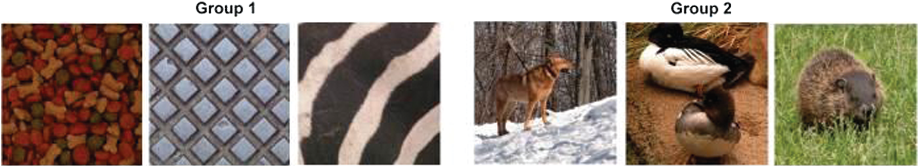
Figure 1: Images for testing: group 1 contain some patterns and those in group 2 are not

In the first test, the convergence performances of the proposed algorithms are verified. The images of dimensions 256×256×3 are used for the proposed methods. The patterns used in this test are {K1}=[8,8,1], {K2}=[16,16,1],{K3}=[32,32,1], {K4}=[64,64,1], and the observation rate is set to be 0.2. Note that in order to achieve a good performance, the patterns are suggested to be set as square as possible. By writing ‘JKTP-i,’ ‘IKTP-i,’ ‘JKTP-econ-i’ and ‘IKTP-econ-i,’ i=1,2,3,4, we mean that the proposed approach will use i patterns out if all 4 patterns for data recovery, and the patterns used are randomly selected in each Monte Carlo trial. The PSNR results of the two groups images data under numbers of iteration in Figs. 2 and 3, respectively. It is shown that the JKTP and JKTP-econ algorithms can converge within 15 iterations and the IKTP and IKTP-econ approaches will converge within 25 iterations when the n umber of patterns is larger than 3. In the remainder image and video experiments, the maximum numbers of iteration are set to be 20 and 30 for these methods, respectively, and we will use at least 3 patterns for proposed algorithms.

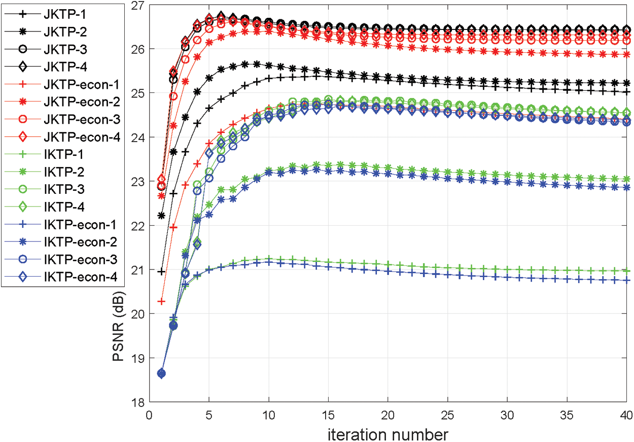
Figure 2: PSNR vs. numbers of iterations with 20% observed entries for group 1 images

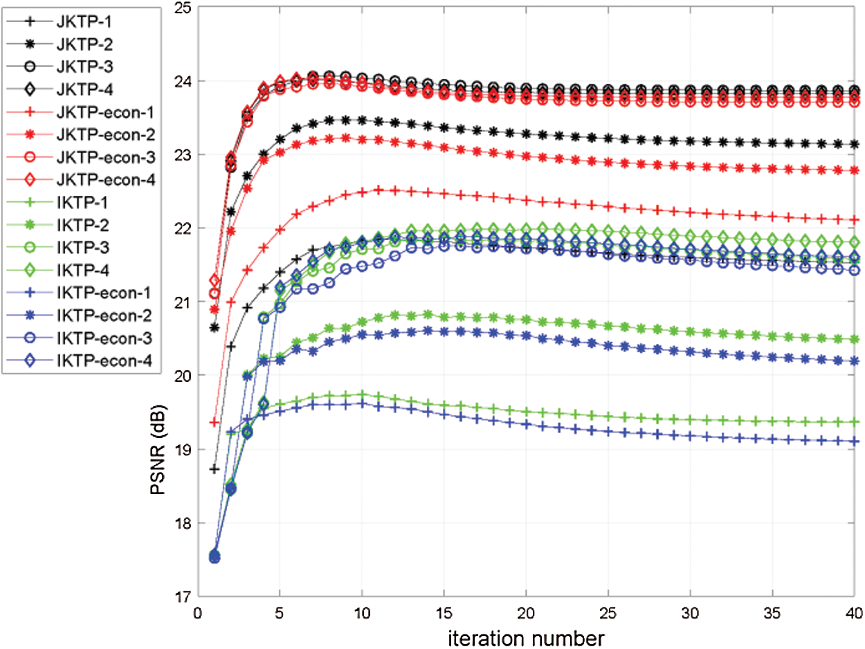
Figure 3: PSNR vs. numbers of iterations with 20% observed entries for group 2 images

In the second test, the completion performances of the proposed approaches under different number of patterns and the state-of-the-art methods for image recovery under 10% observation rate are tested. The four patterns are the same as those in the first test. The average PSNR and SSIM results as well as the computational time in seconds of different methods on the first image, namely, the ‘Group 1: Beans’ under the resolution of 256×256×3 are shown in Tab. 3. Similar performance can be observed for other images in Fig. 1, and thus their recovery results are not shown here. It is shown that when more pattern used, better performance the proposed approached can achieve. Tucker and R1MP methods as well as the KTD approach with i=1,2,3,4 patterns are also included for comparison. It is shown that the JKTP and JKTP-econ methods give inferior results. For i≥2, all the proposed algorithms can give better performance than the Tucker and R1MP approaches. Furthermore, the computational complexity of the proposed methods are much smaller than KTD, making them more attractive in dealing image data.

Table 3: Image recovery performance of different algorithms

In the third test, the performance under different percentage of observation percentages, ranging from 2% to 10 %, is evaluated. The images with resolution 1024×1024×3 are used. We test the proposed methods with 4 patterns {K1}=[16,16,1], {K2}=[32,32,1], {K3}=[64,64,1] and {K4}=[16,16,1]. The other parameters for the proposed approaches are the same as those in the previous test. The PSNR and SSIM results of the two groups images are shown in Figs. 4 and 5, respectively. Generally speaking, the proposed methods can give 3 to 7dB gain over the other algorithms in all cases. The average computational time of the JKTP, JKTP-econ, IKTP, IKTP-econ, KTD, R1MP and Tucker methods are 54.41, 30.54, 14.75, 9.51, 1.57×103, 17.54 and 77.13 s. It is shown that the proposed methods run slightly slower than the R1MP methodology because the R1MP is matrix based rank-1 pursuit method while the proposed methods are tensor based ones. Comparing to the other methods, the computational complexity of proposed algorithms are much smaller, indicating the efficiency of the proposed approaches especially when the dimensions of the data to be recovered is large.

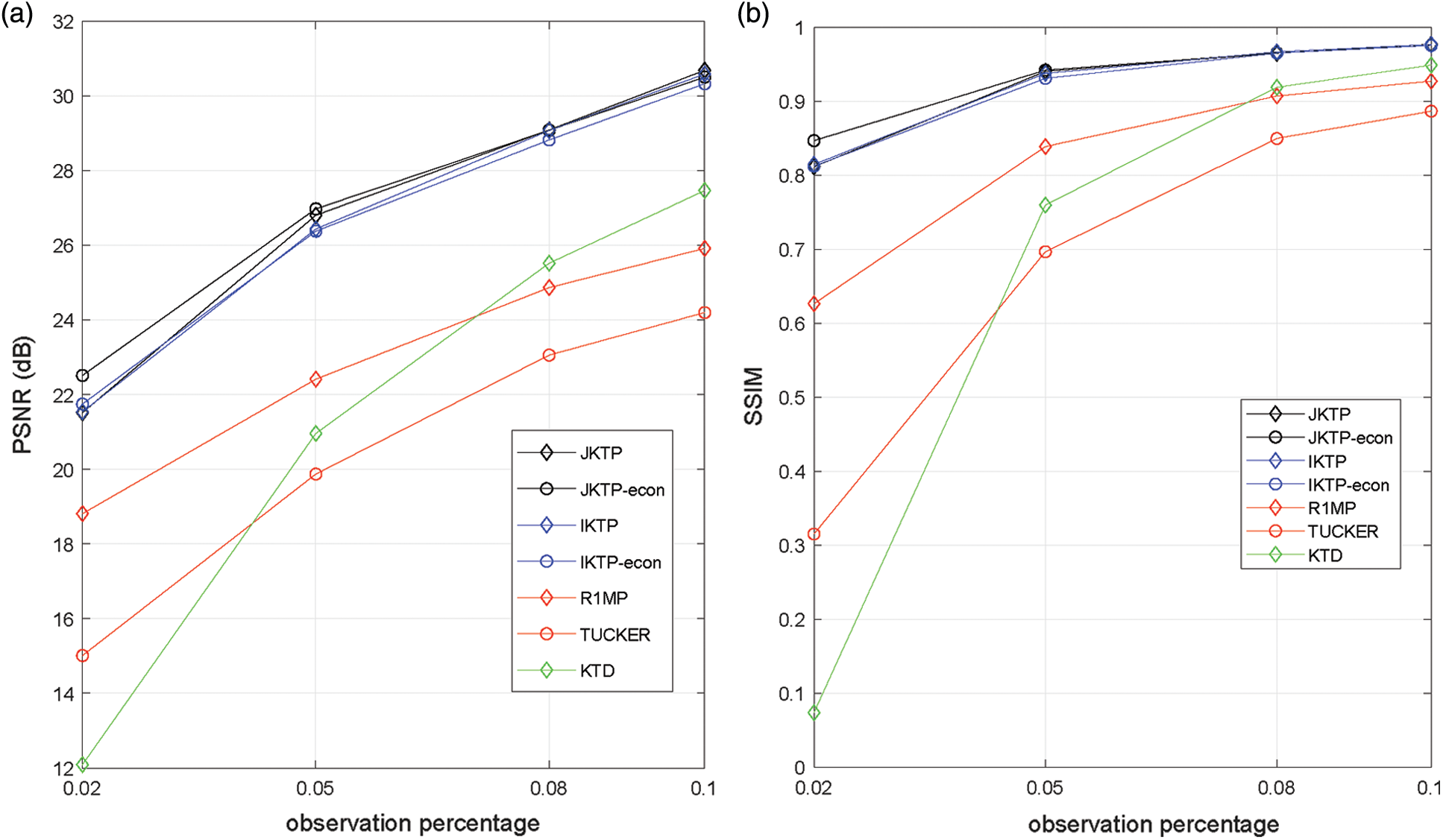
Figure 4: Average PSNR and SSIM vs. observation percentage of group 1 images (a) PSNR (b) SSIM

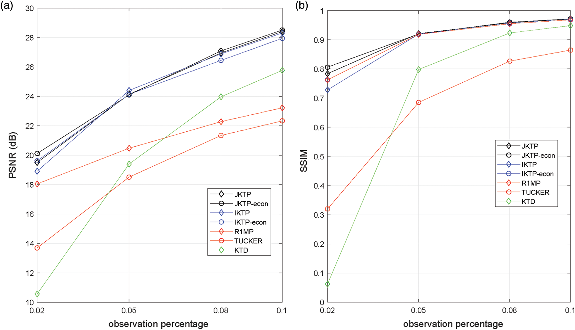
Figure 5: Average PSNR and SSIM vs. observation percentage of group 2 images (a) PSNR (b) SSIM

4.2 Video Inpainting

In this part, we test the algorithms JKTP, JKTP-econ, IKTP, IKTP-econ, Tucker [15], R1MP [19] and R1TP [21] under ‘Gun Shooting’ video [25,26] completion from randomly sampled entries, and the first and last frames of the video are shown in Fig. 6. Note that the KTD approach is not include for comparison because of its high computational complexity. The video is of dimensions 200×520×3×80.

Figure 6: video data for testing

And the situations of different number of frames ranging from 10 to 80 are tested. The observation rate is set to 0.03, and for all the methods, a maximum number of 50 iterations is used. The patterns for the proposed methods are {K1}=[20,52,3,5], {K2}=[40,104,3,5], {K3}=[50,130,3,5] and {K4}=[20,52,1,5], {K5}=[40,104,1,5], {K6}=[50,130,1,5]. The PSNR and SSIM results are shown in Fig. 7 and the computational complexity results are shown in Fig. 8. Note that for the proposed methods, ‘ −3’ means that only the first 3 patterns are used, while ‘ −6’ means that all 6 patterns are employed in data recovery. Generally speaking, the proposed methods give the best PSNR performance when the number of frames used is higher than 20. It is worth noting that although the proposed methods with 3 patterns perform worse than R1TP method when the number of frames used is less than 20, when more frames are used, the recovery performance of the proposed approaches increase rapidly, and far outperform the other methods.

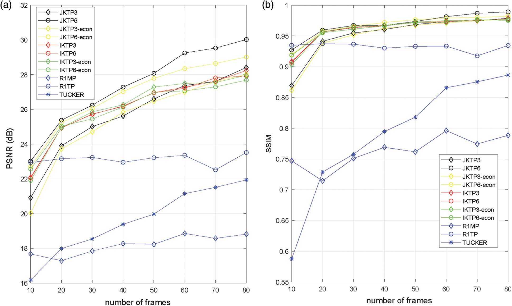
Figure 7: PSNR and SSIM results vs. number of frames (a) PSNR (b) SSIM

Figure 8: Computational complexity vs. number of frames

4.3 High Resolution SAR Imaging

In the end, we evaluate the algorithms with under-sampled high resolution SAR imaging data [27,28]. We employ the model shown in Fig. 9 to conduct our experiments as follows. First, scan the test scene to generate the data X by using the SAR system, and the scanning parameters follow those in [27]. Note that the true image I can be computed from the data X by the FFT process. Furthermore, the data X can be sampled randomly under an observation rate to obtain MΩ. Finally, the tensor recovery methods can be applied for the recovery of the original data as X^, and the recovered image can be computed as I^. The mean square error (MSE) between X and X^ is used to evaluate the performance of the proposed four methods, R1MP [27], Tucker [18] and KTD [22] methods. The tested high resolution SAR imaging scene with the size 6200×12000 is shown in Fig. 10a.

Figure 9: Model of SAR image recovery

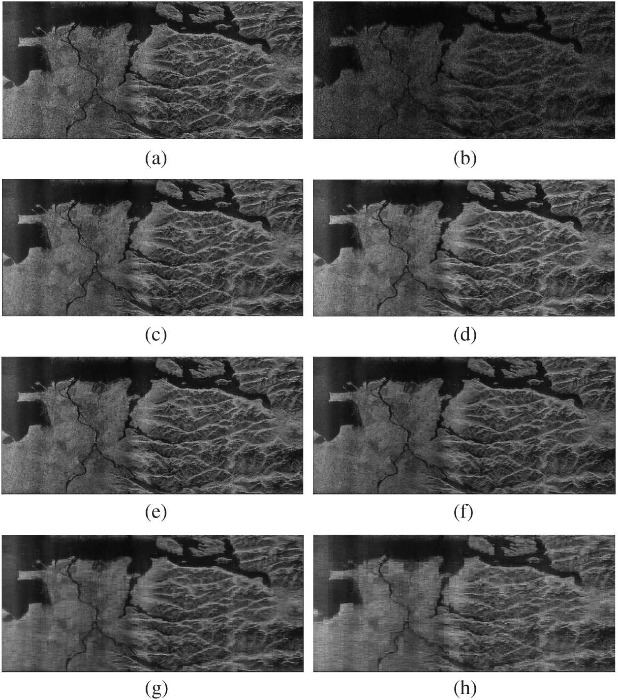
Figure 10: The original, sampled and recovered SAR images (a) Original (b) Sampled (c) JKTP (d) JKTP-econ (e) IKTP (f) IKTP-econ (g) R1MP (h) Tucker

Considering that the size 6200×12000 of the SAR imaging data is too large to be computed effectively by one computer, we will not complete the whole SAR data in one tune. We complete small subdata whose data dimensions are 620×50, 620×200 and 620×400 in one time and repeat the process for 2400, 600 and 300 times, respectively, for the whole image. The patterns for the proposed methods with different completed data size are {K150}=[124,5], {K250}=[62,10], {K350}=[155,5], {K450}=[155,2], {K550}=[124,10], {K650}=[62,5], {K750}=[124,2], {K850}=[620,1], {K1200}=[60,20], {K2200}=[62,25], {K3200}=[124,10], {K4200}=[155,10], {K5200}=[155,8], {K6200}=[124,8], {K7200}=[124,20], {K8200}=[155,20], {K1400}=[124,20], {K2400}=[124,16], {K3400}=[155,16], {K4400}=[62,40], {K5400}=[124,25], {K6400}=[155,20], {K7400}=[155,10], {K8400}=[62,20]. The situations of different observation percentages ranging from 10% to 30% are tested and a maximum number of 40 iterations is used. The SAR imaging scene sampled under the observation percentage 10% is shown in Fig. 10b, and the SAR imaging scenes with the size of 620×200 recovered by all the algorithms under 10% observation rate are shown in Figs. 10c–10f. The completion results of the four methods including MSE performances and CUP times are listed in Tab. 4. Generally speaking, the proposed methods can give the best performance with moderate computational complexity among all the algorithms.

Table 4: Completion results with different step-sizes of completion under 10% to 30% observed entries

5  Conclusion

In this paper, the novel tensor completion algorithms combining the ideas of tensor Kronecker Decomposition and rank-1 tensor pursuit, named IKTP and JKTP, are proposed and applied to color image, video and SAR image inpainting. A novel weight update algorithm, to reduce the time and storage complexity, is also derived. Experimental results show that the proposed methods outperform the state-of-the-art algorithms in terms of PSNR, SSIM and MSE. For the tensor based algorithms, the results also show the advantage of the proposed methods in terms of computational complexity.

Funding Statement: The work described in this paper was supported in part by the Foundation of Shenzhen under Grant JCYJ20190808122005605, and in part by National Science Fund for Distinguished Young Scholars under grant 61925108, and in part by the National Natural Science Foundation of China (NSFC) under Grant U1713217 and U1913203.

Conflicts of Interest: The authors declare that they have no conflicts of interest to report regarding the present study.

References

 1.  L. Gongshen, M. Kui, D. Jiachen, J. P. Nees, G. Hongyi et al., “An entity-association-based matrix factorization recommendation algorithm,” Computers, Materials & Continua, vol. 58, no. 1, pp. 101–120, 2019. [Google Scholar]

 2.  H. Bai, X. Li, L. He, L. Jin, C. Wang et al., “Recommendation algorithm based on probabilistic matrix factorization with adaboost,” Computers, Materials & Continua, vol. 65, no. 2, pp. 1591–1603, 2020. [Google Scholar]

 3.  N. Li and B. Li, “Tensor completion for on-board compression of hyper-spectral images,” in 17th IEEE Int. Conf. on Image Processing, Hong Kong, China, pp. 517–520, 2010. [Google Scholar]

 4.  J. Bengua, H. Phien, H. Tuan and M. Do, “Efficient tensor completion for color image and video recovery: Low-Rank tensor train,” IEEE Transaction on Image Processing, vol. 26, no. 5, pp. 2466–2479, 2017. [Google Scholar]

 5.  S. Gandy, B. Recht and I. Yamada, “Tensor completion and low-n-rank tensor recovery via convex optimization,” Inverse Problem, vol. 27, no. 2, pp. 25–43, 2011. [Google Scholar]

 6.  H. Yang, J. Yin and Y. Yang, “Robust image hashing scheme based on low-rank decomposition and path integral LBP,” IEEE Access, vol. 7, pp. 51656–51664, 2019. [Google Scholar]

 7.  R. Cheng and D. Lin, “Based on compressed sensing of orthogonal matching pursuit algorithm image recovery,” Journal of Internet of Things, vol. 2, no. 1, pp. 37–45, 2020. [Google Scholar]

 8.  L. Vandenberghe and S. Boyd, “Semidefinite programming,” SIAM Review, vol. 38, no. 1, pp. 49–95, 1996. [Google Scholar]

 9.  M. Fazel, H. Hindi and S. P. Boyd, “A rank minimization heuristic with application to minimum order system approximation,” in Proc. of the American Control Conf., Arlington, VA, USA, pp. 4734–4739, 2001. [Google Scholar]

10. M. Fazel, “Matrix rank minimization with applications,” Stanford University: Department of Electrical Engineering, Ph.D. thesis, 2002. [Google Scholar]

11. J. F. Cai, E. J. Candes and Z. Shen, “A singular value thresholding algorithm for matrix completion,” SIAM Journal on Optimization, vol. 20, no. 4, pp. 1956–1983, 2010. [Google Scholar]

12. P. Jain, R. Meka and I. S. Dhillon, “Guaranteed rank minimization via singular value projection,” Advanced in Neural Information Processing, vol. 20, no. 4, pp. 1956–1982, 2008. [Google Scholar]

13. T. G. Kolda and B. W. Bakder, “Tensor decompositions and applications,” SIAM Review, vol. 51, no. 3, pp. 455–500, 2009. [Google Scholar]

14. V. D. Silva and L. H. Lim, “Tensor rank and the ill-posedness of the best low-rank approximation problem,” SIAM Journal on Matrix Analysis Applications, vol. 30, no. 32, pp. 1084–1127, 2008. [Google Scholar]

15. W. Sun and H. C. So, “Accurate and computationally efficient tensor-based subspace approach for multi-dimensional harmonic retrieval,” IEEE Transactions on Signal Processing, vol. 60, no. 10, pp. 5077–5088, 2012. [Google Scholar]

16. T. Thieu, H. Yang, T. Vu and S. Kim, “Recovering incompelte data using tucker model for tensor with low-n-rank,” International Journal of Bioscience, Biochemistry and Bioinformatics, vol. 12, no. 3, pp. 34–40, 2016. [Google Scholar]

17. M. Kilmer and C. Martin, “Factorization strategies for third-order tensors,” Linear Algebra and Its Application, vol. 465, no. 3, pp. 641–658, 2011. [Google Scholar]

18. Z. Zhang and S. Aeron, “Exact tensor completion using t-SVD,” IEEE Transaction on Signal Processing, vol. 65, no. 6, pp. 1511–1526, 2017. [Google Scholar]

19. A. H. Phan, A. Cichocki, P. Tichavsky, D. P. Mandic and K. Matsuoka, “On revealing replicating structures in multiway data: A novel tensor decomposition approach,” in Proc. of Latent Variable Analysis and Signal Separationinternational Conf., Tel Aviv, Israel, pp. 297–305, 2012. [Google Scholar]

20. M. Wang, K. D. Duc, J. Fischer, G. Luta and A. Brockmeier, “Operator norm inequalities between tensor unfoldings on the partition lattice,” Linear Algebra and Its Application, vol. 520, no. 1, pp. 44–66, 2017. [Google Scholar]

21. W. Sun, L. Huang, H. C. So and J. J. Wan, “Orthogonal tubal rank-1 tensor pursuit for tensor completion,” Signal Processing, vol. 157, no. 2, pp. 213–224, 2019. [Google Scholar]

22. Z. Wang, M. J. Lai, L. Lu, W. Fan, H. Davulcu et al., “Orthogonal rank one matrix pursuit for low rank matrix completion,” SIAM Journal on Scientifific Computing, vol. 37, no. 1, pp. A488–A514, 2014. [Google Scholar]

23. M. Jaggi and M. Sulovsk, “A simple algorithm for nuclear norm regularized problems,” in Int. Conf. on Machine Learning, Haifa, Isreal, 2010. [Google Scholar]

24. M. Dudik, Z. Harchaoui and J. Malick, “Lifted coordinate descent for learning with trace-norm regularization,” in AISTATS, La Palma, Canary Islands, Spain, 2012. [Google Scholar]

25. “Pistol shot recorded at 73,000 frames per second,” Published by Discovery, 2015. [Online]. Available: https://youtu.be/7y9apnbI6GA. [Google Scholar]

26. W. Wang, V. Aggarwal and S. Aeron, “Efficient low rank tensor ring completion,” in IEEE Int. Conf. on Computer Vision, Venice, Italy, pp. 5698–5706, 2017. [Google Scholar]

27. D. Yang, G. S. Liao, S. Q. Zhu, X. Yang and X. P. Zhang, “SAR imaging with undersampled data via matrix completion,” IEEE Geoscience and Remote Sensing Letters, vol. 11, pp. 9, 2014. [Google Scholar]

28. S. Zhang, G. Dong and G. Kuang, “Matrix completion for downward-looking 3-D SAR imaging with a random sparse linear array,” IEEE Transactions on Geoscience and Remote Sensing, vol. 56, no. 4, pp. 1994–2006, 2018. [Google Scholar]

This work is licensed under a Creative Commons Attribution 4.0 International License, which permits unrestricted use, distribution, and reproduction in any medium, provided the original work is properly cited.