Computers, Materials & Continua DOI:10.32604/cmc.2021.016825
Article

An Optimal Classification Model for Rice Plant Disease Detection

R. Sowmyalakshmi1, T. Jayasankar1,*, V. Ayyem Pillai2, Kamalraj Subramaniyan3, Irina V. Pustokhina4, Denis A. Pustokhin5 and K. Shankar6

1Department of Electronics and Communication Engineering, University College of Engineering, BIT Campus, Anna University, Tiruchirappalli, 620024, India
2Department of Electronics and Communication Engineering, Gokaraju Rangaraju Institute of Engineering and Technology, Hyderabad, 500090, India
3Department of Electronics and Communication Engineering, Karpagam Academy of Higher Education, Coimbatore, 641021, India
4Department of Entrepreneurship and Logistics, Plekhanov Russian University of Economics, Moscow, 117997, Russia
5Department of Logistics, State University of Management, Moscow, 109542, Russia
6Department of Computer Applications, Alagappa University, Karaikudi, 630001, India
*Corresponding Author: T. Jayasankar. Email: jayasankar27681@gmail.com
Received: 13 January 2021; Accepted: 17 February 2021

Abstract: Internet of Things (IoT) paves a new direction in the domain of smart farming and precision agriculture. Smart farming is an upgraded version of agriculture which is aimed at improving the cultivation practices and yield to a certain extent. In smart farming, IoT devices are linked among one another with new technologies to improve the agricultural practices. Smart farming makes use of IoT devices and contributes in effective decision making. Rice is the major food source in most of the countries. So, it becomes inevitable to detect rice plant diseases during early stages with the help of automated tools and IoT devices. The development and application of Deep Learning (DL) models in agriculture offers a way for early detection of rice diseases and increase the yield and profit. This study presents a new Convolutional Neural Network-based inception with ResNset v2 model and Optimal Weighted Extreme Learning Machine (CNNIR-OWELM)-based rice plant disease diagnosis and classification model in smart farming environment. The proposed CNNIR-OWELM method involves a set of IoT devices which capture the images of rice plants and transmit it to cloud server via internet. The CNNIR-OWELM method uses histogram segmentation technique to determine the affected regions in rice plant image. In addition, a DL-based inception with ResNet v2 model is engaged to extract the features. Besides, in OWELM, the Weighted Extreme Learning Machine (WELM), optimized by Flower Pollination Algorithm (FPA), is employed for classification purpose. The FPA is incorporated into WELM to determine the optimal parameters such as regularization coefficient C and kernel γ. The outcome of the presented model was validated against a benchmark image dataset and the results were compared with one another. The simulation results inferred that the presented model effectively diagnosed the disease with high sensitivity of 0.905, specificity of 0.961, and accuracy of 0.942.

Keywords: Agriculture; internet of things; smart farming; deep learning; rice plant diseases

1  Introduction

Agriculture is the most important source of income for human beings across the globe [1]. The farmers practice agriculture and cultivate crops based on the type of soil and environmental conditions. Unfortunately, farmers experience a lot of challenges such as natural calamities, limited water supply, crop infection, and so on. The application of advanced scientific technology intends to mitigate such issues. By curing plant disease at early stages, one can maximize the yield from plants for which no professional is required. Particularly, plant disease prediction in agriculture is one of the important areas to be investigated in detail [2]. There is a growing need for prediction and classification of crop diseases these days, thanks to increasing awareness about the importance of agriculture and food production.

Indian population is undergoing phenomenal growth due to which cultivation and agricultural practices should also be improved robustly. Being a staple crop, Rice is the most sought-after food crop in India across the nation [3]. However, rice is such a crop that is most likely to get affected by plant diseases, which in turn affects the cultivation and net profit. In order to recover from such problems and to enhance crop cultivation, plant diseases should be predicted and prevented at early stages itself [4]. Sustainable farming can be accomplished by regular disease verification and one should adopt routine plant health observation as a policy. Various investigations have been conducted in plant disease detection so far, which refer that the diseases could be transparent so that the observation process becomes simple and elegant. At most of the times, manual prediction of crop infection goes inaccurate and irregular which complicates the practice. Human intervention is time-consuming and requires better experience in finding the actual name of the disease. Thus, researchers introduced plant disease prediction with the help of IoT, AI and image processing models [5].

In order to overcome the issues discussed above, various hybrid methods have been proposed that generated supreme results. Internet of Things (IoT) is defined as a consortium of sensing devices, communication components, and users. IoT has the capability to generate a superior opportunity through which energetic industrial networks as well as real-world domains can be developed through the deployment of wireless sensors. It becomes possible to combine and introduce the observation mechanism in data gathering with the help of IoT and embedded mechanism. The application of IoT is the prominent step in this network. This is because it possesses an inference module to predict plant diseases and categorize it under nutrient insufficiency by applying wireless communication system. This system is considered to be an optimal path in the mitigation of issues involved in prediction and grouping of plant diseases. Next, the dataset gathered from farming is leveraged to create agriculture hazard alerting technology and corresponding Decision Support System (DSS). The selection of best features is highly significant as IoT information is produced in a fast manner. The availability of massive and dissimilar data mitigates the generalization function. However, this problem can be overcome with the application of Machine Learning (ML) technique which is enhanced with classification accuracy by reducing the count of parameters.

Image processing technique has few steps to be followed in disease detection such as image acquisition, preprocessing, segmentation, feature extraction and classification [6]. These operations are performed upon physical examination of the infected crops [7]. Usually, a plant’s disease can be predicted by observing its major components such as leaves and stems. The signs of plant diseases vary from one another. Further, plant infection varies in color, size, and texture whereas each disease has unique parameters. Few diseases induce yellow coloration while few turn the green leaves into brown [8,9]. Additionally, diseases turn the shape of the plant leaves without changing its color and its vice versa too. Once the infected portion of the plants are segmented, the general portion with disease features should be obtained. Manual prediction of disease through naked eye is time-consuming, inaccurate at times and increases the cost incurred. It is complex to estimate and prone to err while predicting the type of disease [10]. These issues arise due to insufficient knowledge about the plant. In line with this, if rice plant diseases are not predicted or detected at early stages, it affects rice production as experienced in the last few decades [11].

The current research article introduces a novel Convolutional Neural Network-based inception with ResNset v2 model and Optimal Weighted Extreme Learning Machine (CNNIR-OWELM)-based rice plant disease diagnosis and classification model in smart farming environment. The CNNIR-OWELM method utilizes different IoT devices to capture the images of rice plant and send it to cloud server via internet. The CNNIR-OWELM method makes use of histogram segmentation technique to determine the affected regions in the rice plant image. Moreover, Deep Learning (DL)-based inception with ResNet v2 method is applied for feature extraction. Here, OWELM is deployed for classification purposes. Flower Pollination Algorithm (FPA) is also incorporated with WELM to determine the optimal parameters such as regularization coefficient C and kernel γ. The author used a benchmark image dataset to validate the performance of the presented model.

2  Literature Survey

Few research investigations have been conducted earlier regarding the recognition and classification of rice plant infections. Based on Deep Convolutional Neural Network (DCNN), a new rice plant disease prediction method was deployed by Lu at al. [12]. In this research, a dataset with massive images of normal and abnormal paddy stems as well as leaves was applied. Followed by, classification was performed with general rice infections. The study produced results with better accuracy in comparison with traditional ML scheme. The performance result showed the efficiency and possibility of the presented method. For estimating the Region Of Interest (ROI), a segmentation model, relied on neutrosophic logic that was attained from fuzzy set, was established by Dhingra et al. [13]. Here, three Membership Functions (MFs) were applied for segmentation process. In order to predict whether plant leaf is affected or not, feature subsets were used according to the segregated sites.

Different classification methods are in use for representation whereas Random Forest (RF) model resolves alternate models. In this framework, a dataset with defected and non-defected leaf images is employed. Under the application of IP modules, Nidhis et al. [14] introduced a scheme to predict the disease and its type in paddy leaves. The intensity of the disease can be measured by estimating the infected region. Based on the severity of disease, the pesticides are applied to tackle bacterial blight, brown spot, and rice blast which are assumed to be major diseases that affect paddy crops and its yield. Islam et al. [15] proposed a novel technique for prediction and classification of rice plant disease. Here, based on the proportion of RGB value of the affected portion, the disease is identified using IP technique.

Here, Naïve Bayes (NB) classifier is a simple classification model used for classifying the disease into diverse classes. This classifer analyzed and classified the rice plant infection into three major classes with the help of a single feature. Hence, it is a robust mechanism that consumes the minimum computation time. Under the application of IP schemes, disease prediction is performed automatically in paddy leaves as intended [16]. In this study, hybridized grayscale cooccurrence matrix, Discrete Wavelet Transform (DWT), and Scale Invariant Feature Transform (SIFT) were applied for feature extraction. The features were first extracted and induced to different ML-based classifiers for the purpose of classifying normal and abnormal crops.

Kaya et al. [17] examined the simulation outcomes of four various Transfer Learning (TL) methods for Deep Neural Network (DNN)-based plant classification on four general datasets. This work has illustrated that TL is capable of providing essential advantages for automatic plant prediction and improve the performance of plant disease classifiers. A CNN model was employed in the study conducted earlier [18] to compute weed prediction in soybean crop photographs and categorize the weeds between grass and broadleaf. The image database has been developed with numerous images of soil, soybean, broadleaf as well as grass weed. CNN is applied for DL to gain the maximum simulation outcomes in image recognition.

3  Problem Formulation

In the prediction of rice leaf disease, classical models like human vision-related models are applied. An expert suggestion is required here whereas it is time consuming, costly and possess dense limitations. The correctness of human vision model depend upon the eyesight of the expert. ML-related model is activated to find the classes of diseases, to make proper decisions, and to decide on better remedy. The benefit of using ML models is that it computes consistent tasks compared to experts. Hence, to overcome such limitations of previous technologies, a novel ML-based classifier has to be developed. However, there is a gap exists in both detection and classification due to less development in this ML-based plant leaf disease prediction domain.

4  The Proposed Rice Plant Disease Diagnosis Model

Fig. 1 shows the block diagram of the proposed model for rice plant disease detection. The flowchart depicts the flow of events i.e., the IoT devices primarily capture the images of rice plant from farming region and transmits it to cloud server for processing. The proposed method is executed at the server side by incorporating a set of processes such as preprocessing, segmentation, feature extraction, and finally classification. The input images are preprocessed to improve the contrast level of the image. In addition, histogram-based segmentation approach is introduced to detect the diseased portions in rice crop image. Followed by, the feature vectors of the segmented image are extracted by Inception with ResNet v2 model. Subsequently, the extracted feature vectors are fed into FPA-WELM model for classification of the plant disease.

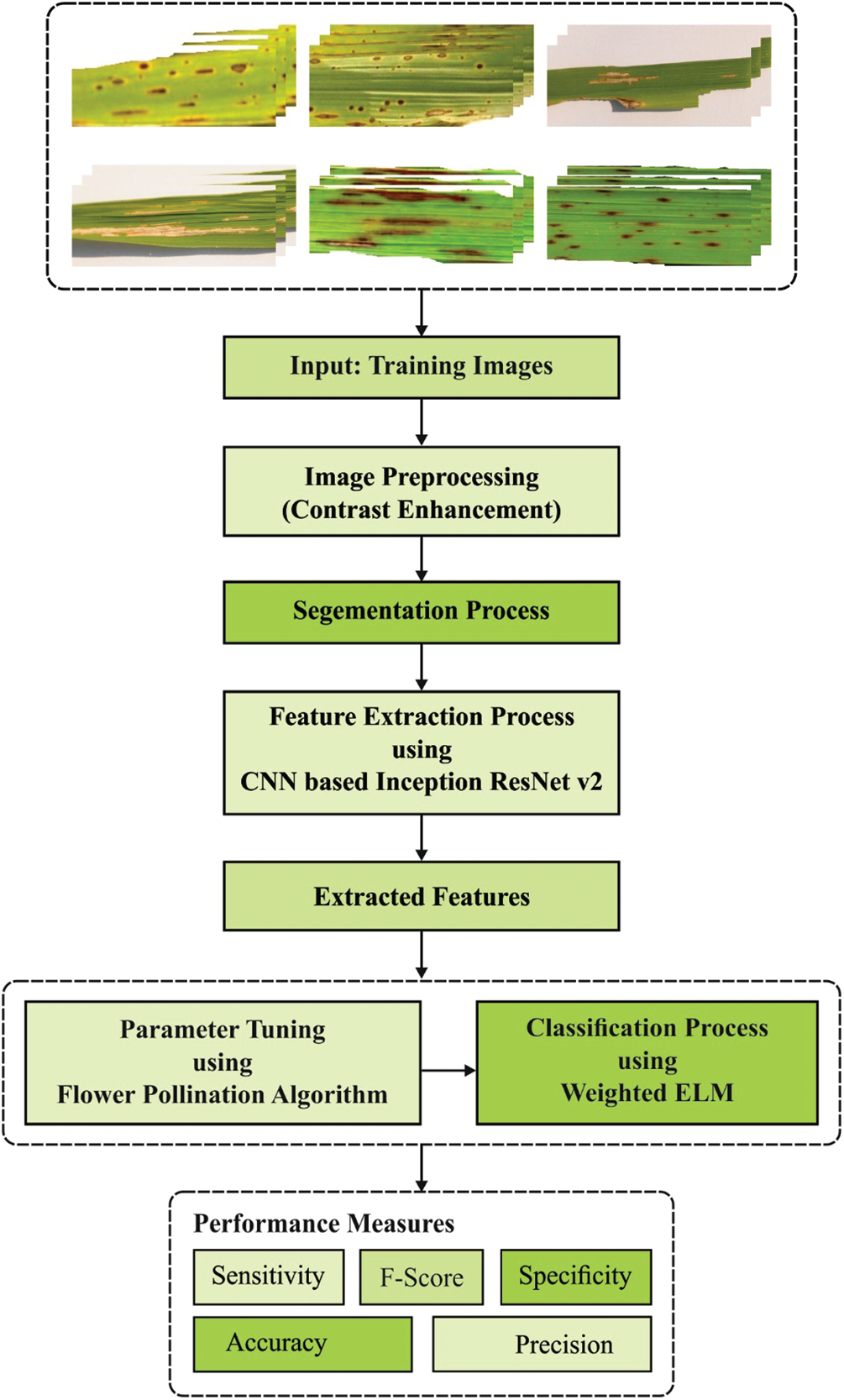
Figure 1: Overall process of the proposed method

4.1 Pre-Processing

In order to accomplish the best classification and segmentation of rice plant images, Contrast Limited Adaptive Histogram Equalization (CLAHE) method is deployed to enhance the density of contrast image. The modified CLAHE is useful in this process to discard noise amplification. Further, various histograms are computed using CLAHE in which the nodes depend upon the standard image region. The histogram gets disseminated to remove the additional amplification whereas the remapping intensity measures are determined through shared histogram. For rice plant images, the newly-developed CLAHE scheme is deployed to enhance the contrast nature of the image. In order to describe the efficacy of CLAHE, few procedures are employed namely entire input production, input pre-processing, processing of background region that intends to develop a mapping to grayscale, and attaining the concluded CLAHE image from random gray level mapping.

4.2 Image Segmentation

Segmentation is defined as the classification of image into a set of non-overlapping parts. Through the identification of optimal threshold values, one can achieve proficient segmentation than the alternate models depending upon the computation of histograms. An image histogram shows reliable frequency for different colors based on its existence such as grayscale level of the input image. Additionally, a digital image can be projected with a value of L colors, while the histogram is assumed as a discrete function as illustrated in Eq. (1),

h(gk)=nkN,K=0,1,…,L-1(1)

where the count of pixels is nk with color gk and it is assumed as a fraction of entire pixels N. So, an exclusive constraint of objects as well as background is pointed out in image histogram, when deep and narrow valleys from the mountains are applied. Hence, the measure for threshold can be selected from the termination of valley.

In general, a global threshold is computed effectively when the peaks in image histogram are of interest and the background is categorized. Furthermore, it is apparent that the current method could not be applied for illuminated images. The valleys of histograms are longer and get expanded with diverse measures of heights. Followed by, a local adaptive threshold finds a threshold for each pixel depending upon the range of intensities, attained from local neighborhood. Next, thresholding is carried out for an image in conjunction with a histogram that lacks original peaks. Moreover, specific methods are employed to split the image into sub images for which the mean value is applied. If a specific feature is involved in an image, then prior to this procedure, the operation of picking a threshold becomes simple whereas the root cause for deciding a threshold is to assure the present task is accomplished. A new technology called P-tile applies data in the form of darker objects when compared to another background. It applies a definite fraction such as percentile (1/p) of complete image ration and for printed sheets. Therefore, a threshold is used for examining the intensity target fraction of image pixels than the previous value. Next, the intensity is found under the application of cumulative histogram:

c(gk)=∑i=0kgi(2)

The measure of threshold T is assigned as sc(T) = 1/p. For a dark background, it is declared as c(T) = 1 −1/p.

4.3 Feature Extraction

The supervised learning model use CNNs with reduced attributes and effective training speed in comparison with deep Artificial Neural Network (ANN) especially with possible advantages like image segmentation, prediction, and classification. A feature map of initial layer is obtained by reducing the input volume after which conv. kernels are applied. Conv. kernel is comprised of 5×5 and the stride is 1. A feature map is derived using the following expression.

nf=ni+2p-fs(3)

where nf means the size of a feature map; ni defines the input size; p indicates the padding score; f shows the kernel size; and s represents the stride values. The basic function of convolution operation is defined as follows.

a1=δ(Wlal-1+bl)(4)

where al means a simulation of lth Conv. layer; wl denotes a Conv kernel of lth Conv layer; al −1 signifies a result of l −1th Conv layer; bl depicts bias of lth Conv layer; and δ stands for the activation function of lth Conv layer. Sub-sampling employs a major object as pooling task. The size of pooling kernel is 2×2 whereas for stride, it is 2. Some of the activation functions are sigmoid, tanh, and ReLU. The parameters attained by Conv layer are forwarded to FC layer; thus, the image classification is performed. Followed by, CNN is composed of different objects like convolution, activation, pooling, FC, and softmax layers. Fig. 2 shows the structure of CNN model.

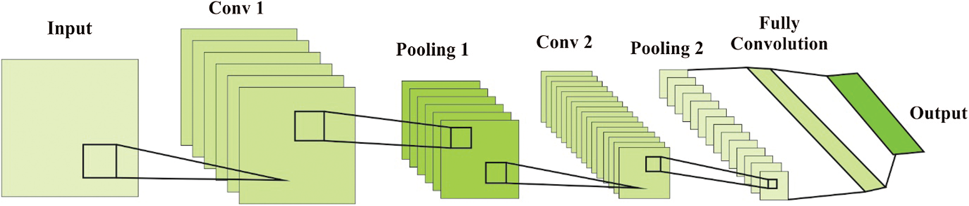
Figure 2: Overview of CNN

Conv. layer contains filters which have to be convolved across the width and height of input data. Besides, the simulation of a Conv. layer is attained with the application of dot product between filter weight content and exclusive location of input image. It is considered that 2D activation map offers filter responses in spatial location. The excess variables are number of filters, filter weight, size, stride, padding, and so on. These variables are used in examining the size of outcome. Typically, pooling layers concentrate on removing the overfitting problems whereas non-linear down-sampling is applied on activation maps that decrease both dimension as well as complexity. Consequently, the computation speed gets improved. The attributes applied are filter size and stride, where padding is not essential in pooling. Furthermore, pooling is applied in input channels effectively. Likewise, both output and input channels are similar. It is classified into two classes namely, max pooling and average pooling.

•    Max pooling: The working principle of this layer is similar to Conv. layer. However, it primarily varies on two aspects i.e., capturing a dot product from input and filter and maximum neighboring value from input image

•    Average pooling: The values are processed by exclusive position from input image

The Fully Connected (FC) layer is also termed as hidden layer and is used for unwanted NN. Next, the input array is changed as 1D vector with the help of a flattening layer. Here, a node in input is connected to all nodes present in the output.

Softmax layer is applied in the layer consequent to CNN, which implies a categorical distribution between labels and it offers the feasibilities of an input that belongs to a class.

The base model for inceptions is applied in the training of diverse portions as the monotonous block is categorized as subnetworks and is generally utilized in the activation of comprehensive process in memory. However, inception technique is referred to as a simple technique that shows the probability of changing the number of filters accomplished from remarkable layers without influencing the heartiness of complete trained network. To improve the training efficiency, a layer size should be changed into better value so that an appropriate trade-off can be attained from diverse sub-networks. Unlike earlier, tensor flow advanced inception methods are deployed without repeated partitioning. Moreover, inception-v4 is applied to eliminate irregular process, which has developed similar mechanism for inception blocks in each grid size.

Each inception block is used by a filter expansion layer that guides in enhancing the dimension of filter bank prior to input depth estimation. Hence, it is a significant task to replace the dimensional cutback that results in the inception block. Among different techniques of inception, Inception-ResNet V2 has gradual speed since it is presented with massive count of layers. The excess alignment between residual and non-residual inception is termed as Batch-Normalization (BN) and is applied in the classical layer rather than being used on residual estimation. Therefore, it is assumed as a logical concept at the time of anticipating a large-scale BN. A BN of TensorFlow applies massive amount of memory and to reduce the number of layers, BN is employed under diverse positions. Fig. 3 shows the blocks in inception ResNet V2 layers.

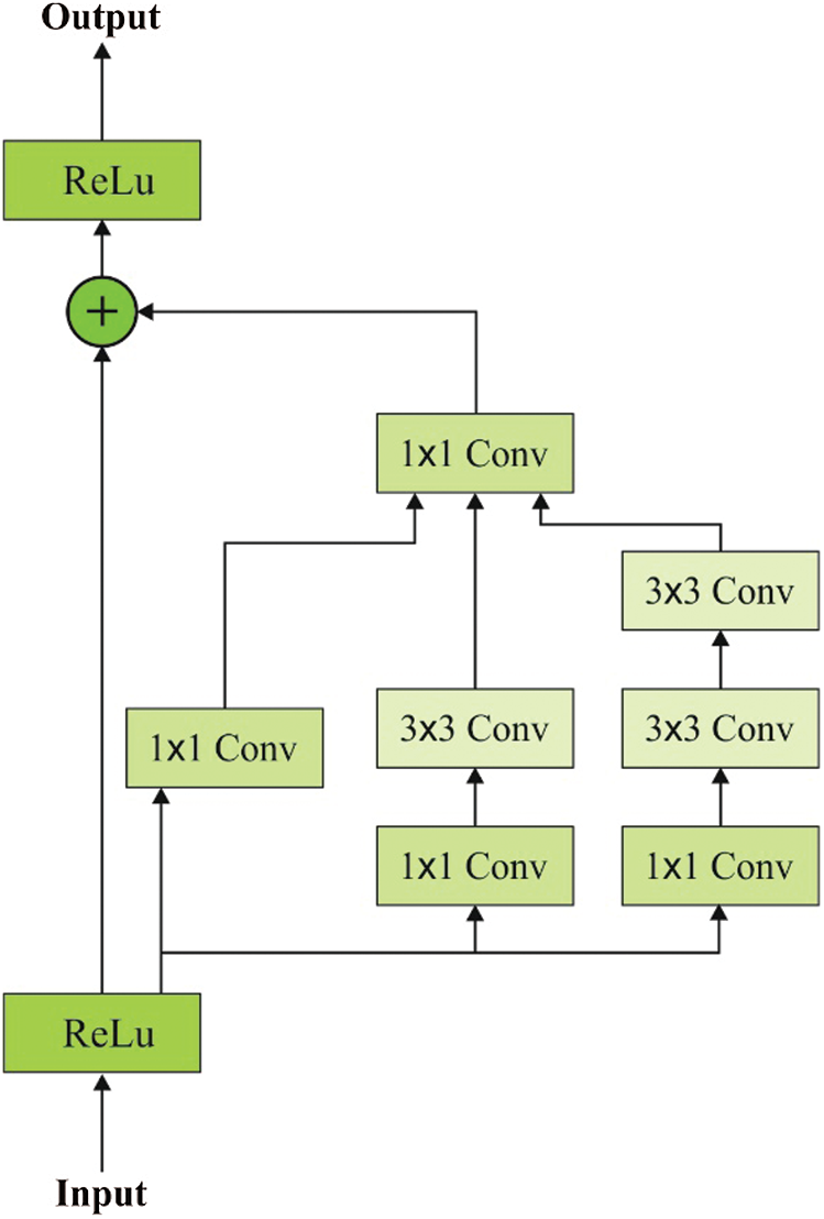
Figure 3: Blocks in inception ResNet V2 layers

Here, it is marked that a filter score can be found. This phenomenon depicts an unreliable system which gets expired during primary phase of training implying that the target layer, prior to initializing a pooling layer, creates the zeros from distinct process. But it is not possible to eliminate the training score. Further, the measures are reduced prior to identification of better learning. Usually, scaling factors exist within the radius of 0.1 to 0.3 and are applied for scaling accumulated layer activations correspondingly.

4.4 OWELM-Based Classification

ELM is utilized in the classification of balanced dataset whereas WELM is utilized in the classification of imbalanced datasets. So, this section briefly establishes WELM. During training, dataset has N different instances, (xi,zi), i=1,2,…,N. A single hidden layer NN with L hidden layer nodes is illustrated as follows:

∑i=1Lβi⋅l(wi⋅xj+bi)=zj,j=1,…,N(5)

where wi is a single hidden layer input weight, l() is an activation function, βi is the resultant weight, and bi is the single hidden layer bias. Eq. (5) is easily written as follows.

Sβ=T(6)

where S is a single hidden layer resultant matrix.

S(wl,…,WL,b1,…,bL,x1,…,xN)=(l(w1⋅χ1+b1)⋯l(wL⋅xN+bL)⋮⋱⋮l(w1⋅xN+b1)⋯l(wL⋅χ1+bL))N×L(7)

Based on Karush-Kuhn-Tucker hypothesis, Lagrangian factor is established to alter the training of ELM into a dual problem. A resultant weight β is computed as follows.

β=ST(1C+SST)-1T(8)

where C is a regularization coefficient. So, the resultant function of an ELM classifier is written as follows.

F(x)=s(x)ST(1c+SST)-1T=[K(x,x1)⋮K(x,xN)](1c+χ)-1T(9)

where χ is a kernel matrix, computed as:

χ=SST=s(xi)s(xj)=K(xi,xj)(10)

It is from (8) it is established that the hidden layer feature map s(x) is independent from the classification result of ELM. Further, the classification result is only transmitted to kernel function K(x,y). Here, K(x,y) takes an inner product type. So, the count of hidden layer nodes has no outcome on the result. Thus, ELM does not require to set the input weights and offsets of the hidden layer. A kernel function of KELM is generally an RBF function:

K(x,y)= exp(-γ∥x-y∥2)(11)

So, KELM classification performance is decided by two parameters such as kernel function parameter γ and penalty parameter C.

To maintain the original benefits of ELM, it is presented that WELM allocates weights to different instances so that imbalanced classification problems can be resolved. Its resultant function is computed as given herewith.

F(x)=[K⋮K]F(x)=[K(x,x1)⋮K(x,xN)]T(1C+Wχ)-1WT (12)

W=diag(wii),i=1,2,…,N (13)

where W is a weight matrix. WELM consists of two weighting systems as given herewith.

wii=1#(zi) (14)

wii={0.618#(zi),ifzi>z¯i1#(zi),otherwise (15)

where #(zi) is the count of samples going to class zi, i=1,…,m. m is the count of classes. z¯i is the average of entire instances in every class. When (14) is implemented in WELM, it is known as WELMI and when implementing (15), it is known as WELM2.

Regularization coefficient C and kernel γ are crucial parameters in this work since it affects the outcome of WELM model. So, these parameters are optimized using FPA. Flower pollination is a complex process in plant creation strategy. Flower and relevant pollen gametes intend to offer a consistent solution for optimization problems. FPA has a lot of benefits. One such benefit is that it offers an elegant flower analogy with minimum weight processing method depending upon single parameter (switch condition, p) in contrast to genetic algorithm (GA), HS, and Particle Swarm Optimization (PSO). Moreover, it provides an equivalent intensification and diversification of solutions under the application of lévy flight and switch condition which are applied for changing both global search and intensive local search.

Flower constancy is defined as the exact solution. For global pollination, a pollinator sends pollen from long distances to higher fitting. Alternatively, local pollination is processed in a tiny region of a flower in shading water. Global pollination is carried out under the feasibility that is termed as ‘switch probability.’ Once the above process is removed, local pollination is deployed. In FPA model, around four rules are present as given herewith.

•    Live pollination and cross-pollination are named as global pollination for which the carriers of pollen pollinator use levy fight algorithm

•    Abiotic and self-pollination are considered to be local pollination

•    Pollinators are nothing but the insects which can develop flower constancy. It is depicted as a production possibility for the flowers.

•    The communication between global and local pollination is balanced using switch possibility.

Therefore, 1st and 3rd rules are illustrated as follows.

xqt+1=xpt+γ×L(λ)×(g*-xpt)(16)

where xpt implies a pollen vector at iteration t; g * denotes the present optimal solution from recently generated outcomes; γ=a refers to scale factor that controls the step size, and L refers to strength of pollination which is related to step size of levy distribution. Levy flight is a collection of random processing, where the length of each jump uses levy probability distribution with indefinite variance. Next, L shows a levy distribution as given herewith.

L~λ×Γ(λ)× sinπλ2π×1S1+λS≫S00(17)

where Γ(λ) represents a remarkable gamma function. For local pollination, 2nd and 3rd rules are depicted as follows

xpt+1=xpt+ε(xqt-xkt)(18)

where xqt and xkt=2. Here, the pollens are collected from various flowers at the same time. In numerical form, xqt and xkt emerge from same species selected from homogeneous population and is implied as a local random walk whereas ε denotes a uniform distribution from [0, 1].

5  Experimental Validation

The performance of the CNNIR-OWELM model was validated using a benchmark rice leaf disease dataset [19]. The dataset comprises of images under three class labels. A total of 40 images under bacterial leaf blight, 37 images under brown spot, and 38 images under leaf smut are present in the data. The details related to the dataset are provided in Tab. 1 and some sample test images are shown in Fig. 4.

Table 1: Dataset description

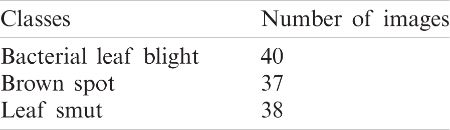
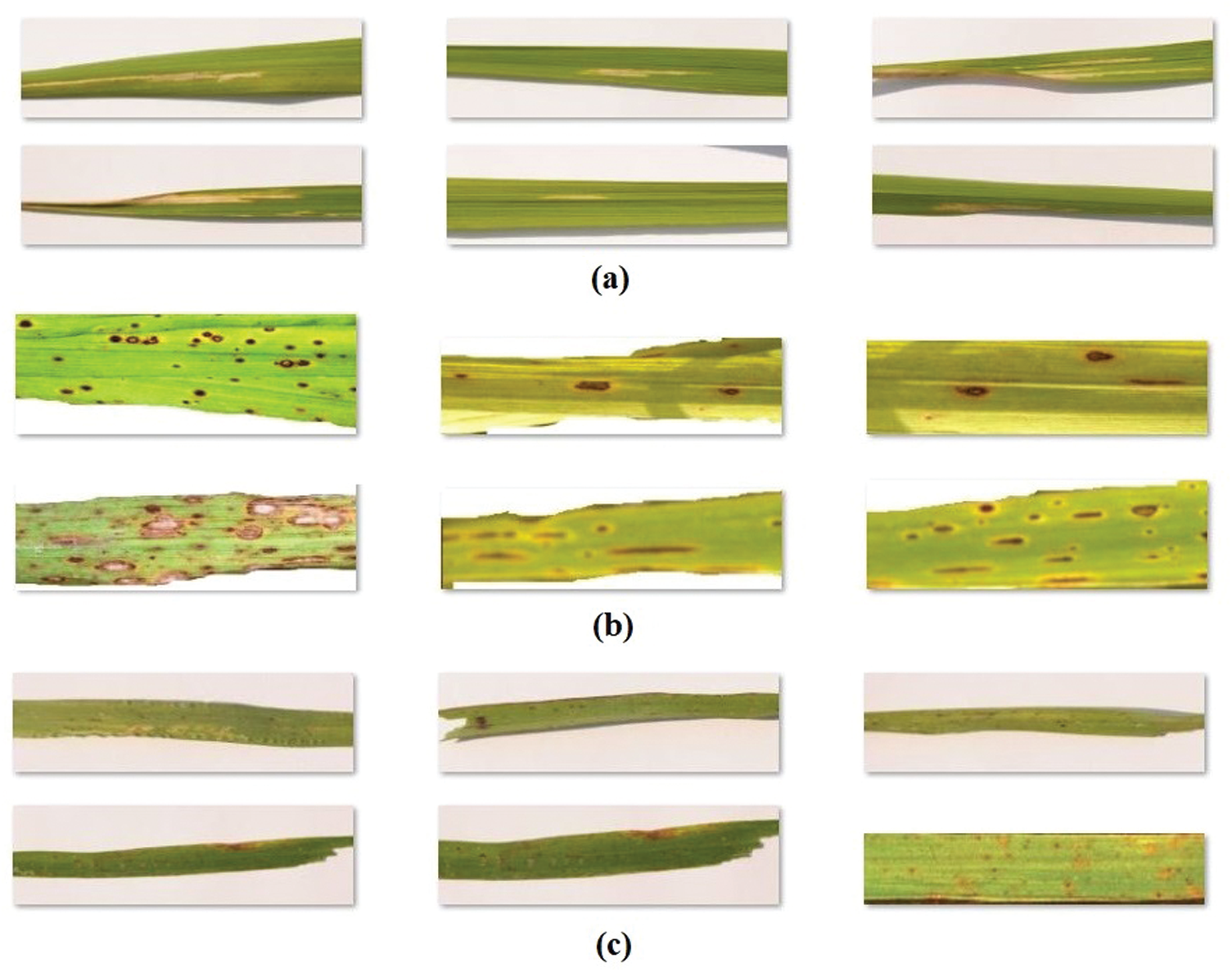
Figure 4: The sample images (a) bacterial leaf blight (b) brown spot (c) leaf smut

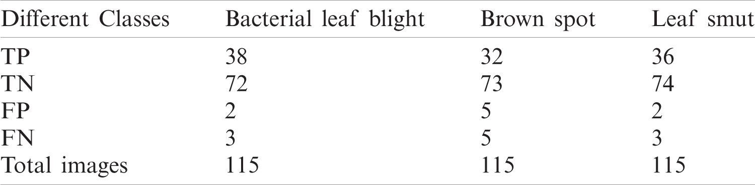
Tab. 2 offers a confusion matrix generated by the proposed CNNIR-OWELM model for the rice plant disease dataset used in this study. The obtained values showcase that the CNNIR-OWELM model effectively classified 38 images under bacterial leaf blight, 32 images under brown spot, and 36 images under leaf smut. These values establish that the CNNIR-OWELM model produce superior results in the identification of rice plant disease.

Table 2: Manipulations from confusion matrix of the proposed CNNIR-OWELM

Tab. 3 and Figs. 5–6 illustrate the identification results of CNNIR-OWELM model upon rice plant disease diagnosis. In terms of classifying bacterial leaf blight, the CNNIR-OWELM model accomplished high sensitivity of 0.927, specificity of 0.973, precision of 0.950, accuracy of 0.957, and F-score of 0.938. Similarly, when classifying Brown Spot, the CNNIR-OWELM method resulted in high sensitivity of 0.865, specificity of 0.936, precision of 0.865, accuracy of 0.913, and F-score of 0.865. Likewise, when classifying leaf smut, the CNNIR-OWELM model produced the maximum sensitivity of 0.923, specificity of 0.974, precision of 0.947, accuracy of 0.957, and F-score of 0.935. Concurrently, the average analysis of CNNIR-OWELM model resulted with a sensitivity of 0.905, specificity of 0.961, precision of 0.921, accuracy of 0.942, and F-score of 0.913.

Table 3: The Performance measures of test images on proposed CNNIR-OWELM

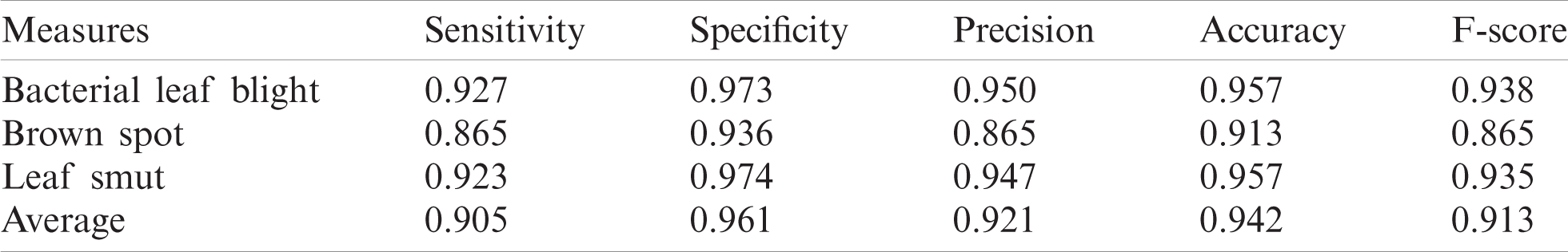
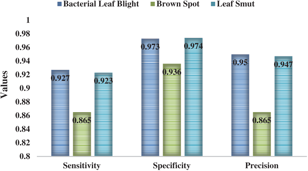
Figure 5: The Result analysis of CNNIR-OWELM model-I

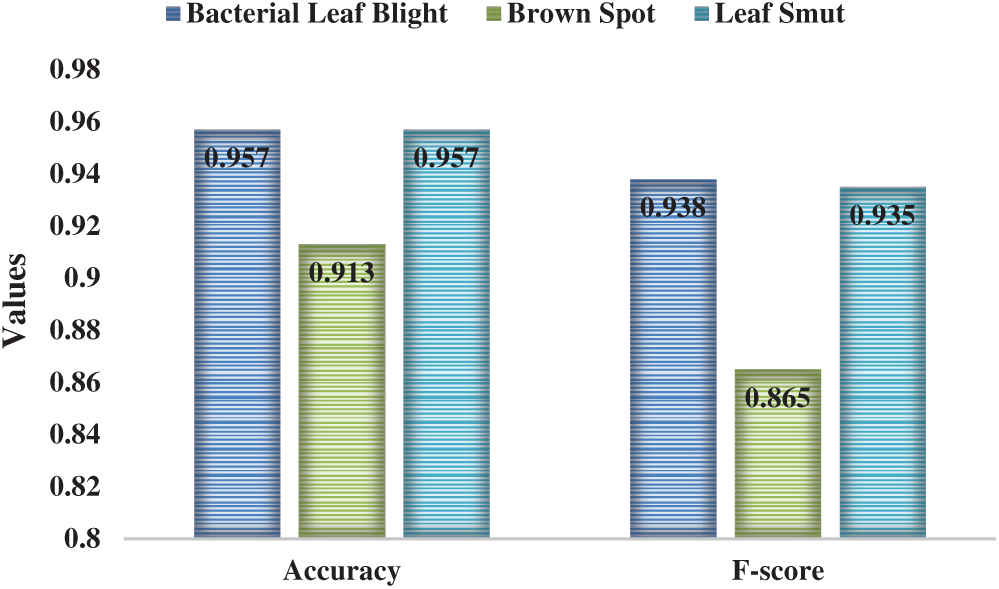
Figure 6: Result of the analysis of CNNIR-OWELM model-II

Tab. 4 provides a detailed comparison on the results of analysis of CNNIR-OWELM model in terms of distinct evaluation parameters. Fig. 7 shows an accuracy analysis of the CNNIR-OWELM model and comparison with existing methods. The figure depicts that the KNN model achieved poor diagnosis of rice plant disease with least accuracy of 0.7. At the same time, the ANN model resulted in slightly higher accuracy of 0.8 whereas even higher accuracy of 0.86 was obtained by DAE model. In line with this, the DNN model attained a moderate accuracy of 0.9 and the SIFT-SVM model reached a certainly high accuracy of 0.911. Simultaneously, the VGG16-CNN model resulted in a manageable performance of 0.929 accuracy. Eventually, the SIFT-KNN model produced superior results than other methods except CNN and CNNIR-OWELM model with an accuracy of 0.933. Though the CNN model obtained a near optimal classification performance with an accuracy of 0.938, the presented model achieved the maximum accuracy of 0.942.

Table 4: Comparison of existing methods with the proposed CNNIR-OWELM method in terms of performance measures

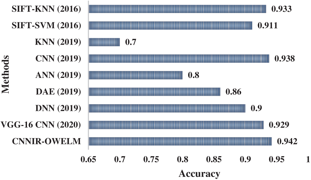
Figure 7: Accuracy analysis of CNNIR-OWELM model

Fig. 8 shows the results achieved from the comparative analysis of CNNIR-OWELM model and other existing models with respect to sensitivity and specificity. The figure demonstrates that the ANN model attained the worst diagnosis for rice plant disease with least sensitivity of 0.633 and specificity of 0.816. Comparatively, the KNN model has resulted in somewhat higher sensitivity of 0.65 and specificity of 0.78. The DAE model achieved even more sensitivity of 0.68 and specificity of 0.872. Likewise, the DNN model attained a moderate sensitivity of 0.735 and specificity of 0.894 and the SIFT-SVM model obtained a certainly higher sensitivity of 0.867 and specificity of 0.832. At the same time, the VGG16-CNN model performed well with a sensitivity of 0.898 and specificity of 0.932. Further, SIFT-KNN model attempted to yield higher outcomes over other earlier methods except CNN and CNNIR-OWELM model with the sensitivity of 0.9 and specificity of 0.864. But, the proposed CNNIR-OWELM model performed extremely well compared to all other models with a near optimal classification performance i.e., sensitivity of 0.905 and specificity of 0.961. The CNN model outperformed all the models with highest sensitivity of 0.94 and specificity of 0.94.

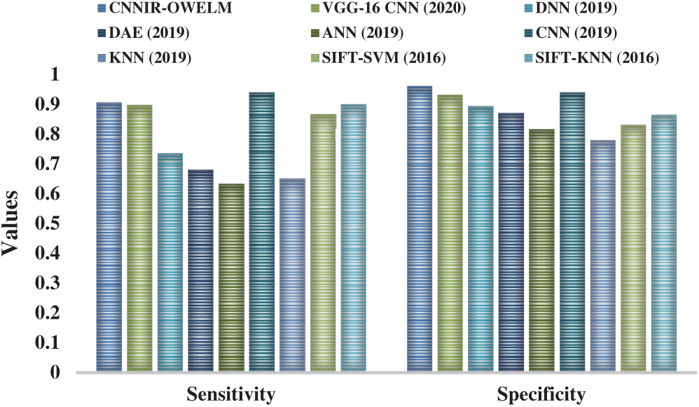
Figure 8: Sensitivity and specificity analysis of CNNIR-OWELM model

Fig. 9 portrays the results accomplished from the comparative analysis of CNNIR-OWELM model with other existing methods with respect to precision and F-score. The figure exhibits that the ANN model attained poor diagnosis for rice plant disease with a minimum precision of 0.609 and F-score of 0.683. In line with this, the DAE model yielded a slightly higher precision of 0.676 and F-score of 0.77 whereas even higher precision of 0.72 and F-score of 0.65 was obtained by KNN model. Among these, the DNN model attained a moderate precision of 0.749 and F-score of 0.815 while the SIFT-SVM model attained a certainly superior precision of 0.867 and F-score of 0.867. At the same time, the VGG16-CNN model resulted in a manageable performance with the precision of 0.902 and F-score of 0.899. Eventually, the SIFT-KNN model attempted to demonstrate superior outcomes over earlier methods except CNN and CNNIR-OWELM model with a precision of 0.906 and F-score of 0.901. But the CNNIR-OWELM model attained a near optimal classification performance with its precision value being 0.921 and F-score value being 0.913. The CNN model outperformed all other models with highest precision of 0.94 and F-score of 0.94.

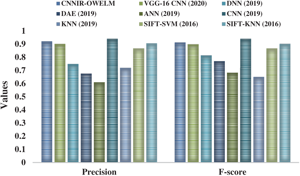
Figure 9: Precision and F-score analysis of CNNIR-OWELM model

6  Conclusion

This research work presented a novel CNNIR-OWELM model for rice plant disease diagnosis in smart farming environment. The proposed method is executed at the server side and incorporates a set of processes such as image collection, preprocessing, segmentation, feature extraction, and finally classification. Primarily, the IoT devices capture the rice plant images from farming region and transmit it to the cloud servers for processing. The input images are preprocessed to improve the contrast level of the image. In addition, the histogram-based segmentation approach is introduced to detect the diseased portions in the image. Followed by, the feature vectors of the segmented image are extracted by Inception with ResNet v2 model. Subsequently, the extracted feature vectors are fed into FPA-WELM model for the classification of rice plant diseases. The experimental outcome of the presented model was validated against a benchmark image dataset and the results were compared with one another. The simulation results infer that the presented model effectively diagnosed the disease with a higher sensitivity of 0.905, specificity of 0.961, and accuracy of 0.942. In the future, the researchers can extend the presented model to diagnose diseases that commonly affect the fruit plants, apart from rice plants.

Funding Statement: The authors received no specific funding for this study.

Conflicts of Interest: The authors declare that they have no conflicts of interest to report regarding the present study.

This work is licensed under a Creative Commons Attribution 4.0 International License, which permits unrestricted use, distribution, and reproduction in any medium, provided the original work is properly cited.