Predicted Oil Recovery Scaling-Law Using Stochastic Gradient Boosting Regression Model

Mohamed El-Amin; Abdulhamit Subasi; Mahmoud Selim; Awad Mousa

doi:10.32604/cmc.2021.017102

1Energy Research Lab., College of Engineering, Effat University, Jeddah, 21478, KSA
2Artificial Intelligence and Cyber Security Research Lab., College of Engineering, Effat University, Jeddah, 21478, KSA
3Department of Mathematics-College of Sciences & Humanities in Al Aflaj, Prince Sattam bin Abdulaziz University, Al-Aflaj, 11912, KSA
4Department of Physics, College of Science & Humanities in Al-Aflaj, Prince Sattam bin Abdulaziz University, Al-Aflaj, 11912, KSA
5Mathematics Department, Faculty of Science, Aswan University, Aswan, 81528, Egypt
*Corresponding Author: Mahmoud M. Selim. Email: m.selim@psau.edu.sa
Received: 21 January 2021; Accepted: 26 February 2021

Abstract: In the process of oil recovery, experiments are usually carried out on core samples to evaluate the recovery of oil, so the numerical data are fitted into a non-dimensional equation called scaling-law. This will be essential for determining the behavior of actual reservoirs. The global non-dimensional time-scale is a parameter for predicting a realistic behavior in the oil field from laboratory data. This non-dimensional universal time parameter depends on a set of primary parameters that inherit the properties of the reservoir fluids and rocks and the injection velocity, which dynamics of the process. One of the practical machine learning (ML) techniques for regression/classification problems is gradient boosting (GB) regression. The GB produces a prediction model as an ensemble of weak prediction models that can be done at each iteration by matching a least-squares base-learner with the current pseudo-residuals. Using a randomization process increases the execution speed and accuracy of GB. Hence in this study, we developed a stochastic regression model of gradient boosting (SGB) to forecast oil recovery. Different non-dimensional time-scales have been used to generate data to be used with machine learning techniques. The SGB method has been found to be the best machine learning technique for predicting the non-dimensional time-scale, which depends on oil/rock properties.

Keywords: Machine learning; stochastic gradient boosting; linear regression; time-scale; oil recovery

The hydrocarbons reservoirs are naturally fractured, so that they consist of two main sections, fractures and matrix blocks (Fig. 1). Fracture permeability is higher than matrix permeability, and the opposite is true for porosity, i.e., the volume of the hydrocarbons in matrix blocks is much bigger than in fractures. In the oil recovery process, water is pumped, and oil is collected into fractures from the matrix blocks and then into wells of production. The imbibition is considered a common mechanism of oil extraction, whereas water pushes oil from the matrix into the adjacent fracture. There are two sorts of imbibition, namely, counter-current imbibition and co-current imbibition. In the co-current imbibition mechanism, water is injected into the matrix from one side to displace oil to the opposite side. On the other hand, in the counter-current imbibition type, water is injected into the matrix and collect oil from the same side. The counter-current is one often mechanism because the matrix block (filled with oil) is surrounded by fractures (filled with water) [1–8]. Usually, experiments are performed on small rock samples to estimate the oil recovery. Therefore, the obtained data are fitted in a non-dimensional equation, called scaling-law. This would help understand real reservoir behavior. This kind of scaling law is a non-dimensional universal variable including primary parameters of rocks and fluids properties. Essentially, when the data are presented in one curve with a few numbers of primary parameters, then we can conclude that the scale is working well.

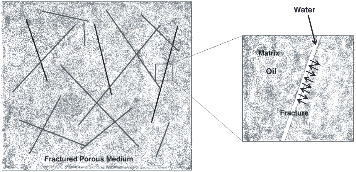
Figure 1: Schematic diagram of the counter-current oil-water imbibition in a fractured rock

In this study, we utilize the SGB machine learning technique to forecast oil recovery estimation and its scaling-law. In general, the ML techniques, including Artificial Neural Networks (ANNs), k-nearest neighbor (k-NN), and Support Vector Machine (SVM), can be utilized to predict oil recovery too. However, most of the well-established machine learning techniques are complex, and their training processes are time-consuming. Rule-based Decision Tree (DT) and tree-based ensembles (TBE) methods such as Random Forest (RF), Extremely Randomized Trees (ERT), and SGB are powerful and robust forecasting algorithms. The ML tools are recently used widely in the oil/gas industry [9] due to their precise assessment of future recovery [9]. Therefore, several oil/gas industry problems can be solved [10–17]. On the other hand, the ANN can be utilized to predict carbonate reservoirs’ permeability based on the well-log data [18–20]. For example, Elkatatny et al. [12] have used the ANN model to predict reservoir well-logs heterogeneous permeability. Although the ANN method estimates the permeability with high precision and minimal log-data, ANN has some problems, such as uncertainty. Also, the support vector machine (SVM) method has been employed to predict reservoir permeability [11]. The SVM scheme has some limitations, including the inability to eliminate uncertainties and the need to confirm the stability/consistency of the scheme. Fortunately, the SGB and RF schemes can sustain the above-mentioned limitations. Those necessities and have not been applied to oil/gas reservoir predictions, such as the current work, which is interested in oil recovery predictions.

The machine learning SGB regression algorithm has been developed to predict oil recovery from oil reservoirs based on laboratory measurements and analytical models. To the best of the author’s knowledge, the machine learning tools have not been used before in oil recovery prediction. The performance of oil recovery prediction is assured for the SGB model. Also, other machine learning techniques, including k-NN, ANN, SVM, and RF, have been used oil recovery besides the SGB model. Another significant coefficient in oil recovery prediction, namely, the universal dimensionless time, has also been predicted along with oil recovery in a generalized scaling-law [8].

In this paper, a novel ensemble prediction scheme is utilized to accomplish oil recovery prediction. The proposed model utilizes the SGB model for oil recovery. The rest of the paper is arranged as follows: In Section 2, scaling laws are discussed. In Section 3, machine learning techniques are explained. Section 4 provides the results and discussions; and finally, conclusions are presented in Section 5.

Aronofsky et al. [21] have introduced an analytical formula of the oil recovery against the dimensionless time, i.e.,

where α=0.05 [-] is a rate coefficient [22], T [-] is the dimensionless time, R [m3] is the recovery, Rim [m3] is the ultimate. Tab. 1 presents the most common analytical time-scales that can be found in the literature.

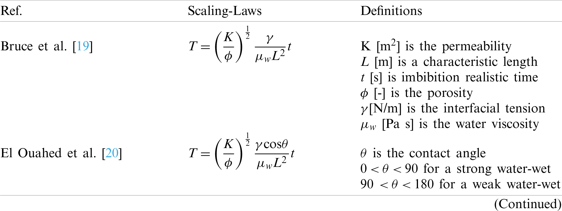
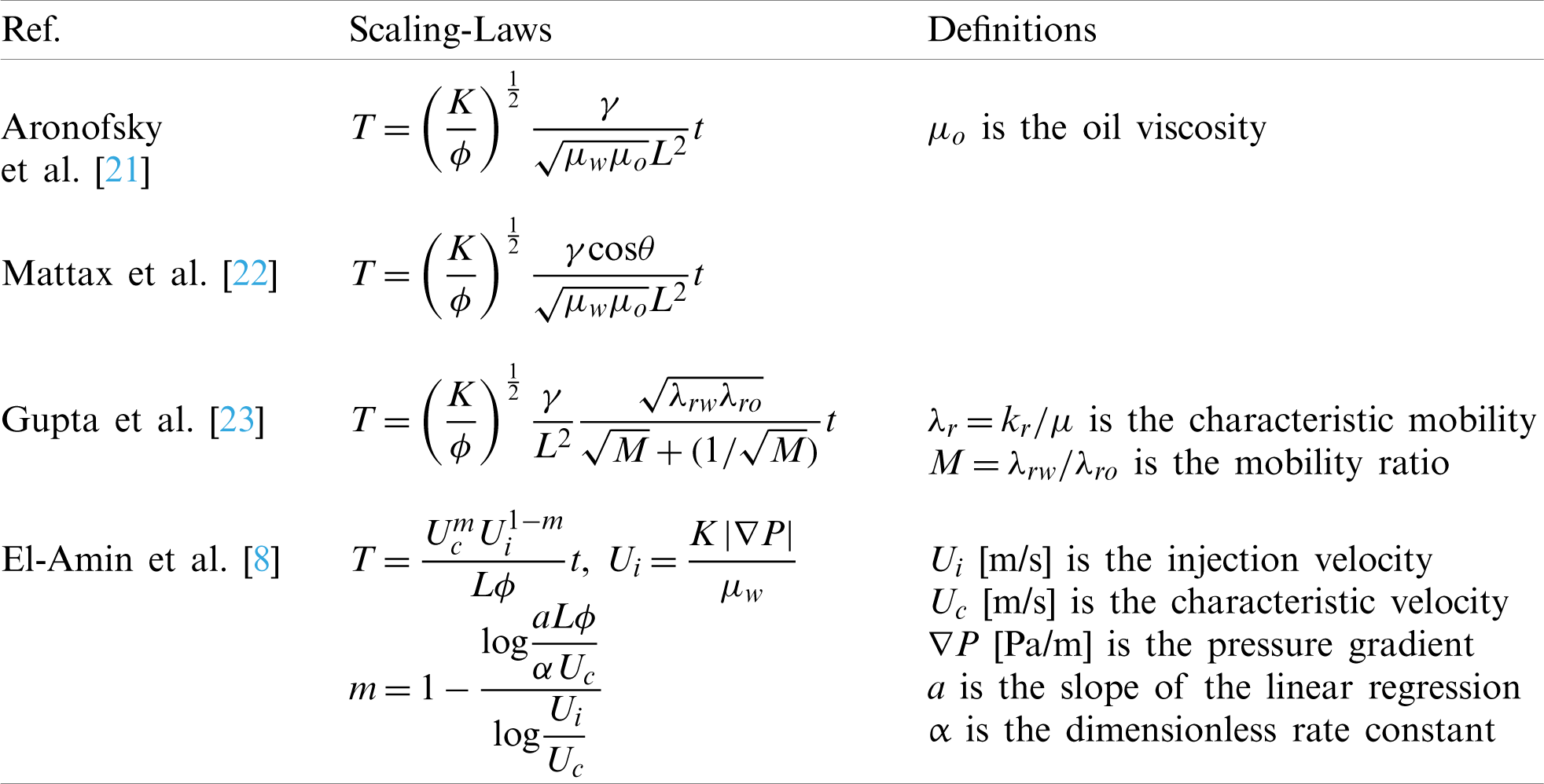
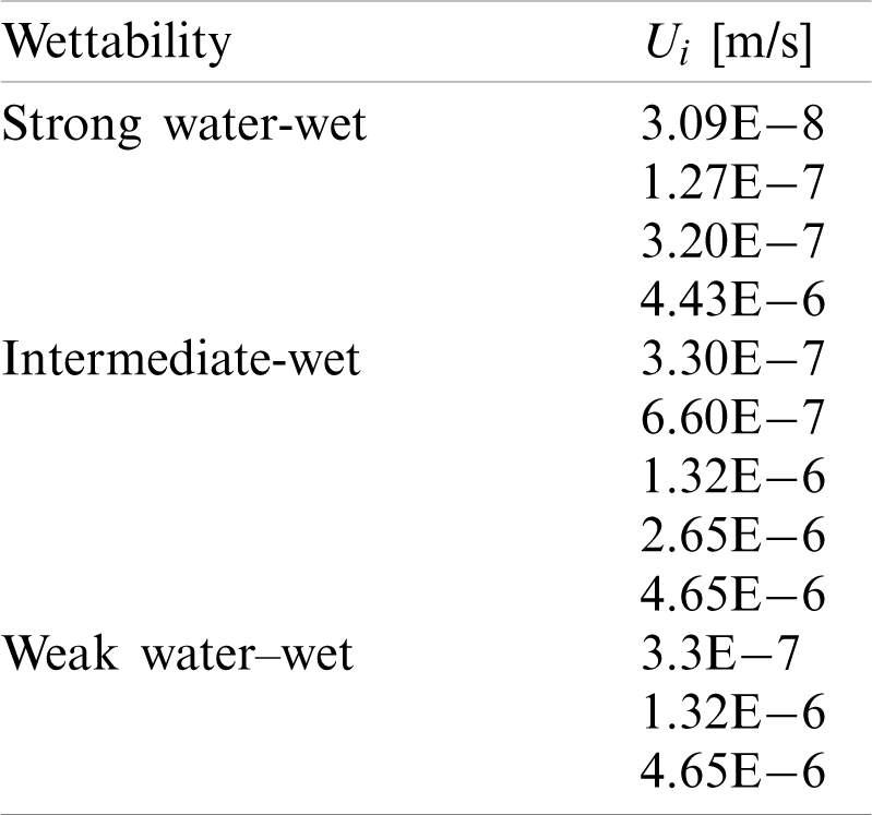
The generalized formula of dimensionless time by El-Amin et al. [8], contains spontaneous and forced imbibition cases. For example, for the countercurrent imbibition (m = 1), the scaling-law collapses to the other above formulas as those in Tab. 1. The velocity can be represented in terms of the given rock characteristics as shown in Tab. 2 for different wettability cases.

In the following subsections, selected machine learning methods have been presented including k-NN, ANNs, SVM, RF and SGB.

The k-NN is a nonparametric technique that can be utilized for classification and regression [24]. In k-NN regression, the nearest examples of functional training space represent the input, while the output is a property values average of the nearest neighbors of the object. Also, the k-NN is instance-based lazy learning, which approximates the function locally delays all computation after classification. This method can be utilized to give weight to the contributions of neighbors. Thus, neighbors contribute more to the average distance. For example, the typical weight for a given neighbor distance d is 1/d [24]. The neighborhood includes a set of objects with known property values that can represent the algorithm training set.

The idea of ANNs is to mimic the human brain’s task of learning from experience and then identify predictive patterns [25]. The neural network architecture generates nodes representing neurons and linking nodes matching axons, dendrites, and synapses. The ANN includes an input layer, an output layer, and a hidden layer. The input layer transforms the input variables, while the output layer transforms variables of the target. The input data gave by input nodes can achieve prediction. The input data is weighted by the links to the neural network’s values. A hidden layer uses a particular transfer function, and the forecast is calculated at the output nodes. With an additional recursive effort, ANN accumulates its predictive power. In a real sense, the network learns such that the learning examples are delivered to the network one by one. Nevertheless, the algorithms of the predictive model are close to other statistical methods. In a more straightforward sense, neural networks could be defined as a mixture of regression and general multivariate techniques. The architecture of the neural network was constructed from a multi-layer perspective. One may differentiate between the development of the model forward and backward spread. The method of backward propagation is commonly employed. ANNs can be described as a mixture of various multivariate forecast models in theoretical terms. However, the results are usually very complex and not instinctually simple. This approach is complex with simple, intermediate stages and intuitively consistent tests compared to regression and decision tree modeling. ANN was trained with 50 neurons in the hidden layer, 0.3 learning rate, 0.2 momentum value, and backpropagation algorithm.

The SVM (Support Vector Machine) method is linear/nonlinear data classification algorithms [26]. The SVM algorithm utilizes a nonlinear mapping to transform the original training data to a higher dimension. In general, the data is divided into two groups by hyperplane, which is created by a nonlinear mapping to a high dimension space. The SVM seeks the hyperplane by margins and support vectors. SVMs are reliable since they can predict complex nonlinear boundaries of decision; however, their training times are prolonged. SVMs are less sensitive than other algorithms to overfit. Linear SVMs cannot be utilized for linearly inseparable data. The linear SVM can be extended to contain nonlinear SVM for linearly inseparable data. Nonlinear SVMs allocate input space to nonlinear boundaries of decision (i.e., nonlinear hypersurfaces). Two main steps are introduced to get a nonlinear SVM. Such steps generate a quadratic optimization problem that a linear formulation of SVM can solve. SVM was trained with puk kernel with C=100.

The tree classifiers group, which is relevant to random vectors, is called random forest (RF) [27]. Assuming that a given training data of the random vector, {Vi: i=1,…,s} is and identically distributed and independent, a decision tree can be built with a classification model. This classification model has the highest voting classifier for the DT collection, {Mi: i=1,…,s}. On the other hand, the RF contains various decision trees’ ensemble schemes (e.g., bagging). The random vectors can match the number of the elements directly in the data set of the training object index, i.e., point to the successive bootstrap elements. Several sources like data sampling training or various decision configuration tree inducer consider the randomization of trees, which make up forests [28].

Grabczewski [29] implemented bagging techniques with the idea that they could improve their performance by introducing a type of randomness to the function of estimation procedures. Also, Breiman [30] have used random sampling boost implementations. However, it was deliberated to approximate stochastic weighting until the implementation of the base learner did not retain the observation weights. Freund et al. [31] recently proposed a hybrid adaptive bagging technique that replaces the base learner with the bagged base learner and replaces residuals “out of the bag” at each boosting step. Freund et al. [31] prompted a small shift to gradient boosting to incorporate uncertainty as an essential process metric. A minor change was inspired by gradient boosting to integrate uncertainty as a critical measure of the process. Moreover, the SGB scheme has been developed to be related to bagging and boosting [32–34]. The SBG technique has been applied in different fields, such as remote sensing problems [35]. The SBG was used by Moisen et al. [36] to predict the existence of species and basal area for 13 tree species.

The dataset and input variables used in this study were mainly experimental data extracted from many published papers [8,22,23,37–42]. The predicted values are typically the oil recovery and dimensionless time.

It is well known that an independent test set is not a good indicator of performance on the training set. One may use a training set based on each instance’s classifications within the training set. In order to predict a classifier’s performance on new data, an error estimation is required on a dataset (called test set), which has no role in classifier formation. The training data, as well as the test data, are assumed to be representative samples. In some particular cases, we have to differentiate between the test data and training data. It is worth mentioning that the test data cannot be utilized to generate the classifier. In general, there are three types of datasets, namely, training, validation, and test data. One or more learning schemes use the training data to create classifiers. The validation data is often employed to modify specific classifier parameters or to pick a different one. The test data will then be used to estimate the error of the final optimized technique. In order to obtain good performance, the training and testing sets should be chosen independently. Thus, in order to achieve better performance, the test set should be different from the training set. In many cases, the test data are manually classified, which reduces the number of the used data. A subset of data, which is called the holdout procedure, is used for testing, and the rest is employed for training, and sometimes a part can be used for validation [43]. In this study, 2/3 of the data is utilized for training, and 1/3 is used for testing.

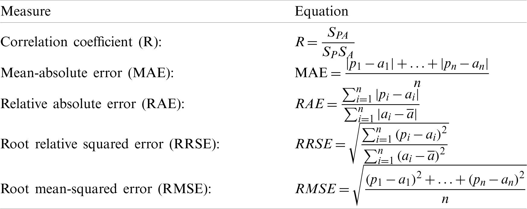
In order to evaluate the quality of each ML technique, a number of statistical measures are listed in Tab. 3. These measures include correlation coefficient (R), mean-absolute error (MAE), relative-absolute error (RAE), root relative squared error (RRSE) and root-mean-squared error (RMSE) [44–46]. For n test cases, assuming that the actual values ai and the predicted ones pi for the test case i are defined as:

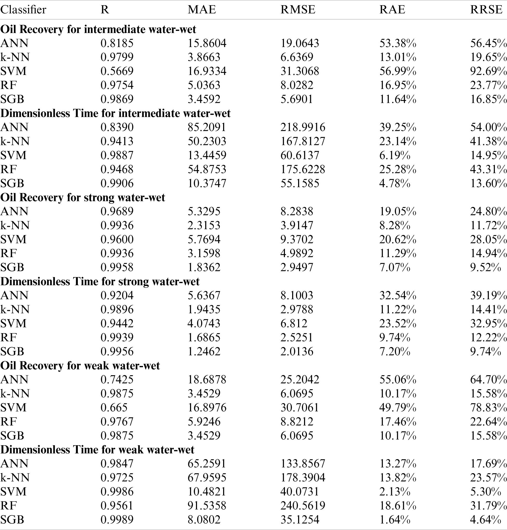
In this study, several machine learning algorithms are utilized to forecast the dimensionless time and oil recovery in terms of primary physical parameters of rocks and fluids. In this regard, diverse prediction models are developed, and the predictors’ performance is examined. As shown in Tab. 4, the SGB learner has achieved better efficiency than the ANN, k-NN, SVM, and RF.

Table 4: Performance of different ML techniques to predict oil recovery and nondimensional time for different wettability conditions

Figs. 2–4 demonstrate the predicted dimensionless time and oil recovery by the SGB model against the scaling-law (actual) ones [8] for strong/weak/intermediate water-wet cases. The findings show that the performance is enhanced with respect to the coefficient of correlation and MAE and less improvement with regard to RMSE, RAE, and RRSE. It is clearly observed that the SGB method has the highest correlation coefficient. Consequently, one may observe that the SVM method can be reliable in predicting both the oil recovery and dimensionless time because of its ability to achieve better performance while ensuring a better generalization.

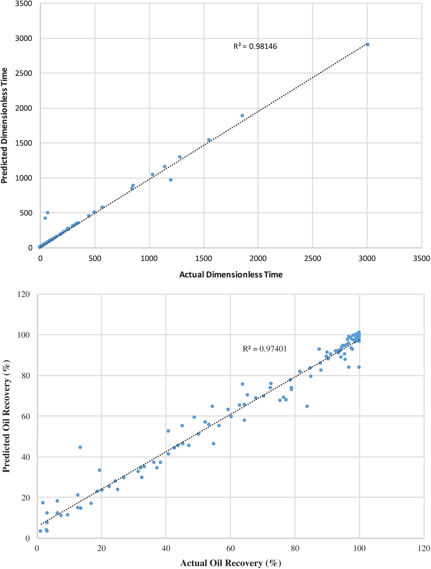
Figure 2: SGB predicted oil recovery and dimensionless time against actual scaling-law ones at for intermediate water-wet

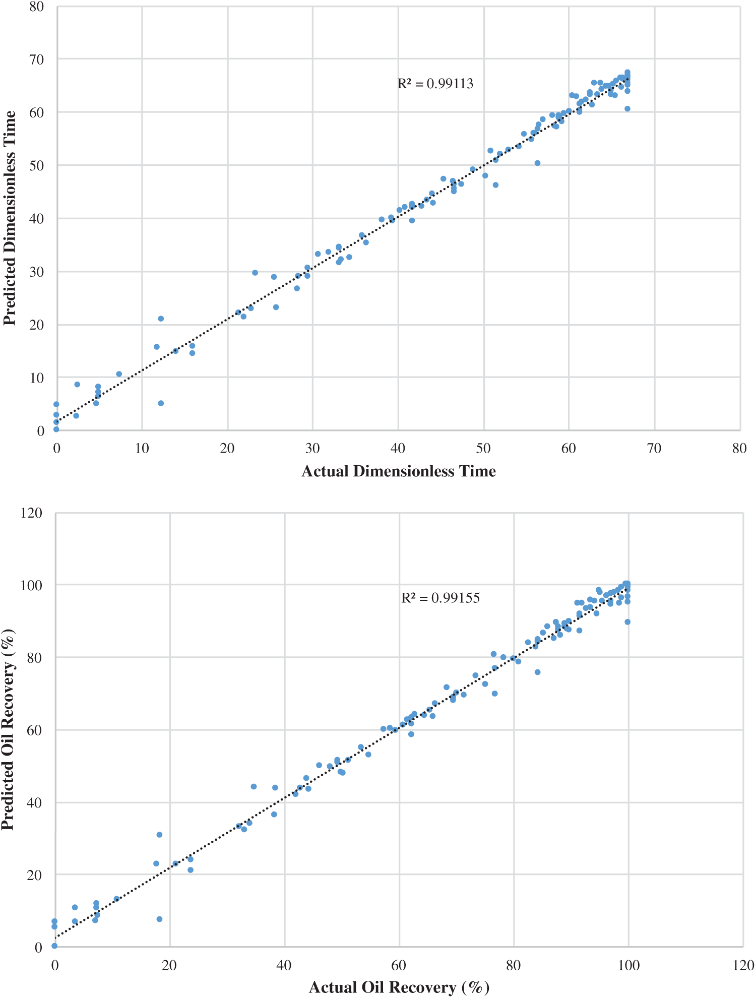
Figure 3: SGB predicted oil recovery and dimensionless time against actual scaling-law ones at for

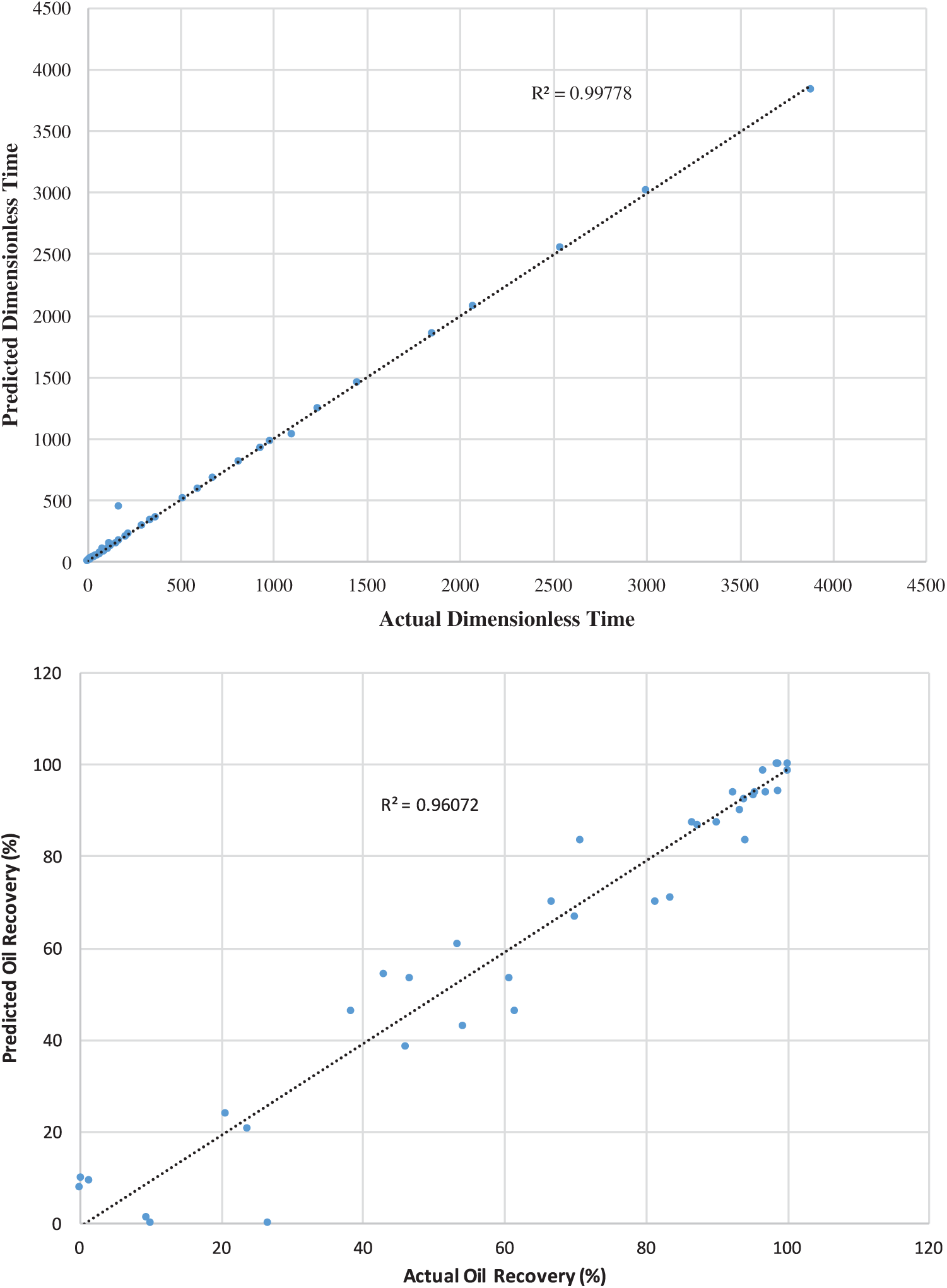
Figure 4: SGB predicted oil recovery and dimensionless time against actual scaling-law ones for weak water–wet

In this work, selected ML techniques have been used to predict the dimensionless time and oil recovery. So, several machine learning techniques are developed to predict the dimensionless time and oil recovery against the scaling-law (actual) ones for strong/weak/intermediate water-wet cases. When comparing the SGB algorithm with other techniques (Tab. 4), it achieved better performance than the ANN, k-NN, SVM, and RF regarding the correlation coefficient R and the RMS error. It is clear from this table that the RMS error of the SGB technique is smaller than those of other methods. Regarding the computational aspect, the SGB model requires a comparable complexity for the prediction compared to that of the ANN, SVM, and RF models. Unbiased tests can be used to evaluate the prediction performance of the used ML method. To test the accuracy of predictions, we quantify standard metrics such as coefficient of correlation (R) and error between the real and expected values. The experimental results have shown that the SGB technique can accurately evaluate the dimensionless time and oil recovery since it achieved a high value of R and low error. These models’ error and R assign the higher positive relationship between the expected and real oil recovery values. The results indicate increased performance in terms of correlation coefficient and MAE and rose ultimately with RMSE, RAE, and RRSE.

If one compares the performances of the machine learning techniques for the predicted dimensionless time and oil recovery against the scaling-law (actual) ones for strong/weak/intermediate water-wet cases, the proposed SGB method achieved the best results in all cases. But, ANN, k-NN, SVM, and RF are also accomplished good performance in some cases. For instance, SGB achieved R = 0.9869, MAE = 3.4592 and RMSE = 5.6901, k-NN is also achieved similar results with R = 0.9799, MAE = 3.8663, and RMSE = 6.6369 for oil recovery in the intermediate water-wet case. SGB achieved R = 0.9906, MAE = 10.3747 and RMSE = 55.1585, SVM is also achieved similar results with R = 0.9887, MAE = 13.4459 and RMSE = 60.6137 for dimensionless time in the intermediate water-wet case. SGB achieved R = 0.9958, MAE = 1.8362 and RMSE = 2.9497, k-NN is also achieved similar results with R = 0.9936, MAE = 2.3153 and RMSE = 3.9147 for oil recovery in the strong water–wet case. SGB achieved R = 0.9956, MAE = 1.2462 and RMSE = 2.0136. Random Forest is also achieved similar results with R = 0.9939, MAE = 1.6865, and RMSE = 2.5251 for the dimensionless time in the strong water-wet case. SGB achieved R = 0.9875, MAE = 3.4529 and RMSE = 6.0695, k-NN is also achieved the same results with R = 0.9875, MAE = 3.4529, and RMSE = 6.0695 for oil recovery in the weak water–wet case. SGB achieved R = 0.9989, MAE = 8.0802 and RMSE = 35.1254, SVM is also achieved the similar results with R = 0.9986, MAE = 10.4821 and RMSE = 40.0731 for dimensionless time in the weak water–wet case. In all cases, the SGB model outperformed the other models. This reveals that the SGB is a robust model and tackle well noisy conditions. The overall results illustrate that the SGB technique can effectively handle the expected oil recovery data because of its ability to produce better performance while ensuring better generalization.

As the dimensionless scaled-time law is fundamental to predict oil-recovery using laboratory data. We examined several ML techniques (k-NN, ANN, SVM, RF, and SBG) to predict the dimensionless scaling-law based on oil and rock physical properties in the current paper. The SGB regression was found to be the best ML method for predicting dimensionless scaling-time. The machine learning techniques’ performance has been compared using R, MAE, RMSE, RAE, and RRSE. Assessment of the experimental results among the machine learning techniques has shown that the SGB algorithm has the best prediction performance. Besides, the SGB model achieved higher prediction accuracy and lowered MAE, RMSE, RAE, and RRSE compared to k-NN, ANN, SVM, and RF regression models.

Conflicts of Interest: The authors declare that they have no conflicts of interest to report regarding the present study.

References

B. J. Bourbiaux and F. J. Kalaydjian, “Experimental study of cocurrent and countercurrent flows in natural porous media,” SPE Reservoir Engineering, vol. 5, no. 3, pp. 361–368, 1990.
M. E. Chimienti, S. N. Illiano and H. L. Najurieta, “Influence of temperature and interfacial tension on spontaneous imbibition process,” in Proc. Latin American and Caribbean Petroleum Engineering Conf., SPE-53668-MS, Caracas, Venezuela, 1999.
M. Pooladi-Darvish and A. Firoozabadi, “Co-current and countercurrent imbibition in a water-wet matrix block,” SPE Journal, vol. 5, no. 1, pp. 3–11, 2000.
H. L. Najurieta, N. Galacho, M. E. Chimienti and S. N. Illiano, “Effects of temperature and interfacial tension in different production mechanisms,” in Proc. Latin American and Caribbean Petroleum Engineering Conf., SPE-69398-MS, Buenos Aires, Argentina, 2001.
G. Tang and A. Firoozabadi, “Effect of pressure gradient and initial water saturation on water injection in water-wet and weak water–wet fractured porous media,” SPE Reservoir Evaluation & Engineering, vol. 4, no. 6, pp. 516–524, 2001.
M. F. El-Amin and S. Sun, “Effects of gravity and inlet/outlet location on a two-phase co-current imbibition in porous media,” Journal of Applied Mathematics, vol. 2011, pp. 673523, 2011.
M. F. El-Amin, A. Salama and S. Sun, “Numerical and dimensional investigation of two-phase countercurrent imbibition in porous media,” Journal of Computational and Applied Mathematics, vol. 242, no. 2, pp. 285–296, 2013.
M. F. El-Amin, A. Salama and S. Sun, “A generalized power-law scaling law for a two-phase imbibition in a porous medium,” Journal of Petroleum Science and Engineering, vol. 111, no. 4, pp. 159–169, 2011.
M. Tusiani and G. Shearer, LNG: A Nontechnical Guide, Tulsa, Oklahoma, US: PennWell Group, 2007.
S. O. Olatunji, A. Selamat and A. A. Abdul Raheem, “Predicting correlations properties of crude oil systems using type-2 fuzzy logic systems,” Expert Systems with Applications, vol. 38, no. 9, pp. 10911–10922, 2011.
K. O. Akande, T. O. Owolabi and S. O. Olatunji, “Investigating the effect of correlation-based feature selection on the performance of support vector machines in reservoir characterization,” Journal of Natural Gas Science and Engineering, vol. 22, no. 5, pp. 515–522, 2015.
S. Elkatatny, M. Mahmoud, Z. Tariq and M. Abdulraheem, “New insights into the prediction of heterogeneous carbonate reservoir permeability from well logs using artificial intelligence network,” Neural Computing and Applications, vol. 30, no. 9, pp. 2673–26883, 2018.
S. Karimpouli, N. Fathianpour and J. Roohi, “A new approach to improve neural networks’ algorithm in permeability prediction of petroleum reservoirs using supervised committee machine neural network (SCMNN),” Journal of Petroleum Science and Engineering, vol. 73, no. 3–4, pp. 227–232, 2010.
R. Gholami, A. Shahraki and M. J. Paghaleh, “Prediction of hydrocarbon reservoirs permeability using support vector machine,” Mathematical Problems in Engineering, vol. 2012, no. 23, pp. 1–18, 2012.
A. Subasi, M. F. El-Amin, T. Darwich and T. Al Dosary, “Permeability prediction of petroleum reservoirs using stochastic gradient boosting regression,” Journal of Ambient Intelligence and Humanized Computing, vol. 22, no. 6, pp. 515, 2020.
M. F. El-Amin and A. Subasi, “Forecasting a small-scale hydrogen leakage in air using machine learning techniques,” in Proc. 2020 2nd Int. Conf. on Computer and Information Sciences, Aljouf, Saudi Arabia, 2020.
M. F. El-Amin and A. Subasi, “Predicting turbulent buoyant jet using machine learning techniques,” in Proc. 2020 2nd Int. Conf. on Computer and Information Sciences, Aljouf, Saudi Arabia, 2020.
P. Wong, F. Aminzadeh and M. Nikravesh, “Soft computing for reservoir characterization and modeling,” in Series: Studies in Fuzziness and Soft Computing. vol. 80, Berlin, Germany: Springer, 2013.
A. Bruce, P. Wong, Y. Zhang, H. Salisch, C. Fung et al., “A state-of-the-art review of neural networks for permeability prediction,” APPEA Journal, vol. 40, no. 1, pp. 341–354, 2000.
A. K. El Ouahed, D. Tiab and A. Mazouzi, “Application of artificial intelligence to characterize naturally fractured zones in Hassi Messaoud oil field,” Algeria Journal of Petroleum Science and Engineering, vol. 49, no. 3–4, pp. 122–141, 2005.
J. S. Aronofsky, L. Masse and S. G. Natanson, “A model for the mechanism of oil recovery from the porous matrix due to water invasion in fractured reservoirs,” Transactions of the AIME, vol. 213, no. 1, pp. 17–19, 1958.
C. C. Mattax and J. R. Kyte, “Imbibition oil recovery from fractured water drive reservoir,” SPE Journal, vol. 2, pp. 177–184, 1962.
A. Gupta and F. Civan, “An improved model for laboratory measurement of matrix to fracture transfer function parameters in immiscible displacement,” in Proc. of the SPE Annual Technical Conf. and Exhibition, New Orleans, Los Angeles, USA, 1994.
S. Ma, N. R. Morrow, R. N. and X. Zhang, “Generalized scaling of spontaneous imbibition data for strong water-wet systems,” Journal of Petroleum Science and Engineering, vol. 18, no. 3-4, pp. 165–178, 1997.
N. S. Altman, “An introduction to kernel and nearest-neighbor nonparametric regression,” American Statistician, vol. 46, no. 3, pp. 175–185, 1992.
A. Ahlemeyer-Stubbe and S. Coleman, “A practical guide to data mining for business and industry,” in Data Mining Statistics. Hoboken, New Jersey, United States: John Wiley & Sons, 2014.
J. Han, J. Pei and M. Kamber, Data Mining: Concepts and Techniques, Amsterdam, Netherlands: Elsevier, 2011.
L. Breiman, “Random forests,” Machine Learning, vol. 45, no. 1, pp. 5–32, 2001.
K. Grabczewski, “Meta-learning in decision tree induction,” in Studies in Computational Intelligence. vol. 1, Berlin, Germany: Springer, 2014.
L. Breiman, “Bagging predictors,” Machine Learning, vol. 24, no. 2, pp. 123–140, 1996.
Y. Freund and R. E. Schapire, “A decision-theoretic generalization of on-line learning and an application to boosting,” Journal of Computer and System Sciences, vol. 55, no. 1, pp. 23–37, 1995.
L. Breiman, “Using adaptive bagging to debias regressions,” Technical Report 547, Statistics Department UCB, 1999.
J. H. Friedman, “Greedy function approximation: A gradient boosting machine,” Annals of Statistics, vol. 29, no. 5, pp. 1189–1232, 2001.
J. H. Friedman, “Stochastic gradient boosting,” Computational Statistics & Data Analysis, vol. 38, no. 4, pp. 367–378, 2002.
G. Ridgeway, “The state of boosting,” Computing Science and Statistics, vol. 31, pp. 172–181, 1999.
G. G. Moisen, E. A. Freeman, J. A. Blackard, T. S. Frescino, N. E. Zimmermann et al., “Predicting tree species presence and basal area in Utah: A comparison of stochastic gradient boosting, generalized additive models, and tree-based methods,” Ecological Modelling, vol. 199, no. 2, pp. 176–187, 2006.
G. Hamon and J. Vidal, “Scaling-up the capillary imbibition process from laboratory experiments on homogeneous samples,” in Proc. the 1986 SPE European Petroleum Conf., London, pp. 22–25, 1986.
T. Babadagli, “Scaling of capillary imbibition during static thermal and dynamic fracture flow conditions,” Journal of Petroleum Science and Engineering, vol. 33, no. 4, pp. 223–239, 1997.
T. Babadagli, “Scaling of concurrent and countercurrent capillary imbibition for surfactant and polymer injection in naturally fractured reservoir,” SPE Journal, vol. 6, no. 4, pp. 465–478, 2001.
Z. Tong, X. Xie and R. N., “Morrow Scaling of viscosity ratio and oil recovery by imbibition from mixed-wet rocks,” in Proc. Int. Symp. of the Society of Core Analysis, Edinburgh, SCA 2001–21, UK, 2001.
Z. Tavassoli, R. W. Zimmerman and M. J. Blunt, “Analytic analysis of oil recovery during countercurrent imbibition in strong water–wet system,” Transport in Porous Media, vol. 58, no. 1–2, pp. 173–189, 2005.
K. Li, “Scaling of spontaneous imbibition data with wettability included,” Journal of Contaminant Hydrology, vol. 89, no. 3–4, pp. 218–230, 2007.
I. Witten, E. Frank and M. Hall, “Data mining: Practical machine learning tools and techniques,” in The Morgan Kaufmann Series in Data Management Systems, 3rd ed. Burlington: Kaufmann, 2011.
S. O. Olatunji, A. Selamat and A. Abdulraheem, “A hybrid model through the fusion of type-2 fuzzy logic systems and extreme learning machines for modelling permeability prediction,” Information Fusion, vol. 16, pp. 29–45, 2014.
S. Cankurt and A. Subasi, “Tourism demand modelling and forecasting using data mining techniques in multivariate time series: A case study in Turkey,” Turkish Journal of Electrical Engineering and Computer Sciences, vol. 24, no. 5, pp. 3388–3404, 2016.
V. Ülke, A. Sahin and A. Subasi, “A comparison of time series and machine learning models for inflation forecasting: Empirical evidence from the USA,” Neural Computing and Applications, vol. 30, no. 5, pp. 1519–1527, 2018.

Computers, Materials & Continua DOI:10.32604/cmc.2021.017102
Article