DOI:10.32604/cmc.2021.017410
| Computers, Materials & Continua DOI:10.32604/cmc.2021.017410 | |
| Article |
Deep-Learning-Empowered 3D Reconstruction for Dehazed Images in IoT-Enhanced Smart Cities
1Tamoritsusho Co., Ltd., Tokyo, 110-0005, Japan
2Global Information and Telecommunication Institute, Waseda University, Tokyo, 169-8050, Japan
3School of Fundamental Science and Engineering, Waseda University, Tokyo, 169-8050, Japan
*Corresponding Author: Xin Qi. Email: samqixin@aoni.waseda.jp
Received: 29 January 2021; Accepted: 01 March 2021
Abstract: With increasingly more smart cameras deployed in infrastructure and commercial buildings, 3D reconstruction can quickly obtain cities’ information and improve the efficiency of government services. Images collected in outdoor hazy environments are prone to color distortion and low contrast; thus, the desired visual effect cannot be achieved and the difficulty of target detection is increased. Artificial intelligence (AI) solutions provide great help for dehazy images, which can automatically identify patterns or monitor the environment. Therefore, we propose a 3D reconstruction method of dehazed images for smart cities based on deep learning. First, we propose a fine transmission image deep convolutional regression network (FT-DCRN) dehazing algorithm that uses fine transmission image and atmospheric light value to compute dehazed image. The DCRN is used to obtain the coarse transmission image, which can not only expand the receptive field of the network but also retain the features to maintain the nonlinearity of the overall network. The fine transmission image is obtained by refining the coarse transmission image using a guided filter. The atmospheric light value is estimated according to the position and brightness of the pixels in the original hazy image. Second, we use the dehazed images generated by the FT-DCRN dehazing algorithm for 3D reconstruction. An advanced relaxed iterative fine matching based on the structure from motion (ARI-SFM) algorithm is proposed. The ARI-SFM algorithm, which obtains the fine matching corner pairs and reduces the number of iterations, establishes an accurate one-to-one matching corner relationship. The experimental results show that our FT-DCRN dehazing algorithm improves the accuracy compared to other representative algorithms. In addition, the ARI-SFM algorithm guarantees the precision and improves the efficiency.
Keywords: 3D reconstruction; dehazed image; deep learning; fine transmission image; structure from motion algorithm
Artificial intelligence (AI) has recently become very popular, and a wide range of applications use this technique [1]. There are many smart systems based on deep learning for social services, such as smart cities and smart transportation. Smart cities can use AI technology such as machine learning, deep learning and computer vision to save money and improve the quality of life of residents [2]. Through using AI or machine learning technology to perform intelligent image processing, we can obtain important geographical region data. Such real-time data can be continuously monitored through AI technology, which would further develop cities’ governance and planning [3].
In hazy environments, the reflected light of an object is attenuated before it reaches the camera or monitoring equipment, resulting in the degradation of the quality of an outdoor image [4]. Therefore, obtaining dehazed images in smart cities is an important problem to be solved by AI technology. In recent years, with the rapid development of AI technology, some dehazing algorithms based on deep learning have been proposed. Tang et al. [5] used the random forest algorithm to remove haze. Although the accuracy of the transmission image was improved, the texture features in the image were not used, which has certain limitations; and the effect of dehazing is not ideal. Cai et al. [6] adopted the convolutional neural network to learn the features of hazy image to estimate the transmission image. The convolutional neural network only uses a single scale for feature extraction, which makes it prone to color distortion, detail loss and excessive dehazing for many specific scenes. Li et al. [7] proposed AOD-Net based on a convolutional neural network to dehaze images. To avoid using additional methods to estimate atmospheric light via mathematical transformation, the network structure of this algorithm is relatively simple.
We propose a fine transmission image deep convolutional regression network (FT-DCRN) dehazing algorithm that uses fine transmission image [8] and atmospheric light value [9] to compute dehazed image. First, this paper proposes a deep convolutional regression network (DCRN) to obtain the coarse transmission image. The DCRN can not only expand the receptive field of the network, but it can also retain the features to maintain the nonlinearity of the overall network [10]. Second, the fine transmission image is obtained by refining the coarse transmission image using a guided filter [11]. The guided filter is used to optimize the coarse transmission image to improve the accuracy of dehazed images. Furthermore, the atmospheric light value is estimated according to the position and brightness of the pixels in the original hazy image. According to the obtained fine transmission image and atmospheric light value, the dehazed image is inverted using the atmospheric physical scattering model [12].
With increasingly more smart cameras deployed in infrastructure and commercial buildings, 3D reconstruction can quickly obtain information on cities and geographical regions [13]. It is important to solve the image matching problem using structure from motion (SFM) 3D reconstruction algorithms [14]. Feature detection and feature matching are subordinate image matching problems. Hossain et al. [15] proposed a CADT corner detection algorithm, which effectively reduces the positioning error and improves the average repeatability. Zhang et al. [16] proposed a Harris SIFT algorithm including illumination compensation, which not only improves the matching accuracy but also improves the real-time performance of the algorithm. However, the above image matching algorithms are not universal and cannot accurately extract image feature points under special lighting conditions. Zhou et al. [17] proposed a registration algorithm based on geometric invariance and local similar features, but it relies heavily on rough matching, and the correct matching points are eliminated. To solve the problems of the above algorithms, an advanced relaxed iterative fine matching based on the SFM (ARI-SFM) algorithm is proposed. The ARI-SFM algorithm, which obtains the fine matching corner pairs and reduces the number of iterations, establishes an accurate one-to-one corner matching relationship.
The contributions of this paper are listed as follows:
a) We use a deep learning algorithm for dehazed images in smart cities. The FT-DCRN dehazing algorithm is proposed, which uses fine transmission image and atmospheric light value to compute dehazed image. First, this paper proposes a DCRN algorithm to obtain the coarse transmission image. The DCRN can not only expand the receptive field of the network, but can also retain the features to maintain the nonlinearity of the overall network. Second, the fine transmission image is obtained by refining the coarse transmission image using a guided filter. The guided filter is used to optimize the coarse transmission image to improve the accuracy of dehazed images.
b) We perform 3D reconstruction using the dehazed images generated from the FT-DCRN algorithm. The ARI-SFM algorithm is proposed, which can obtain fine matching corner pairs and reduce the number of iterations. Compared with other representative algorithms, the ARI-SFM algorithm establishes an accurate one-to-one corner matching relationship, which guarantees the precision and improves the efficiency.
2.1 FT-DCRN Dehazing Algorithm
The purpose of a dehazing algorithm is to restore a sharp image from a blurred image caused by haze. Deep learning algorithms can provide great help for dehazy images [18], which can automatically identify patters or monitor the environment. In this paper, we propose a FT-DCRN dehazing algorithm to obtain useful images for 3D reconstruction. The steps of the FT-DCRN dehazing algorithm are as follows:
Step 1: Obtain the coarse transmission image. Input the hazy images, and the coarse transmission image is obtained by using the DCRN dehazing algorithm.
Step 2: Compute the fine transmission image. The fine transmission image is obtained by refining the coarse transmission image using a guided filter.
Step 3: Estimate the atmospheric light value. The atmospheric light value [19] is estimated according to the position and brightness of the pixels in the original hazy image.
Step 4: Compute the dehazed image. According to the obtained fine transmission image and atmospheric light value, the dehazed image is inverted using the atmospheric physical scattering model.
To obtain a coarse transmission image, this paper proposes a DCRN dehazing algorithm, and the overall network structure is shown in Fig. 1. The DCRN is an end-to-end network based on a convolutional neural network [20] that inputs hazy images and outputs corresponding coarse transmission images.
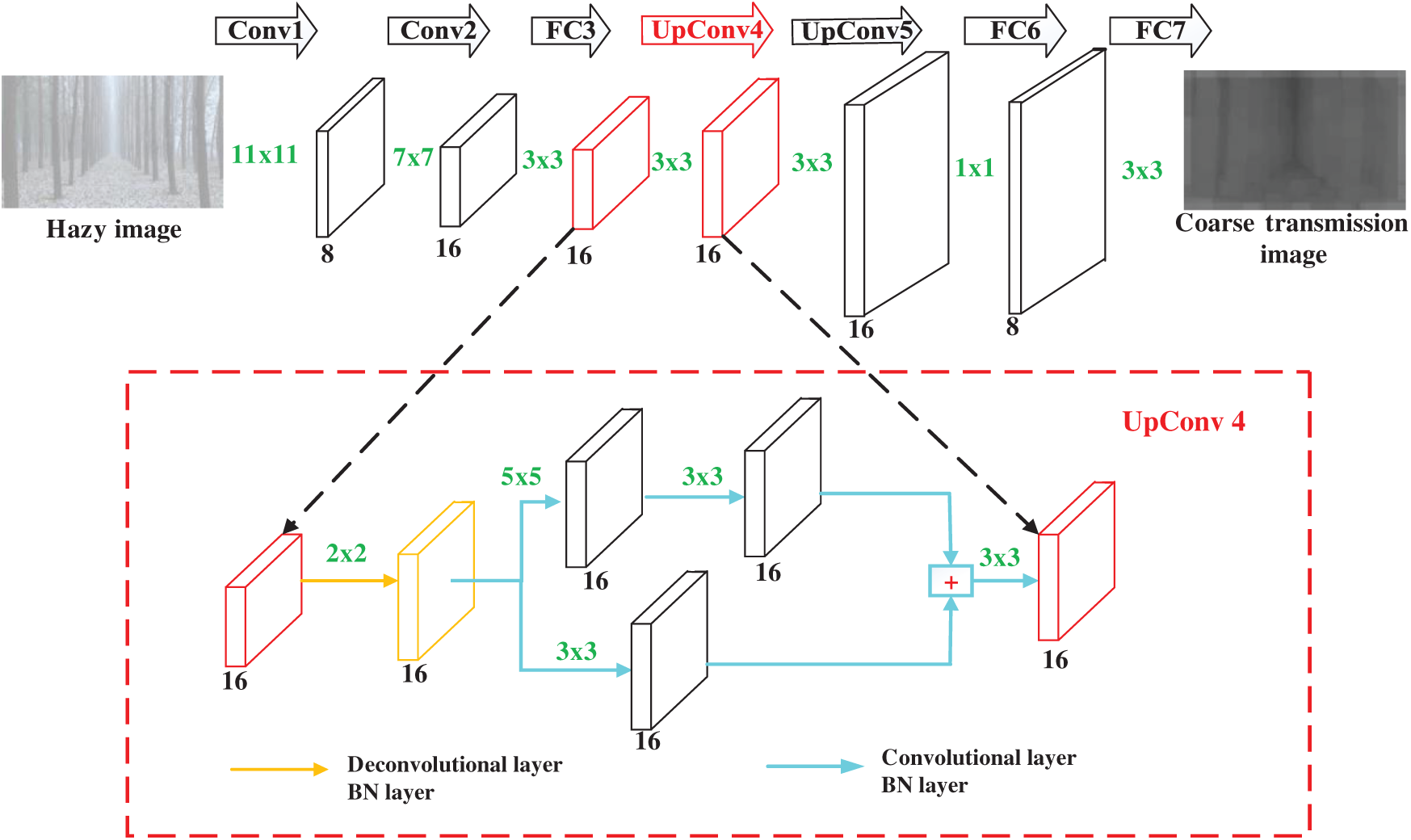
Figure 1: Overall network structure of DCRN dehazing algorithm
The DCRN is similar to the encoder–decoder network. The core unit of the encoder network is the convolutional unit (Conv), which is mainly composed of a convolutional layer [21], an ReLU, a pooling layer and a batch normalization (BN) layer [22]. The core unit of the decoder network is the deconvolutional unit (DeConv), which is mainly composed of a deconvolutional layer, a BN layer, an ReLU and a convolutional layer. The fully connected (FC) layer [23] is replaced by the convolutional layer.
The features of the overall network are extracted by the encoder network. The decoder network is used to ensure the size of the output transmission image and retain the features to maintain the nonlinearity of the overall network [24]. Our DCRN can not only expand the receptive field of the network, but it can also ensure that the overall network has a certain nonlinear learning ability.
The main characteristic of an end-to-end network is that the input and output of the network are identical in size. However, due to the use of two pooling layers [25] in the encoder network, the feature set is smaller, and the original image information is lost.
To solve the problem of information loss from the original image, this paper uses a deconvolutional layer [26] to replace the upsampling layer, which can not only increase the size of the feature set, but can also produce a dense feature set with a larger spatial structure, the “Upconv4” is shown in the red box of Fig. 1. The Upconv4 contains the deconvolutional layer, convolutional layer and BN layer. The deconvolutional layer is often used in the densest mapping estimation problem. Furthermore, the cross-convolutional layer used in the DeConv unit can not only provide the DCRN with the multiscale feature learning ability, but can also avoid the vanishing gradient problem in the backpropagation process. Therefore, the DCRN can estimate the coarse transmission image more accurately.
In this paper, a guided filter is used to optimize the coarse transmission image to improve the accuracy of dehazed images [27]. The guided filter can be defined as:
where q is the output image, which is the fine transmission image obtained after optimization. ak and bk are the coefficients of the window
where
where uk and
When estimating the atmospheric light value, He et al. [28] selected the pixels with the top one percent brightnesses in the hazy image and then calculated the average brightness of these pixels as the atmospheric light value. This method is more effective in most cases, but when a large white area appears in the image, the method will not accurately estimate the atmospheric light value, which will lead to image color distortion.
To solve the above problems, this paper uses the method of combining the pixel position and brightness to estimate the atmospheric light value. The relative height of each pixel is defined as
The process determines the pixels with the probability value
It is important to solve the image matching problem in the 3D SFM reconstruction algorithm. In the image matching process, the coarse matching relationship between corners is established by using the zero mean normalized cross-correlation method [29]. This method only builds a one-to-many set of matching corner pairs, so there are many unclear and incorrect matching pairs. We propose an ARI-SFM algorithm to guarantee the precision and improve the efficiency.
To establish an accurate one-to-one corner matching relationship, an advanced relaxed iterative (ARI) algorithm is proposed, which obtains fine matching corner pairs and reduces the number of iterations. The flowchart of the ARI algorithm is shown in Fig. 2.
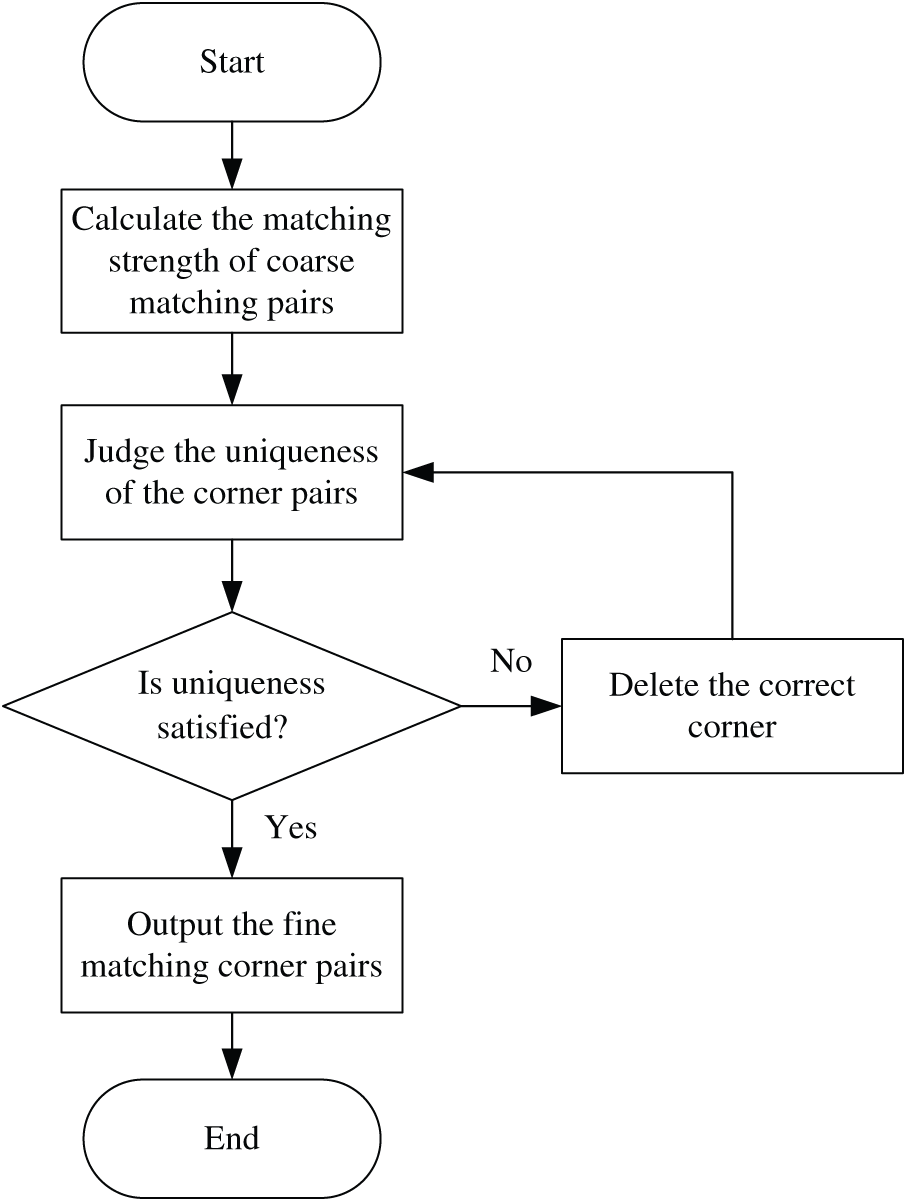
Figure 2: Flowchart of the ARI algorithm
The steps of the ARI algorithm are as follows:
Step 1: Calculate the matching strength of coarse matching pairs. The matching strength is used as the indicator for fine matching corner selection [30].
Step 2: Judge the uniqueness of the corner pairs. The matching pairs are sorted according to the matching strength from large to small. We select the corner pairs SM(p1i, q2j) and
The value range of SP is 0
Step 3: Delete the correct corner after fine matching, and return to Step 1.
Step 4: Output the fine matching corner pairs.
2.2.2 Calculation of Matching Strength
The initial matching corner pairs are represented as (p1i, q2j), where p1i is the corner of image I1 and q2j is the corner of image I2. N(p1i) and N(q2j) are neighborhoods with point p1i and point q2j as centers, respectively, and R as the radius. If (p1k, q2f) is the correct matching pair, there must be more correct matching pairs (p1k, q2f) in its neighborhoods
Condition 1: Only the matching corner pair (p1k, q2f) affects the matching corner pair (p1i, q2j).
Condition 2: The angle between
If the matching corner pairs (p1i, q2j) and (p1k, q2f) satisfy the above two conditions, the matching strength is calculated using formula (7):
r is the relative distance deviation of the corner pair. The similarity contribution
In this paper, synthetic hazy images and real hazy images are used to train and test the performance of the FT-DCRN dehazing algorithm. First, we adopt the Make3D dataset [31] (http://make3d.cs.cornell.edu/data.html) to synthesize hazy images using the atmospheric scattering model. We selected 900 pairs of hazy and sharp images as training samples. Second, we take 1200 real hazy images of outdoor scenes, such as those of buildings, gardens, and parking areas, to analyze the results of the FT-DCRN dehazing algorithm. The FT-DCRN dehazing algorithm runs on a GeForce RTX 2080Ti GPU and executes using Python.
To verify the efficiency and accuracy of the ARI-SFM algorithm, the algorithm is implemented on an experimental platform with 64-bit Windows 10, an Intel(R) Core(TM) i5-10210U@1.60 GHZ CPU, and 8.00 GB of memory; the development platform is MATLAB R2018b.
3.1 Generation of Synthetic Hazy Images
Given a random value for the transmission image
where
Fig. 3 shows the original sharp images, including images of a road, house, tree, and fountain, from the Make3D dataset. Fig. 4 shows the corresponding synthetic hazy image of the sharp images in the Make3D dataset.
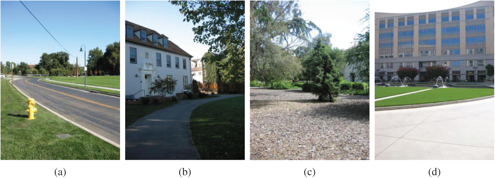
Figure 3: Original sharp images from the Make3D dataset. (a) Road. (b) House. (c) Tree. (d) Fountain
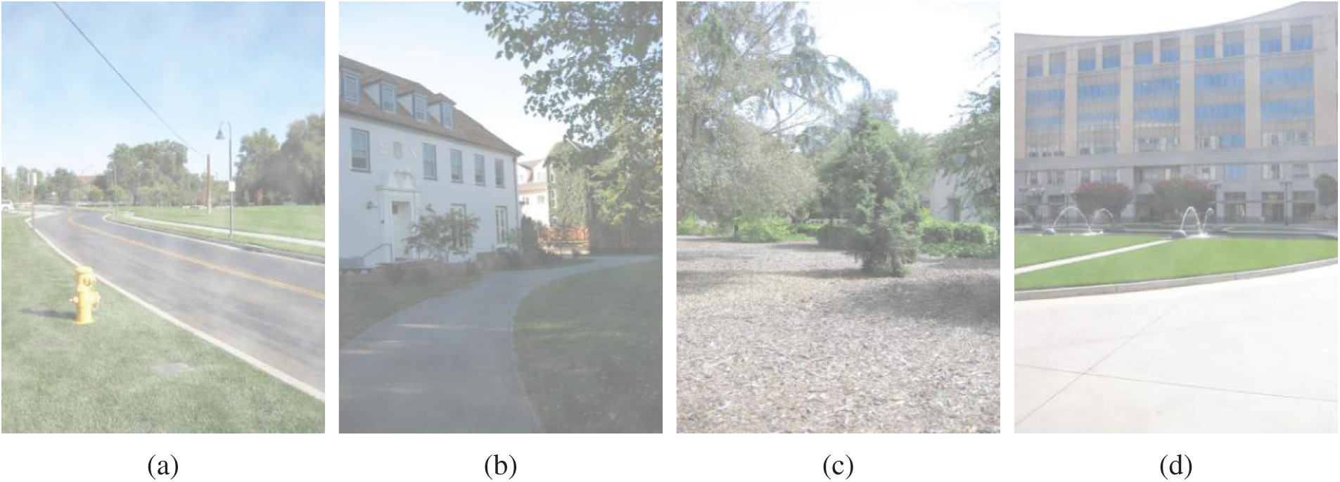
Figure 4: Corresponding synthetic hazy images from the Make3D dataset. (a) Road. (b) House. (c) Tree. (d) Fountain
3.2 Experiment of FT-DCRN Dehazing Algorithm
(1) Results of Synthetic Hazy Images
To verify the effect of the FT-DCRN dehazing algorithm on the synthetic hazy images, the results of the algorithm are compared with some representative algorithms. Because different deep learning algorithms have their own advantages,we adopt the Tang’s algorithm [5], Cai’s algorithm [6] and Li’s algorithm [7], which are described in the introduction. Figs. 5–8 show the comparison results of the dehazing of the road, house, tree and fountain images in the Make3D dataset.
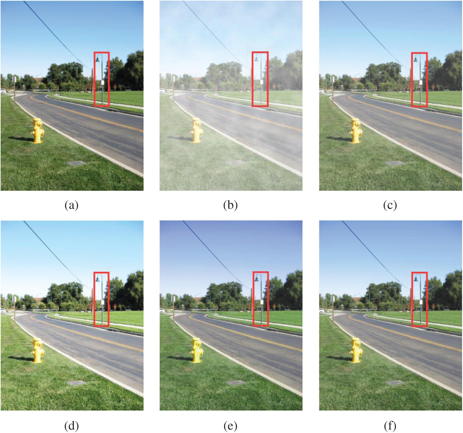
Figure 5: Comparison results of the dehazing of the road images. (a) Sharp image. (b) Synthetic hazy image. (c) Tang’s algorithm. (d) Cai’s algorithm. (e) Li’s algorithm. (f) Our approach
Figs. 5–8 show that Tang’s algorithm does not consider the texture features in the images, and the results of the algorithm have unclear boundaries. Cai’s algorithm has color oversaturation in dehazed images, resulting in large areas of color distortion. Li’s algorithm contains detailed information, but the overall colors of the images are not close to the normal visual effect. Our approach is superior to other methods. The boundaries of the dehazed images are clear, and the textures are close to those of the real images.
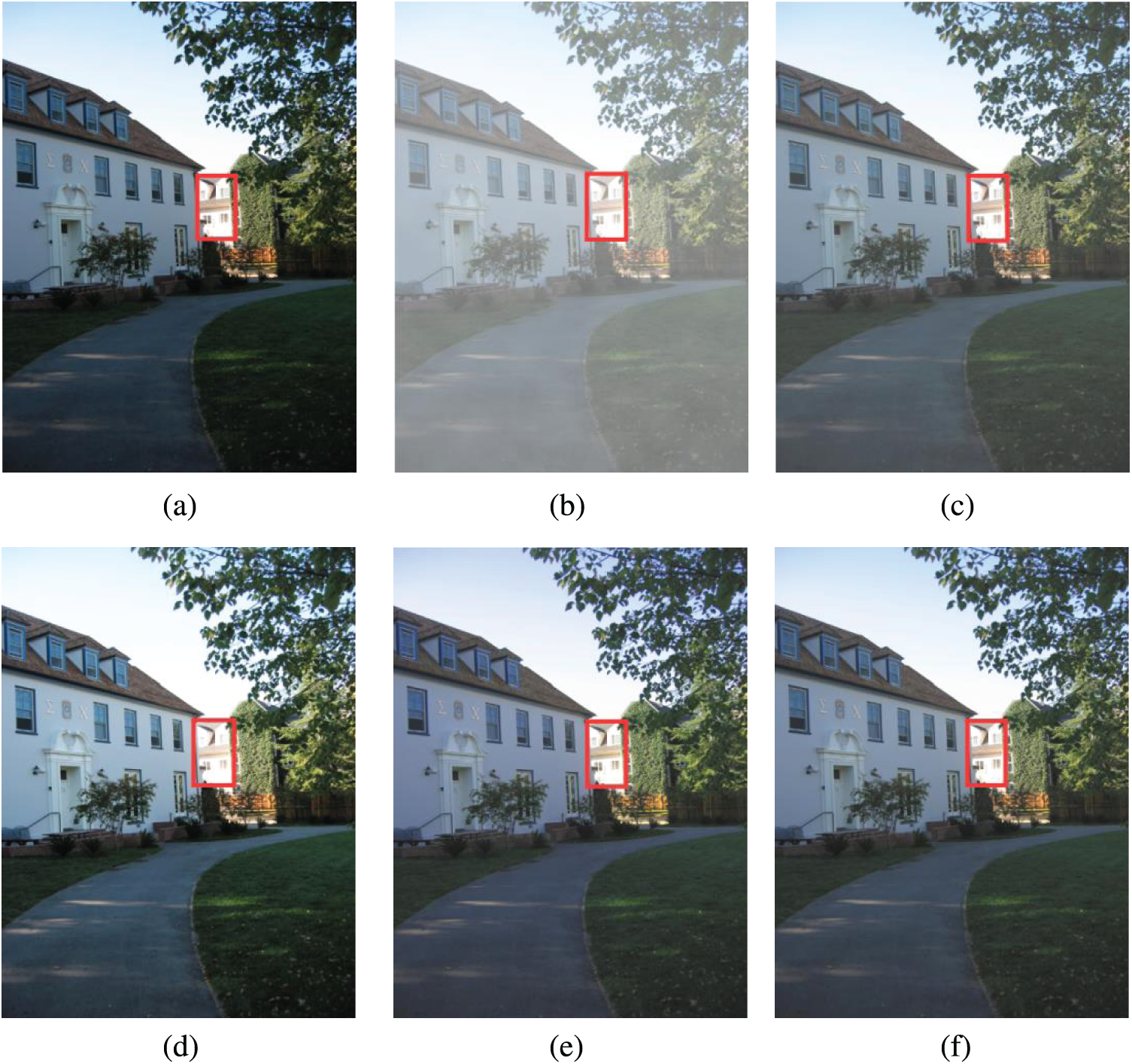
Figure 6: Comparison results of the dehazing of the house images. (a) Sharp image. (b) Synthetic hazy image. (c) Tang’s algorithm. (d) Cai’s algorithm. (e) Li’s algorithm. (f) Our approach
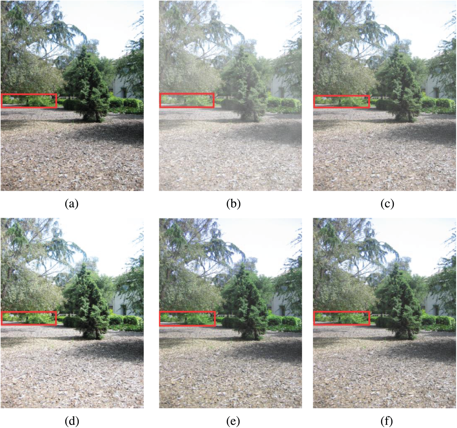
Figure 7: Comparison results of the dehazing of the tree images. (a) Sharp image. (b) Synthetic hazy image. (c) Tang’s algorithm. (d) Cai’s algorithm. (e) Li’s algorithm. (f) Our approach
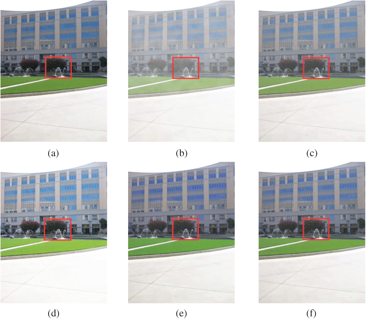
Figure 8: Comparison results of the dehazing of the fountain images. (a) Sharp image. (b) Synthetic hazy image. (c) Tang’s algorithm. (d) Cai’s algorithm. (e) Li’s algorithm. (f) Our approach
(2) Results of Real Hazy Image
To verify the effect of the FT-DCRN dehazing algorithm on real hazy images, we analyze 1200 real hazy images of outdoor scenes, such as building, garden and parking area. We compare the results of the FT-DCRN with those of Tang’s algorithm, Cai’s algorithm and Li’s algorithm. Fig. 9 show the comparison results of the dehazing of the images of building.

Figure 9: Comparison results of the dehazing of the building images. (a) Sharp image. (b) Real hazy image. (c) Tang’s algorithm. (d) Cai’s algorithm. (e) Li’s algorithm. (f) Our approach
Fig. 9 show that Tang’s algorithm results in unclear boundaries for the buildings. Cai’s algorithm easily produces color distortion, which makes the scene of the buildings look unreal. Li’s algorithm changes the color of the white areas. Our approach has clear boundaries and textures, and the overall colors of the images are close to the normal visual effect.
To perform the quantitative evaluation, synthetic hazy images and real hazy images are selected. We adopt the structural similarity (SSIM) [32], peak signal-to-noise ratio (PSNR) [33] and information entropy (IE) [34] to evaluate the effect of the FT-DCRN dehazing algorithm. The SSIM is an indicator of the similarity of two images. When two images are the same, the SSIM is equal to 1. The PSNR is a statistical indicator that is based on the gray values of image pixels. The higher the PSNR is, the better the image restoration. The IE is a statistical measure of features that reflects the average amount of information in the image. The larger the entropy is, the clearer the image. The experimental results for the synthetic hazy image are shown in Tabs. 1–4.
Table 1: Experimental results for the synthetic hazy road images
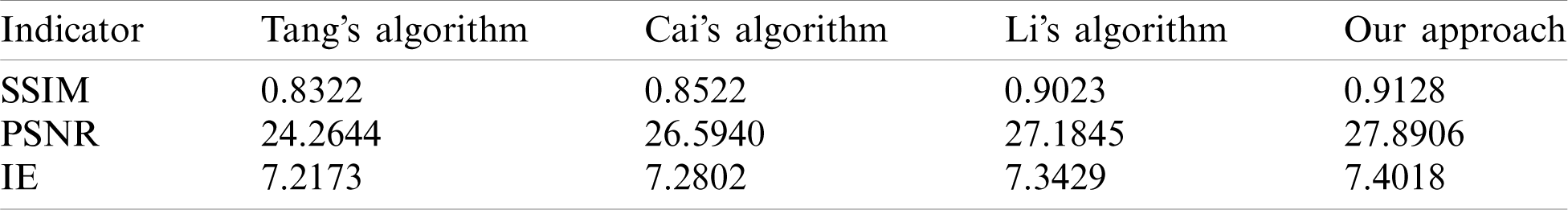
Table 2: Experimental results for the synthetic hazy house images
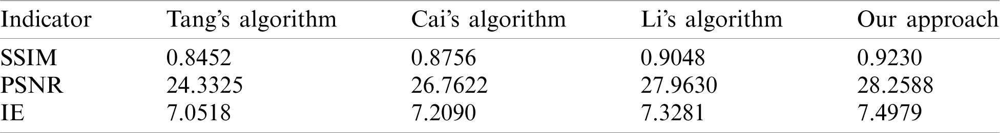
Table 3: Experimental results for the synthetic hazy tree images
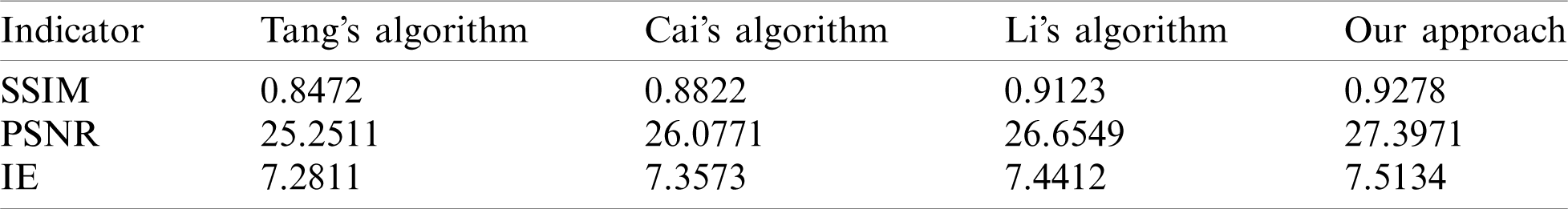
Table 4: Experimental results for the synthetic hazy fountain images
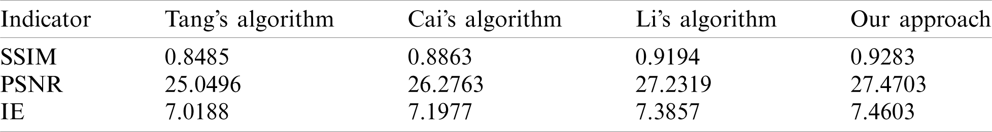
The results of Tang’s algorithm provided relatively low values for each indicator. Tang’s algorithm did not use the texture features in the image, which creates certain limitations on the dehazing effect. Cai’s algorithm and Li’s algorithm have significantly higher SSIM and PSNR values than those of Tang’s algorithm. However, Cai’s algorithm and Li’s algorithm do not result in normal visual color effects in Figs. 5–8. The IE of our approach is higher than those of other algorithms, which reflects that the dehazed image retains more detail and texture information.
3.3 Experiment of ARI-SFM Algorithm
3.3.1 Results of 3D Reconstruction
Figs. 10a–10f includes six images of a building taken from different perspectives. The images of the building from different perspectives are taken from a real scene.
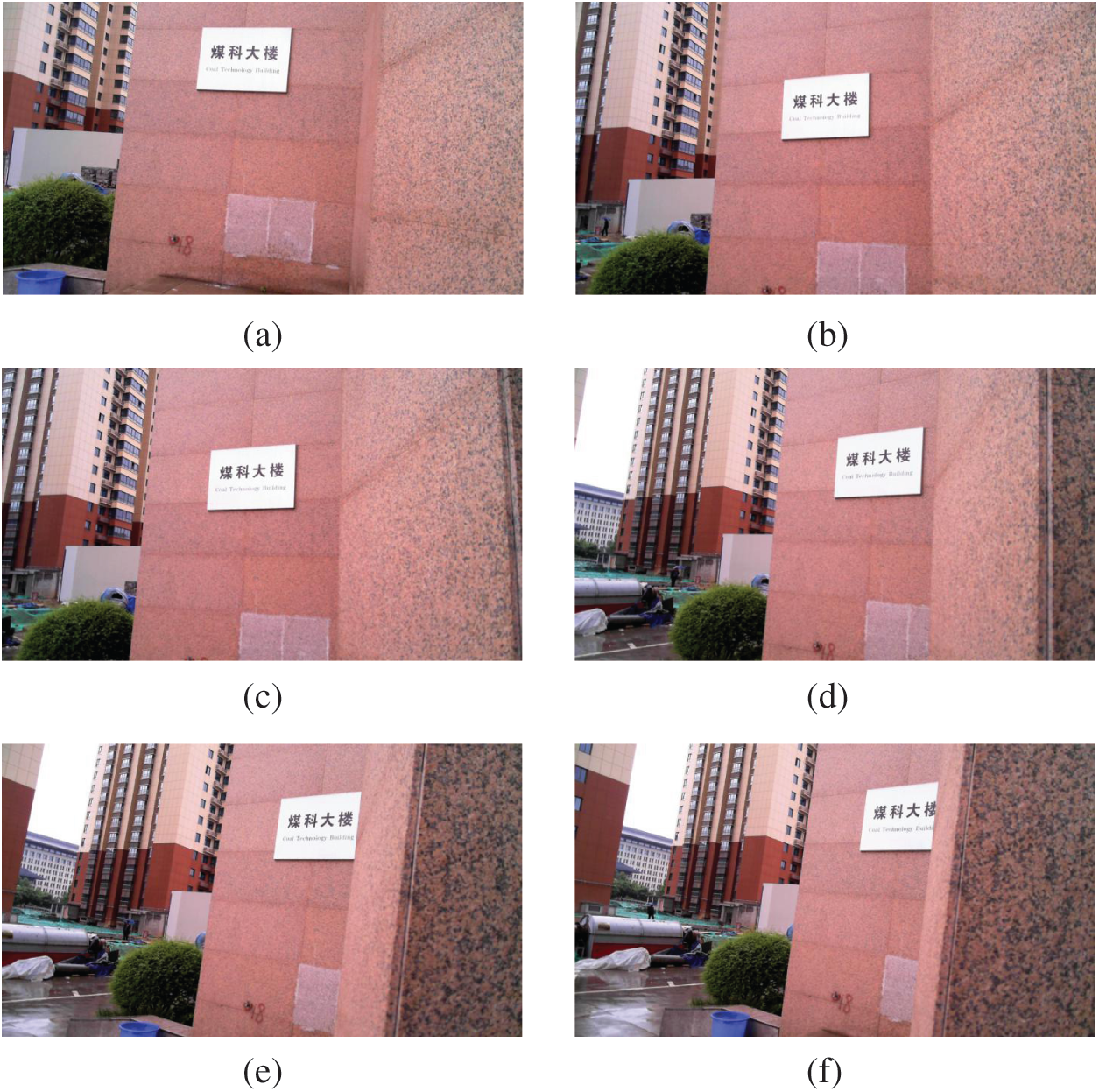
Figure 10: Six images of a building taken from different perspectives. (a) First perspective. (b) Second perspective. (c) Third perspective. (d) Fourth perspective. (e) Fifth perspective. (f) Sixth perspective
After using the ARI-SFM algorithm, the one-to-one relationship between corners is determined, and one-to-many relationship almost does not exist. In this experiment, we selected 6 images shown in Fig. 10 for 3D reconstruction. The final experimental results are shown in Fig. 11. Fig. 11 is the point cloud of 3D reconstruction of building. The Fig. 11 shows that the ARI-SFM algorithm can accurately reconstruct the 3D building, and the signs on the building are clearly visible.
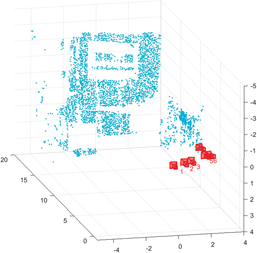
Figure 11: Point cloud of 3D reconstruction of building
3.3.2 Performance of 3D Reconstruction
To verify the matching efficiency of the ARI-SFM algorithm, the results of the algorithm are compared with some representative algorithms. Because different image matching algorithms have their own advantages, we adopt the Hossain’s algorithm [15], Zhang’s algorithm [16] and Zhou’s algorithm [17], which are described in the introduction. We analyze the comparison of the matching results of the building, as shown in Tab. 5.
Table 5: Comparison of the matching results of the building
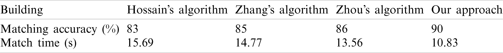
Tab. 5 show that our approach have higher matching accuracy and cost less match time, which indicates that we guarantee the precision and improve the efficiency compared with other algorithms. Our approach determine the one-to-one relationship between corners and almost does not exist one-to-many relationship, which obtains fine matching corner pairs and reduces the number of iterations.
AI solutions can provide great help for dehazing images, which can automatically identify patterns or monitor the environment. Therefore, we propose a 3D reconstruction method for dehazed images for smart cities based on deep learning. First, we propose an FT-DCRN dehazing algorithm that uses fine transmission images and atmospheric light values to compute dehazed images. The DCRN is used to obtain the coarse transmission image, which can not only expand the receptive field of the network, but can also retain the features to maintain the nonlinearity of the overall network. The fine transmission image is obtained by refining the coarse transmission image using a guided filter. The atmospheric light value is estimated according to the position and brightness of the pixels in the original hazy image. Second, we use the dehazed images generated by the FT-DCRN dehazing algorithm for 3D reconstruction. The ARI-SFM algorithm, which obtains the fine matching corner pairs and reduces the number of iterations, establishes an accurate one-to-one matching corner relationship. The experimental results show that our FT-DCRN dehazing algorithm improves the accuracy compared to other representative algorithms. In addition, the ARI-SFM algorithm guarantees the precision and improves the efficiency.
Developing AI systems supporting smart cities requires considerable data. Through the acquisition of effective information, smart cities can truly become sustainable developments. By 2021, one billion smart cameras will be deployed in infrastructure and commercial buildings. The large amount of raw data collected is far beyond the scope that can be viewed, processed or analyzed manually. Through the machine learning training process, images can be analyzed for city planning and development. AI algorithms have become the developmental trend and key point of smart cities [35]; therefore, how to manage deep learning algorithms, data, software, hardware and services will become another problem in the future.
Acknowledgement: The author would like to thank the anonymous reviewers for their valuable comments and suggestions that improve the presentation of this paper.
Funding Statement: This work was supported in part by the National Natural Science Foundation of China under Grant 61902311 and in part by the Japan Society for the Promotion of Science (JSPS) Grants-in-Aid for Scientific Research (KAKENHI) under Grant JP18K18044.
Conflicts of Interest: The authors declare that they have no conflicts of interest to report regarding the present study.
1. Z. Guo, K. Yu, Y. Li, G. Srivastava and J. C.-W. Lin, “Deep learning-embedded social internet of things for ambiguity-aware social recommendations,” IEEE Transactions on Network Science and Engineering, pp. 1, 2021. https://doi.org/10.1109/TNSE.2021.3049262. [Google Scholar]
2. K. Yu, L. Lin, M. Alazab, L. Tan and B. Gu, “Deep learning-based traffic safety solution for a mixture of autonomous and manual vehicles in a 5G-enabled intelligent transportation system,” IEEE Transactions on Intelligent Transportation Systems, pp. 1–11, 2020. https://doi.org/10.1109/TITS.2020.3042504. [Google Scholar]
3. L. Zhao, K. Yang, Z. Tan, X. Li, S. Sharma et al., “A novel cost optimization strategy for SDN-enabled UAV-assisted vehicular computation offloading,” IEEE Transactions on Intelligent Transportation Systems, pp. 1–11, 2020. https://doi.org/10.1109/TITS.2020.3024186. [Google Scholar]
4. M. Y. Ju, Z. F. Gu and D. Y. Zhang, “Single image haze removal based on the improved atmospheric scattering model,” Neurocomputing, vol. 260, no. 18, pp. 180–191, 2017. [Google Scholar]
5. K. T. Tang, J. C. Yang and J. Wang, “Investigating haze-relevant features in a learning framework for image dehazing,” in Proc. of IEEE Conf. on Computer Vision and Pattern Recognition, Columbus, IEEE, pp. 2995–3002, 2014. [Google Scholar]
6. B. Cai, X. M. Xu, K. Jia, C. Qing and D. C. Tao, “DehazeNet: An end-to-end system for single image haze removal,” IEEE Transactions on Image Processing, vol. 25, no. 11, pp. 5187–5198, 2016. [Google Scholar]
7. B. Y. Li, X. L. Peng, Z. Y. Wang, J. Z. Xu, D. Feng et al., “AOD-Net: All-in-one dehazing network,” in Int. Conf. on Computer Vision, Venice, IEEE, pp. 4770–4778, 2017. [Google Scholar]
8. Q. B. Wu, J. G. Zhang, W. Q. Ren and W. M. Zuo, “Accurate transmission estimation for removing haze and noise from a single image,” IEEE Transactions on Image Processing, vol. 29, pp. 2583–2597, 2020. [Google Scholar]
9. D. Park, D. K. Han and H. Ko, “Nighttime image dehazing using local atmospheric selection rule and weighted entropy for visible-light systems,” Optical Engineering, vol. 56, no. 5, pp. 050501, 2017. [Google Scholar]
10. M. Demant, P. Virtue, A. Kovvali, S. X. Yu and S. Rein, “Learning quality rating of as-cut mc-si wafers via convolutional regression networks,” IEEE Journal of Photovoltaics, vol. 9, no. 4, pp. 1064–1072, 2019. [Google Scholar]
11. Z. B. Wang, S. Wang and Y. Zhu, “Multi-focus image fusion based on the improved PCNN and guided filter,” Neural Processing Letters, vol. 45, no. 1, pp. 75–94, 2017. [Google Scholar]
12. G. L. Bi, J. Y. Ren, T. J. Fu, T. Nie, C. Z. Chen et al., “Image dehazing based on accurate estimation of transmission in the atmospheric scattering model,” IEEE Photonics Journal, vol. 9, no. 4, pp. 7802918, 2017. [Google Scholar]
13. J. Zhang, K. P. Yu, Z. Wen and X. Qin, “3D reconstruction for motion blurred images using deep learning-based intelligent systems,” Computers, Materials & Continua, vol. 66, no. 2, pp. 2087–2104, 2021. [Google Scholar]
14. E. Casella, A. Collin, D. Harris, S. Ferse, S. Bejarano et al., “Mapping coral reefs using consumer-grade drones and structure from motion photogrammetry techniques,” Coral Reefs, vol. 36, no. 1, pp. 269–275, 2017. [Google Scholar]
15. M. A. Hossain and A. K. Tushar, “Chord angle deviation using tangent (CADTan efficient and robust contour-based corner detector,” in Proc. of IEEE Int. Conf. on Imaging, Vision & Pattern Recognition, Dhaka, Bangladesh, IEEE, pp. 1–6, 2017. [Google Scholar]
16. H. L. Zhang, Z. Gao, X. J. Zhang and K. F. Shi, “Image matching method combining hybrid simulated annealing and antlion optimizer,” Computer Science, vol. 46, no. 6, pp. 328–333, 2019. [Google Scholar]
17. W. Zhou, A. N. Bowen, M. Zhao and S. Pan, “Heterologous remote sensing image registration algorithm based on geometric invariance and local similarity features,” Infrared Technology, vol. 41, no. 6, pp. 561–571, 2019. [Google Scholar]
18. C. H. Yeh, C. H. Huang and L. W. Kang, “Multi-scale deep residual learning-based single image haze removal via image decomposition,” IEEE Transactions on Image Processing, vol. 29, pp. 3153–3167, 2019. [Google Scholar]
19. S. C. Raikwar and S. Tapaswi, “Lower bound on transmission using non-linear bounding function in single image dehazing,” IEEE Transactions on Image Processing, vol. 29, pp. 4832–4847, 2020. [Google Scholar]
20. H. Zhu, R. Vial and S. Lu, “TORNADO: A spatio-temporal convolutional regression network for video action proposal,” in 2017 IEEE Int. Conf. on Computer Vision, Venice, IEEE, pp. 5814–5822, 2017. [Google Scholar]
21. L. Zhao, Y. Liu, A. Al-Dubai, Z. Tan, G. Min et al., “A novel generation adversarial network-based vehicle trajectory prediction method for intelligent vehicular networks,” IEEE Internet of Things Journal, vol. 8, no. 3, pp. 2066–2077, 2020. [Google Scholar]
22. L. Qin, Y. Gong, T. Tang, Y. Wang and J. Jin, “Training deep nets with progressive batch normalization on multi-GPUs,” International Journal of Parallel Programming, vol. 47, no. 3, pp. 373–387, 2019. [Google Scholar]
23. H. Y. Jung and Y. S. Heo, “Fingerprint liveness map construction using convolutional neural network,” Electronics Letters, vol. 54, no. 9, pp. 564–566, 2018. [Google Scholar]
24. Y. F. He, A. Carass, Y. H. Liu, B. M. Jedynak, S. D. Solomon et al., “Structured layer surface segmentation for retina OCT using fully convolutional regression networks,” Medical Image Analysis, vol. 68, no. 136295, pp. 101856, 2020. [Google Scholar]
25. L. Liu, C. Shen and A. V. D. Hengel, “Cross-convolutional-layer pooling for image recognition,” IEEE Transactions on Pattern Analysis & Machine Intelligence, vol. 39, no. 11, pp. 2305–2313, 2015. [Google Scholar]
26. J. Yuan, H. C. Xiong, Y. Xiao, W. L. Guan, M. Wang et al., “Gated CNN: Integrating multi-scale feature layers for object detection,” Pattern Recognition, vol. 105, no. 6, pp. 107131, 2019. [Google Scholar]
27. R. Xiang, X. Zhu, F. Wu and X. Y. Jiang, “Guided filter based on multikernel fusion,” Journal of Electronic Imaging, vol. 26, no. 3, pp. 033027.1–033027.8, 2017. [Google Scholar]
28. K. He, J. Sun and X. Tang, “Single image haze removal using dark channel prior,” in Proc. of IEEE Conf. on Computer Vision and Pattern Recognition, Miami, IEEE, pp. 1956–1963, 2009. [Google Scholar]
29. S. Q. Dong, L. G. Han, Y. Hu and Y. C. Yin, “Full waveform inversion based on a local traveltime correction and zero-mean cross-correlation-based misfit function,” Acta Geophysica, vol. 68, no. 1, pp. 29–50, 2020. [Google Scholar]
30. L. Piermattei, L. Carturan, F. DBlasi and P. Tarolli, “Suitability of ground-based SFM-MVS for monitoring glacial and periglacial processes,” Earth Surface Dynamics, vol. 4, no. 2, pp. 425–443, 2016. [Google Scholar]
31. L. Bo, D. Yuchao and H. Mingyi, “Monocular depth estimation with hierarchical fusion of dilated CNNs and soft-weighted-sum inference,” Pattern Recognition, vol. 83, pp. 328–339, 2017. [Google Scholar]
32. T. S. Zhao, J. H. Wang, Z. Wang and C. W. Chen, “SSIM-based coarse-grain scalable video coding,” IEEE Transactions on Broadcasting, vol. 61, no. 2, pp. 210–221, 2015. [Google Scholar]
33. M. Malarvel, G. Sethumadhavan, P. C. R. Bhagi, S. Kar, T. Saravanan et al., “Anisotropic diffusion based denoising on X-radiography images to detect weld defects,” Digital Signal Processing, vol. 68, pp. 112–126, 2017. [Google Scholar]
34. X. Zhang, D. Li, J. Li and Y. Li, “Magnetotelluric signal-noise separation using IE-LZC and MP,” Entropy, vol. 21, no. 12, pp. 1190–1204, 2019. [Google Scholar]
35. Z. Guo, K. Yu, A. Jolfaei, A. K. Bashir, A. O. Almagrabi et al., “A fuzzy detection system for rumors through explainable adaptive learning,” IEEE Transactions on Fuzzy Systems, pp. 1, 2021. https://doi.org/10.1109/TFUZZ.2021.3052109. [Google Scholar]
 | This work is licensed under a Creative Commons Attribution 4.0 International License, which permits unrestricted use, distribution, and reproduction in any medium, provided the original work is properly cited. |