DOI:10.32604/cmc.2021.014768
| Computers, Materials & Continua DOI:10.32604/cmc.2021.014768 | |
| Article |
Stock Price Prediction Using Predictive Error Compensation Wavelet Neural Networks
1Graduate School of Science Engineering and Technology, Istanbul Technical University, Istanbul, Turkey
2Department of Computer Engineering, Istanbul Technical University, Istanbul, Turkey
*Corresponding Author: Ajla Kulaglic. Email: kulaglic@itu.edu.tr
Received: 14 October 2020; Accepted: 09 March 2021
Abstract: Machine Learning (ML) algorithms have been widely used for financial time series prediction and trading through bots. In this work, we propose a Predictive Error Compensated Wavelet Neural Network (PEC-WNN) ML model that improves the prediction of next day closing prices. In the proposed model we use multiple neural networks where the first one uses the closing stock prices from multiple-scale time-domain inputs. An additional network is used for error estimation to compensate and reduce the prediction error of the main network instead of using recurrence. The performance of the proposed model is evaluated using six different stock data samples in the New York stock exchange. The results have demonstrated significant improvement in forecasting accuracy in all cases when the second network is used in accordance with the first one by adding the outputs. The RMSE error is 33% improved when the proposed PEC-WNN model is used compared to the Long Short-Term Memory (LSTM) model. Furthermore, through the analysis of training mechanisms, we found that using the updated training the performance of the proposed model is improved. The contribution of this study is the applicability of simultaneously different time frames as inputs. Cascading the predictive error compensation not only reduces the error rate but also helps in avoiding overfitting problems.
Keywords: Predictive error compensating wavelet neural network; time series prediction; stock price prediction; neural networks; wavelet transform
The stock markets are 80% controlled by machines and over the next 10 years, robots will replace 200,000 banking jobs according to an article published in Forbes [1]. The high-frequency trading technologies represent a type of algorithmic trading that uses machine learning algorithms to implement investment strategies in extremely small-time intervals. Algorithmic trading has a major effect on the way financial assets change hands [2]. Chague et al. [3] found that 97% of day traders end up losing money as a year approach. Similar studies found that only 1% of traders make money and have some level of profitability after costs [4,5]. Despite the evidence of negative consequences discussed in [1], the full effects of algorithm trading are yet to be seen. In the stock market, the stock price prediction mechanisms are fundamental to the formation of investment strategies and the development of risk management models [6]. As the stock market influences individual and national economies, the prediction of the stock market is an essential task while taking the proper decision [7]. However, due to the uncertainty in financial time series data, the accurate prediction of stock market changes represents a challenging task. For this reason, in the proposed study by evaluating input data in multiple networks we tried to forecast the next day closing stock price. The networks are used in an additive manner. The first network is used as the main predictor. An additional network is used for the prediction of the main network error to compensate the overall daily stock prediction error. The prediction performance is significantly improved using the proposed model by reducing the overfitting and without increasing the complexity of the proposed algorithm.
Early researches on stock market prediction were based on random walk theory and Efficient Market Hypothesis (EMH) [8]. The EMH states that current stock prices reflect all the available information, and show that it is not possible to predict future stock prices using past information. Furthermore, Malkiel et al. [8] argued that any new information is immediately reflected in price changes without delay, and therefore future asset price movements are independent of past and current information. The suggestions made in [8] are that stock prices cannot be predicted since they are driven by external and new information rather than just historical or current prices. Moreover, the stock price data are disposed to frequent changes that cannot be derived from a historical trend. On the other hand, numerous studies have attempted to experimentally disprove the study of Malkiel et al. [8] by showing that stock markets are predictable. Bachelier [9] first proposed the efficient market theory and described the stock price movement in the random walk manner. Later, the random walk characteristics of changes in prices were empirically tested by Cootner [10] and Fama [11]. The changes are influenced by real-world factors, such as political, social, and environmental factors [12]. In addition, the noise to signal ratio is very high in such conditions and it is difficult to analyze and forecast future data. The use of econometric models is convenient for describing and evaluating the relationships between variables using statistical inference, with some limitations. These limitations can be seen in not being able to capture the nonlinear nature of stock prices. In addition [13], in their study assumed to have constant variance while the financial time series is very noisy and has time-varying volatility. Thus, by the work done in the [14], it is concluded that the stock market price will follow a random walk and prediction accuracy cannot exceed 50%.
The statistical methods, such as Autoregressive Moving Average (ARMA), Autoregressive Integrated Moving Average (ARIMA), and vector autoregression have generally achieved reasonable predicting results based on the literature results [15–20]. These statistical models map linear relationships but they are not very useful in stock market prediction due to the nature of stock market data. ARIMA is one of the most popular and widely used statistical techniques for making predictions using past observations [17]. In the work of Nochai et al. [18], they intend to find an appropriate ARIMA model. The empirical analysis of the study showed that ARIMA (2, 1, 0), (1, 0, 1), and (3, 0, 0) are the best models for predicting the price of palm oil. Viswanatha Reddy [19] in his work tries to check the stationarity in time series data and predict the direction of change in the stock market index using the ARIMA model. The best results are obtained for ARIMA (0, 1, 0). The author in his study confirmed the perspective of the ARIMA model to forecast future time series in a short time.The study of Adebiyi et al. [20] is conducted for predicting the share prices during the short-run. The results of this study showed that ARIMA models have power in predicting stock prices in a short time.
Despite the above mentioned statistical models, Artificial Neural Networks (ANNs) are one of the most accurate prediction models [21]. According to [22], the ANNs, unlike statistical models, with given sufficient amounts of data can approximate any finite and continuous function based on the universal approximation theorem. A forecasting system based on radial basis function Neural Network (NN) proposed by Lendasse et al. [23] showed that the system can capture the nonlinear relationship in financial time series data. The first significant study of neural network models for stock price return prediction was accomplished by White [2] where he introduces the predictive model based on IBM’s daily common stock and achieved promising results. In order to increase the prediction performance, hybrid models have shown significant achievements. Different hybrid systems were proposed by using ANNs, the Hidden Markov Model (HMM) [24], exponential smoothing, and ARIMA [25]; and ANN with exponential generalized autoregressive conditional heteroscedasticity model [26]. Yao et al. [27] compared the back-propagation NN model with the ARIMA model. They found that the NN results in better prediction accuracy, comparing to the ARIMA models. Adebiyi et al. [28] compared the performances of the ARIMA and ANN models for stock price prediction and found the superiority of the NN model over the ARIMA model. On the other hand, Nitin et al. [29] did a comparative study of a three-layer feed-forward NN model and the ARIMA model to predict future stock price data and revealed that the ARIMA models perform better over NN models. Similar to [29], Lee et al. [30] developed the NN model and the Seasonal Autoregressive Integrated Moving Average (SARIMA) model for stock index prediction. In their results, they also found that the ARIMA model outperforms ANN models for stock prediction. The results show that the model results depend on the data. Furthermore, using ARIMA together with ANN, as a new hybrid model improves the prediction performances. In this work, the empirical results reveal that hybrid systems outperform all individual systems providing more accurate prediction performances.
The two most popular deep-learning architectures for stock market forecasting in recent years are the Long Short-Term Memory (LSTM) model and the Gated Recurrent Unit (GRU) model with its hybridization [31]. The LSTM models are appropriately structured to learn temporal patterns and overperform the conventional recurrent neural networks (RNNs) as it overcomes the problem of vanishing gradients. Shahi et al. [31] proposed the LSTM and GRU deep-learning architectures and compare the performances of these two models for stock market prediction. In their study, they made a comparison on the performances of the LSTM and GRU models under the same conditions and also showed that by including the financial news sentiments together with the stock market features the predicting model can be significantly improved. Bao et al. [32] used the LSTM for stock price forecasting using different types of sequential data. Li et al. [33] using the sentiment features showed that LSTMs outperform benchmark models of SVM and improve the accuracy of prediction of the next day’s open price.
The problem of overfitting and getting stuck in local optima are additional issues that have to be taken into consideration in prediction models. The problem occurs due to data amount limitations and appropriate model configuration. The NN models even though achieve better generalization, are prone to overfitting due to their high capacity. In the financial time series forecasting using the Deep Neural Networks (DNNs), overfitting occurs due to a lack of data [34]. The financial time series data in a year on a daily basis obtain approximately 252 data points. However, it is insufficient for the DNN models in comparison to the number of model parameters. Sufficient data is needed as the number of model parameters increases as we enlarge the number of features used. Considering that overfitting impairs prediction accuracy regularization techniques, such as dropout, early stopping, data augmentation, or reducing the network size and learning rate are needed to avoid this problem [35]. The regularization techniques can prevent overfitting, but it cannot improve generalization performance. Hence, data augmentation is a method used to prevent overfitting while improving generalization accuracy. However, when it is about the financial time series, the data augmentation distorts the original data which is not a simple task. Instead, in recent times, signal processing techniques have been used to transform the data into a format that reveals certain characteristics. The results showed that using the extracted features can achieve more accurate predictions than using the data without feature extraction. The Fourier Transformation (FT) enables a signal to be expressed with a certain characteristic, however, a severe disadvantage is that the time resolution is missing. In addition, Wavelet Transform (WT) is proposed to overcome this disadvantage and the time series mostly uses different variations of the WT. Good local representation of a signal in both the time and frequency domain simultaneously is one of the main advantages of WT.
In this study, we propose the Wavelet Neural Network Model (WNN) for stock price time series data using a Predictive Error Compensation WNN (PEC-WNN) model. The research is conducted based on two separately trained NNs where input data are preprocessed using a Discrete Wavelet Transform (DWT). The motivation for using two separate NNs comes from the following perspectives. Firstly, the forecasting models are facing with expending uncertainties such as lack of input data for making more accurate predictions and secondly, a well-known drawback in the recursive methods, the accumulation of errors since the predicted values are used in the model instead of the target values. The proposed model is independently trained and not inclines the accumulated errors. The compensation of the predicted error through the second NN enhances the overall prediction performance.
This article does not propose trading strategies despite the evidence of asset price predictability presented here. We present and evaluate the prediction performance of our model based on different companies in which data are publicly available using the Yahoo Finance website [36].
The remainder of this paper is organized as follows. Section 2 describes the proposed model. The dataset specification and construction are explained in Subsection 2.1. The proposed method’s model description and characteristics are given in Subsection 2.2. The experimental results with discussion are given in Section 3. Conclusion and suggested future work remarks are given in Section 4.
2 Predictive Error Compensation Wavelet Neural Network Model
When machine learning methods are used for time series prediction of stochastic data sets, their time series error patterns usually include residual information. These error patterns may depend on the inconsistency of sampling time interval, scale, inappropriate machine learning structure, overfitting, underfitting, or time-varying characteristics of the data resource. A conventional way of reducing the prediction error is using past prediction errors through additional inputs or recurrences in NNs [32]. This also increases the requirement of larger training data sets and training more amount of weights to avoid overfitting and better characterization of the input data patterns. Instead of applying the error data patterns back into the same network through the increased amount of inputs and nodes, we propose using an additional NN that is trained by the error of the first NN. Specifically, when the WT of the input data patterns and the error data patterns are used in this method (PEC-WNN) overall accuracy significantly raises while the time complexity remains less than the unified network equivalent of the solution [37]. This proposed data efficiency raising strategy can then be extended by using more amount of NNs trained by the error pattern of the superposed prediction and additional data can also be fused. The PEC-WNN model is shown in Fig. 1.
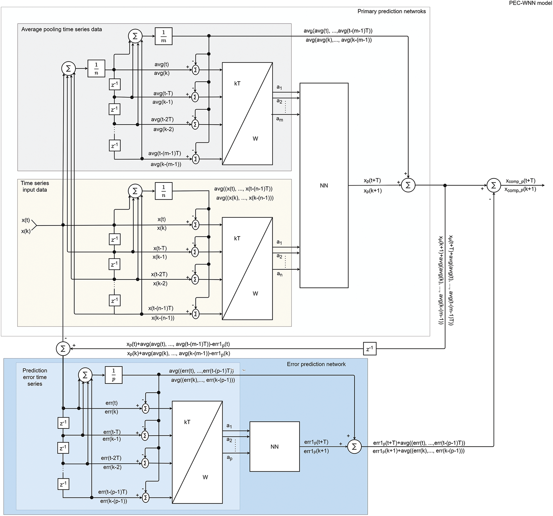
Figure 1: Predictive error compensation wavelet neural network (PEC-WNN) model for stock price forecasting
In this section, we explain the proposed PEC-WNN structure and demonstrate its performance on the prediction of the next day closing price in the stock exchange. A key factor in this improvement is the schematic of training the networks as shown in Fig. 2. The main network, in the figure, represented as WNN 1 uses the closing stock price data through moving frames in single and multiple-time scales as inputs for closing price predictions. In Fig. 2, the eight consecutive values in a single time scale are represented. An additional network, in the figure presented as WNN 2, uses the error patterns computed with the predictions of the main network (WNN 1). Finally, the predictive closing price from the WNN 1 and the predictive error from WNN 2 are used together to acquire the compensated predictive closing stock price.
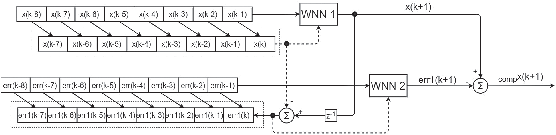
Figure 2: The schematic representation of training the networks
The proposed networks are characterized by three-layer NN architecture. The optimal number of neurons in the hidden layers is obtained based on the trial and error method considering the formulas proposed in the literature [38–40]. The formula proposed by Patterson (Eq. (1)) in [40] is used since it generates the lowest prediction error.
where q is the number of hidden neurons, m and p are the numbers of inputs and output respectively, and N is the number of observations in the training dataset.
The employed networks use the Rectified Linear Unit (ReLU) activation function (Eq. (2)) that significantly improves the performance of the network compared to the widely used activation functions (sigmoid and hyperbolic tanged) [34].
The Stochastic Gradient Descent (SGD) algorithm is used as an optimization algorithm for both networks. The SGD maintains a single learning rate for all weight updates without varying during the training. The learning rate is maintained for each network weight, whereas it is distinctly adopted as learning folds. The learning rate and momentum are 0.05 and 0.75, respectively. In the Feed Forward Back-Propagation (FF-BP) model the “generalized delta rule” is used to update the weight for each unit as follows (Eq. (3)):
where the w(t) is the weight at time t,
The properties of the NNs used in this study are shown in Tab. 1.
In this work, we also investigated how learning of network affects the results besides different dataset construction strategies for the proposed method. In traditional learning, fixed training separates the input dataset into fixed training and test datasets [6]. Arnerić et al. [41] examine different ratios of separating input datasets to training and test samples (90/10, 80/20, 70/30, 60/40, and 50/50) and conclude that the lowest error is achieved using a 70/30 ratio. In this study for fixed training, we also divide the dataset using a 70/30 ration (the first 70% of data is used for training and the next 30% to test the model).
Continual training on the other side updates the training dataset after a certain amount of data has been tested and retrained the network again. In this experiment, the initial training is done by using the first 70% of the data. The initial test set is equally divided where the first 15% is used for initial testing. In the second stage, the training dataset is increased by 15% of the initial test data. Now, with 85% of the data, the previously constructed model is retrained and the test is done on the last 15% of the data. The scheme of the used learning algorithm is given in Fig. 3.
Table 1: The parameter settings of NN models
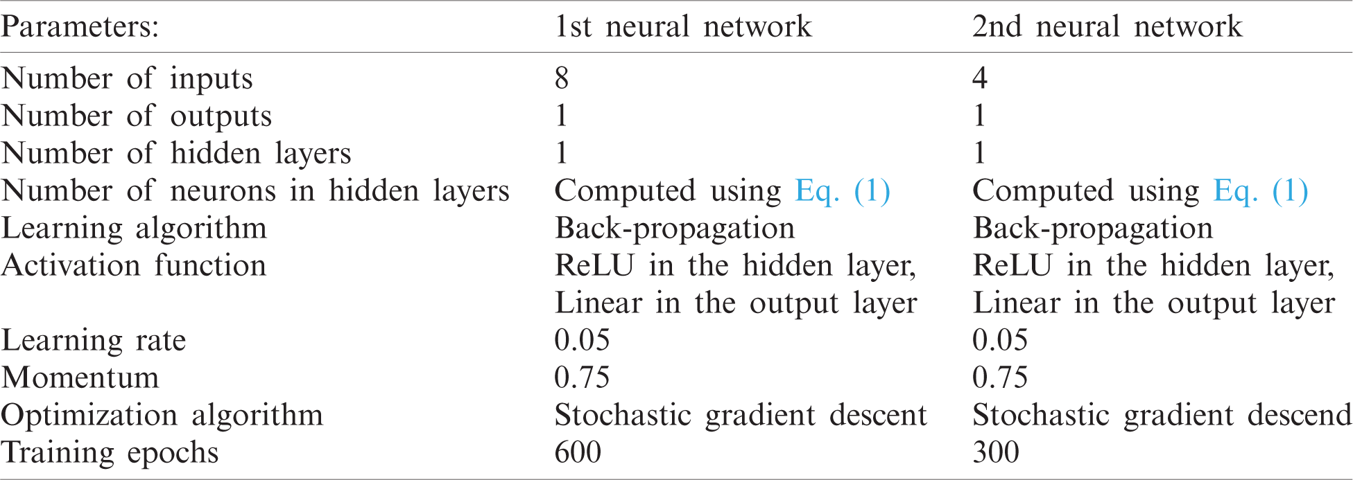
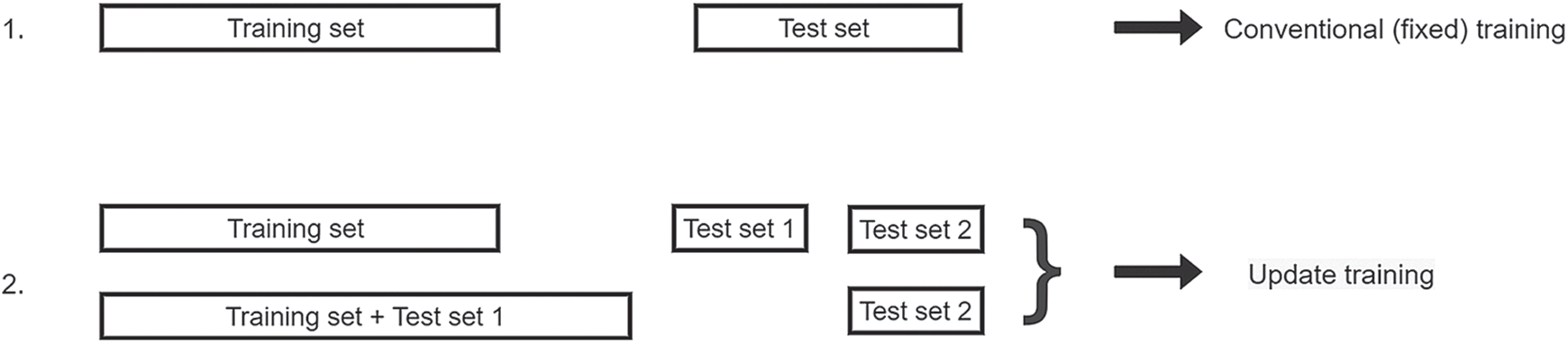
Figure 3: The conventional (fixed) and the updated training scheme
Historical stock price data for different companies are downloaded from Yahoo finance [36]. The page contains multiple stock markets of multiple companies with financial news, reports, and the facility to download historical data. The attributes of the downloaded dataset are given in Tab. 2. In this work for prediction of next day closing price, the daily closing prices are examined and used for the construction of datasets.
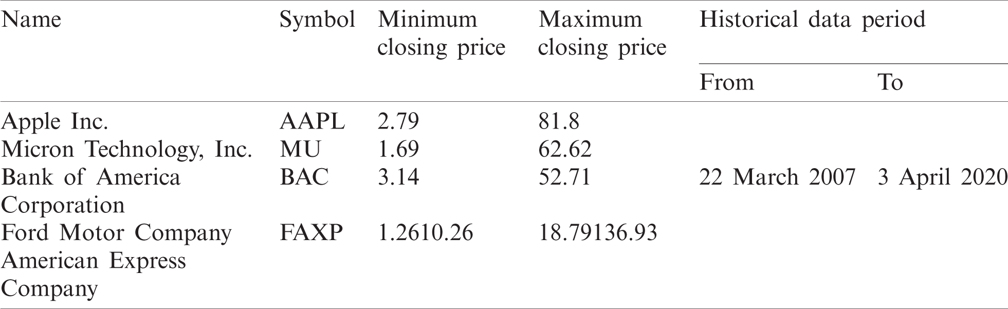
The stocks selected in this work are shown in Tab. 3. In this study, the daily prices of each of the stocks are collected from March 22, 2007 to April 3, 2020, what is a total of 13 years. The construction of datasets is done based on two strategies. The first is a single time window of consecutive values with different input sizes. The unit delay operator z−1 is used for the construction of the consecutive input dataset. The input size varies from four to eight business days. The second strategy involves the different time windows beside the consecutive values. At this stage, we include two different time frames where the average values of different time intervals are applied together with four consecutive values. In order to generate subsampled data, we applied separate averaging in time series data similar to the average pooling used in the Convolutional Neural Networks (CNNs). The time interval for calculating the average values is five. The calculations are organized in the same manner using the unit delay operator z−1. The reason for choosing five is to obtain the weekly resolution as in one week there are five closing prices. The four-weekly average values acquire the monthly resolution of input data.
Table 2: Attributes of the dataset
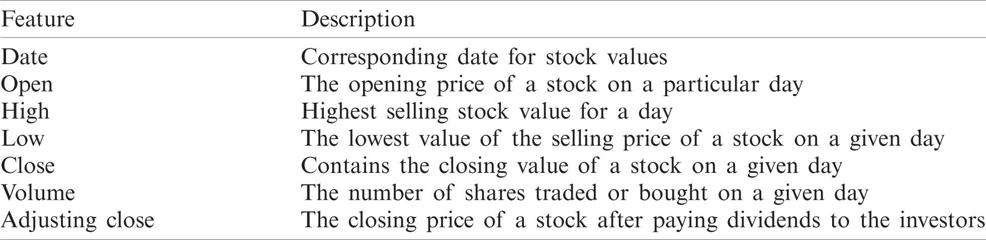
Table 3: The company information and period of the data used in this study
The constructed datasets from both strategies are normalized and preprocessed. Data normalization is a fundamental preprocessing step for mining and learning from the data [42]. Most of the traditional normalization methods make assumptions that the time series data are stationary and the volatility of the time series is uniform. However, these assumptions do not hold for most time series, especially not for the financial and economical time series. In the proposed algorithm, trying to avoid the problems caused by traditional normalization, we subtract the average value of all current inputs from the single value at the input. For the proposed strategy, where we have for example four days, we calculate the mean value of those four days and subtract the calculated average value from each day separately. The subtracted average value is added at the end of the forecasting process. The schematic representation of the proposed normalization is presented in Fig. 1. The preprocessing is done with a discrete wavelet transform (DWT) regarding the window frames. The aim of preprocessing is to extract features found within the time windows similar to the convolutional layers in CNNs. The gathered wavelet coefficients are used as inputs to the prediction model. The Haar wavelet basis function is utilized since it beneficially diminishes the distortion rate during the signal decomposition and reconstruction. Also, it significantly reduces processing and computational time.
Mallat’s pyramidal algorithm [43], of the second level that provides high (hn) and low (gn) frequencies from a given signal, is applied for decomposition. Both components are used together as inputs to the proposed model to capture valuable information during the training process. Fig. 4 shows a two-level wavelet decomposition structure of the input dataset that contains different window frames.
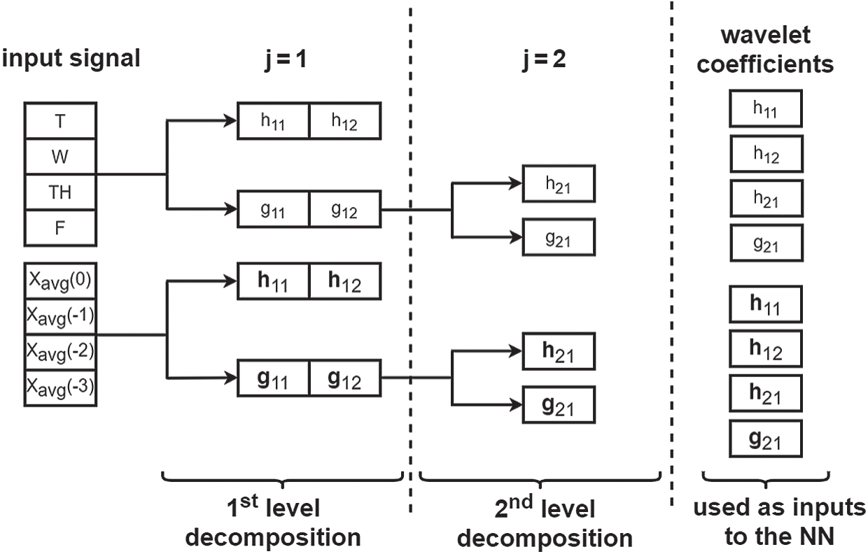
Figure 4: Multi-resolution wavelet decomposition. The block diagram of the wavelet decomposition using Mallat’s algorithm
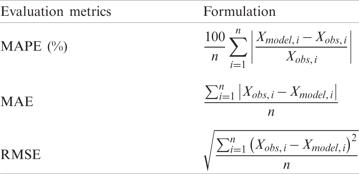
The forecasting performances of the proposed model are evaluated using the mean absolute percentage error (MAPE), the mean absolute error (MAE), and the root mean squared error (RMSE). The MAE considers the absolute deviation as the loss. It is more sensitive to small deviations and much less sensitive to large ones than the squared error. The MAE is also scale-dependent thus not suitable to compare prediction performance across different variables or ranges. An average measure of errors in the prediction of stock market indices represents the MAPE [44]. The average error is calculated without considering the directions of the set of predictions and each set of differences is having equal weight. The RMSE is a quadratic score principle used to determine the average magnitude of estimation error in stock market trends [44]. In addition, the RMSE depends on the scales and it is sensitive to outliers. The formulas are given in Tab. 4 where Xobs is observed and Xmodel is modeled values in time i. The number of data samples is given by n.
Table 4: The equations of used evaluation metrics
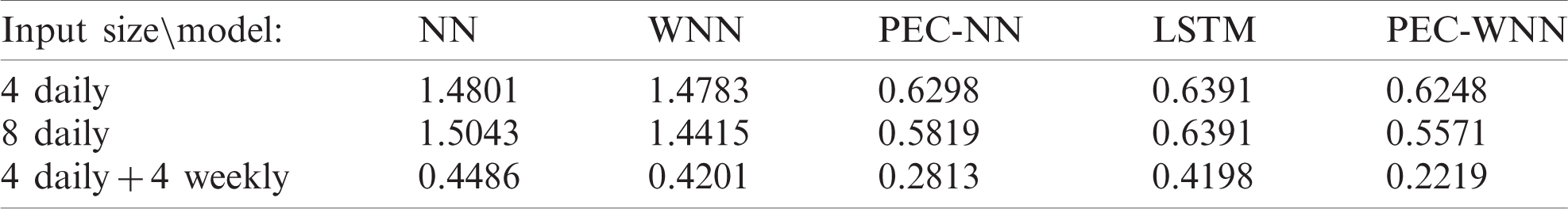
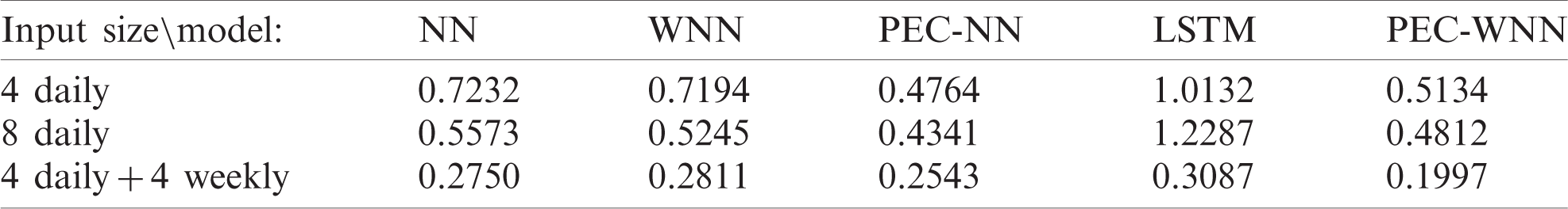
In the following parts, the obtained results are explained and discussed. The section considers the results of closing stock price predictions for six different companies. The results are analyzed concerning the proposed input data strategies, applied models, and by considering the training mechanism. The distinct input datasets are constructed concerning previously mentioned strategies and applied to five different models including the simple NN model (used below as NN), PEC-NN, WNN, LSTM, and PEC-WNN. The first dataset contains four, whereas the second dataset consists of eight consecutive values of closing stock prices. The third dataset consists of two distinct window frames, the four consecutive daily closing prices, and the four-weekly average values of current and previous three weeks. The four weekly average values of closing prices are used since it gives the monthly resolution of changes in the prices. The output of our model is the next day closing price. The network configuration of NN models is the same for each case. The main difference is in the preprocessing where the DWT is used. The LSTM model proposed by Roberts in [45] is used to compare the proposed model results with the model that is used in the field of deep learning. The LSTM model consists of one LSTM layer with 25 hidden units and a dense output. Moreover, the dropout regularization technique is applied to the hidden layer.
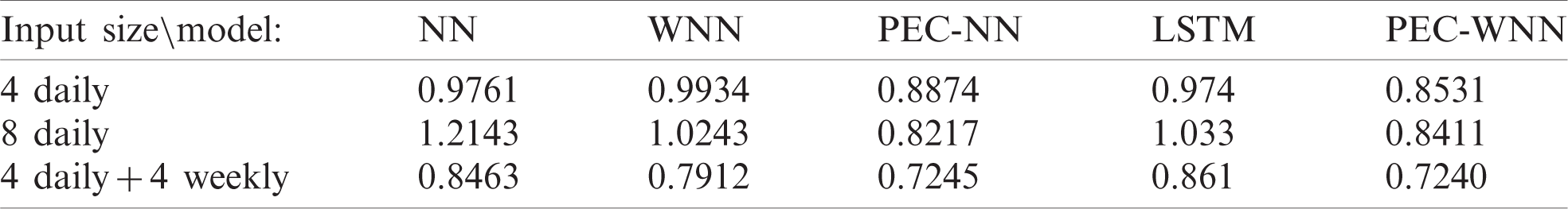
The results are analyzed concerning the proposed strategies, applied models, and by considering the training mechanism. Different companies and their closing prices were downloaded, arranged, and three different input datasets are constructed. The first dataset contains four, whereas the second dataset consists of eight consecutive values of closing stock prices. The third dataset consists of two different window frames, the four consecutive daily closing prices, and the four-weekly average values of current and three previous weeks. The four weekly average values of closing prices are used since it gives the monthly resolution of changes in the prices. The output of our model is the next day closing price. The prediction results for Ford (F) company are presented in Tabs. 5–7 for the training dataset and Tabs. 8–10 for the test dataset. The remaining results are presented as an average error with respect to the applied models in Fig. 5. The results have shown that the RMSE error is reduced when simultaneously different time frames are included with the proposed model. Increasing the number of inputs in a single window, from four to eight business days increase the RMSE error and does not show any improvements. On the other hand, with the usage of multiple time windows, the forecasting error is decreased. The proposed model PEC-WNN used together with the simultaneously different window frames achieves the lowest prediction error. The RMSE error for Ford stock price reduces by 42% comparing to the LSTM model when the predictive error compensation model is applied.
Table 5: The RMSE ($) training error results for the Ford company
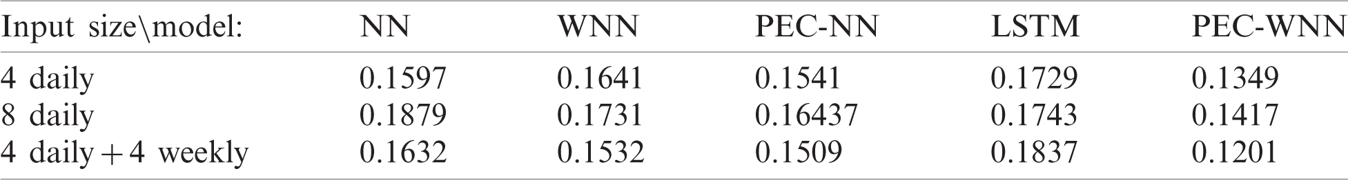
Table 6: The MAPE (%) training error results for the Ford company
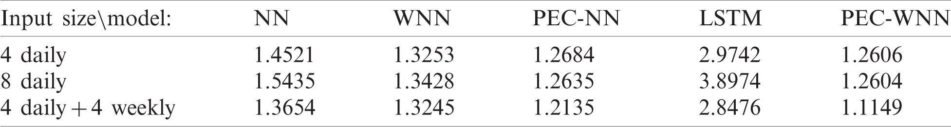
Table 7: The MAE ($) training error results for the Ford company
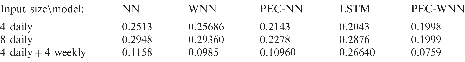
Table 8: The RMSE ($) test error results for the Ford company
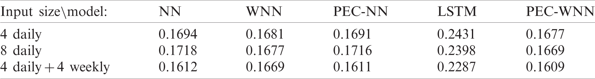
Table 9: The MAPE (%) test error results for the Ford company

Table 10: The MAE ($) test error results for the Ford company

The examination for update training is obtained regarding to the lowest error results reached with the best dataset. For that purpose, the second strategy is used, simultaneously different window frames with four consecutive values. In this part, the first 70% is used for initial training and the next 15% is applied as an initial test part. Later on, the updated training is performed by 85% of the dataset (70% from initial training +15% from the initial test) and the last 15% is used as a continual test part. The RMSE for the Ford closing prices is improved by 31.25% when the updated training mechanism is used.
The average RMSE, MAPE, and MAE results for the applied models are shown in Fig. 5. The average errors are computed for each model considering multiple time-framed datasets for six applied stock prices. From the graph, it can be seen that the proposed model achieves the lowest error comparing to the applied models.
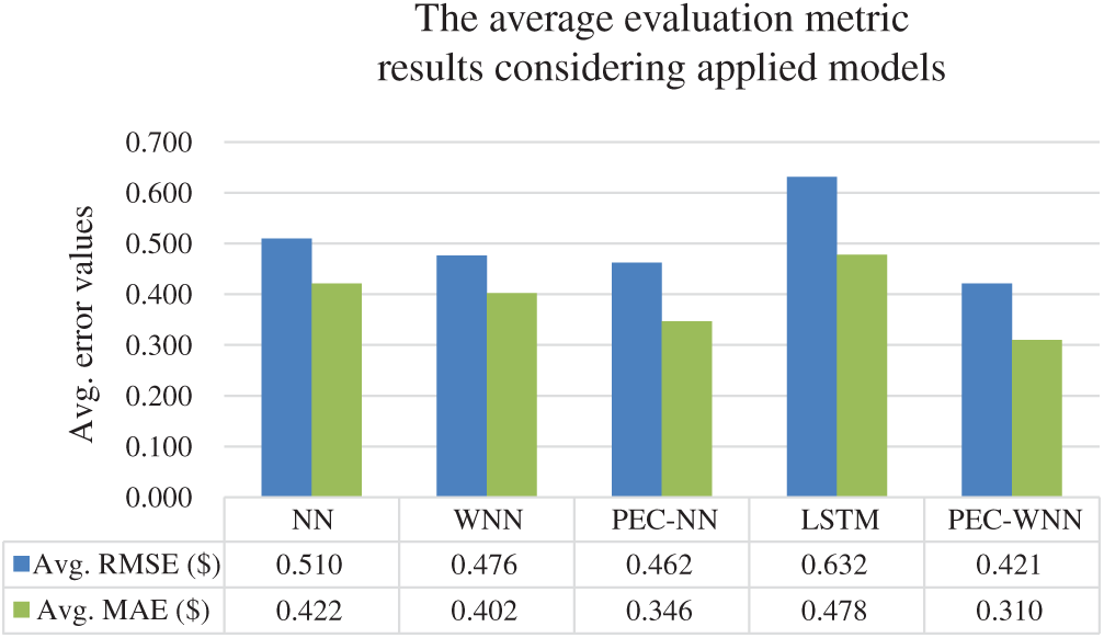
Figure 5: The average evaluation metric results for the multiple time-framed dataset and applied methods
The stock market prediction represents a challenging but important task to analyze the behavior of the financial market. It is important to have accurate predictions to be able to build a profitable financial market transaction strategy. Computationally less complex NN models, using simultaneously different time window past prices are developed to predict the next day closing price using a predictive error compensated wavelet preprocessed model. The proposed method uses in an additive manner two separately trained NN models. The first network performs as the main predictor for the primary estimation of the next day’s closing price. The second network is used for predicting the error of the next day’s closing price. The second network compensates the error of the first one by subtracting the error prediction. The overall prediction performances are improved using the compensation of predicted error through the second NN.
In addition to the proposed model PEC-WNN, four other models were implemented for comparison: simple NN, WNN, PEC-NN, and LSTM. The RMSE error compared to the implemented LSTM model reduces by 53.3% for Apple, 54.9% for Micron, 41.6% for Bank of America, and 42.1% for Ford stocks. The accumulation problem in error feedback neural networks is avoided through independent networks.
An important contribution of this study is the usage of the second network in an additive manner. In this respect, the future study will concern adding additional networks that process additional data for improving the prediction performances.
The second important contribution of this work is the implementation of updated training. The acceptable prediction accuracy can be achieved by applying a fixed training, however with the utilization of updated training the prediction performances can be improved. As another improvement, we will use continual training and update instead of partial repetitive.
The limitation of this article can be seen in considering predictions by closing prices. Future studies may concern data variation patterns inside the session, as well as a larger number of stocks and markets.
Funding Statement: This study is based on the research project “Development of Cyberdroid based on Cognitive Intelligent system applications” (2019–2020) funded by Crypttech company (https://www.crypttech.com/en/) within the contract by ITUNOVA, Istanbul Technical University Technology Transfer Office.
Conflicts of Interest: The authors declare that they have no conflicts of interest to report regarding the present study.
1. https://www.forbes.com/sites/bethkindig/2020/04/10/new-age-of-stock-market-volatility-driven-by-machines/#69dafe996dda, last visit: 09.10.2020. [Google Scholar]
2. H. White, “Economic prediction using neural networks: The case of IBM daily stock returns,” in IEEE 1988 Int. Conf. on Neural Networks, San Diego, CA, USA, vol. 2, pp. 451–458, 1988. [Google Scholar]
3. F. Chague, R. De-Losso and B. Giovannetti, “Day trading for a living?,” Working Paper, 2020. [Online]. Available: SSRN: https://ssrn.com/abstract=3423101 or http://dx.doi.org/10.2139/ssrn.3423101. [Google Scholar]
4. B. M. Barber, Y. T. Lee, Y. J. Liu and T. Odean, “The cross-section of speculator skill: Evidence from day trading,” Journal of Financial Markets, vol. 18, pp. 1–24, 2014. https://doi.org/10.1016/j.finmar.2013.05.006. [Google Scholar]
5. D. J. Jordan and J. D. Diltz, “The profitability of day traders,” Financial Analysts Journal, vol. 59, no. 6, pp. 85–94, 2003. [Google Scholar]
6. B. M. Henrique, V. A. Sobreiro and H. Kimura, “Stock price prediction using support vector regression on daily and up to the minute prices,” Journal of Finance and Data Science, vol. 4, no. 3, pp. 183–201, 2018. [Google Scholar]
7. E. F. Fama and K. R. French, “Common risk factors in the returns on stocks and bonds,” Journal of Financial Economics, vol. 33, no. 1, pp. 356, 1993. [Google Scholar]
8. B. G. Malkiel and E. F. Fama, “Efficient capital markets: A review of theory and empirical work,” Journal of Finance, vol. 25, no. 2, pp. 383–417, 1970. [Google Scholar]
9. L. Bachelier, “Theory of speculation,” in Scientific Annals of the École Normale Supérieure, Serie 3, vol. 17, pp. 21–86, 1900. [Online]. Available: http://www.numdam.org/item/ASENS_1900_3_17__21_0/. [Google Scholar]
10. P. H. Cootner, “The random character of stock market prices,” Louvain Economic Review, vol. 31, no. 8, pp. 733, 1965. [Google Scholar]
11. E. F. Fama, “The behavior of stock-market prices,” Journal of Business, vol. 38, no. 1, pp. 34–105, 1965. [Google Scholar]
12. M. G. Novak and D. Veluscek, “Prediction of stock price movement based on daily high prices,” Quantitative Finance, vol. 16, no. 5, pp. 1–34, 2015. [Google Scholar]
13. Y. S. Abu-Mostafa and A. F. Atiya, “Introduction to financial forecasting,” Applied Intelligence, vol. 6, no. 3, pp. 205–213, 1996. [Google Scholar]
14. J. Bollen, H. Mao and X. Zeng, “Twitter mood predicts the stock market,” Journal of Computational Science, vol. 2, no. 1, pp. 1–8, 2011. [Google Scholar]
15. G. E. Box, G. M. Jenkins, G. C. Reinsel and G. M. Ljung, Time Series Analysis: Forecasting and Control. Hoboken, New Jersey, United States: John Wiley & Sons, 2015. [Google Scholar]
16. J. H. Wang and J. Y. Leu, “Stock market trend prediction using ARIMA-based neural networks,” in Proc. of the IEEE Int. Conf. on the Neural Networks: 4, Washington, DC, USA: IEEE, pp. 2160–2165, 1996. [Google Scholar]
17. M. Aidan, G. Kenny and T. Quinn, “Forecasting Irish inflation using Arima models,” in Technical Paper Ser., Dublin: Central Bank of Ireland, vol. 98, pp. 1–49, 1998. [Google Scholar]
18. R. Nochai and T. Nochai, “ARIMA model for forecasting oil palm price,” in Proc. of the 2nd IMT-GT Regional Conf. on Mathematics, Statistics and Applications, Penang, Malaysia, pp. 1–7, 2006. [Google Scholar]
19. C. Viswanatha Reddy, “Predicting the stock market index using stochastic time series Arima modeling: The sample of BSE and NSE,” 2019. [Online]. Available: SSRN: https://ssrn.com/abstract=3451677 or http://dx.doi.org/10.2139/ssrn.3451677. [Google Scholar]
20. A. A. Adebiyi, A. O. Adewumi and C. K. Ayo, “Stock price prediction using the ARIMA model,” in Proc. of the UKSim-AMSS Sixteenth Int. Conf. on Computer Modeling and Simulation, Cambridge, UK: IEEE, pp. 106–112, 2014. [Google Scholar]
21. M. Khashei and M. Bijari, “An artificial neural network (p, d, q) model for time series forecasting,” Expert Systems with Applications, vol. 37, pp. 479–489, 2010. [Google Scholar]
22. K. Hornik, M. Stinchcombe and H. White, “Multilayer feedforward networks are universal approximators,” Neural Networks, vol. 2, no. 5, pp. 359–366, 1989. [Google Scholar]
23. A. Lendasse, E. de Bodt, V. Wertz and M. Verleysen, “Non-linear financial time series forecasting-application to the Bel 20 stock market index,” European Journal of Economic and Social Systems, vol. 14, no. 1, pp. 81–91, 2000. [Google Scholar]
24. H. Md Rafiul, B. Nath and M. Kirley, “A fusion model of HMM, ANN, and GA for stock market forecasting,” Expert Systems with Applications, vol. 33, pp. 71–80, 2007. [Google Scholar]
25. J. J. Wang, J. Z. Wang, Z. G. Zhang and S. P. Guo, “Stock index forecasting based on a hybrid model,” Omega, vol. 40, no. 6, pp. 758–766, 2012. [Google Scholar]
26. E. Hajizadeh, A. Seifi, A. M. F. Zarandi and I. B. Turksen, “A hybrid modeling approach for forecasting the volatility of S&P 500 index return,” Expert Systems with Applications, vol. 39, no. 1, pp. 431–436, 2012. [Google Scholar]
27. J. T. Yao, C. L. Tan and H. L. Poh, “Neural networks for technical analysis: A study on KLCI,” International Journal of Theoretical and Applied Finance, vol. 2, no. 2, pp. 221–241, 1999. [Google Scholar]
28. A. A. Adebiyi, A. O. Adewumi and C. K. Ayo, “Comparison of ARIMA and artificial neural networks models for stock price prediction,” Journal of Applied Mathematics, vol. 2014, no. 1, pp. 7, 2014. http://dx.doi.org/10.1155/2014/614342. [Google Scholar]
29. M. Nitin, V. P. Saxena and K. R. Pardasani, “A comparison between hybrid approaches of ANN and ARIMA for Indian stock trend forecasting,” Business Intelligence Journal, vol. 3, pp. 23–43, 2010. [Google Scholar]
30. K. Lee, S. Yoo and J. Jongdae, “Neural network model versus SARIMA model in forecasting Korean stock price index (Kospi),” Issues in Information System, vol. 8, no. 2, pp. 372–378, 2007. [Google Scholar]
31. T. B. Shahi, A. Shrestha, A. Neupane and W. Guo, “Stock price forecasting with deep learning: A comparative study,” Mathematics, vol. 8, pp. 9, 2020. [Google Scholar]
32. W. Bao, J. Yue and Y. Rao, “A deep learning framework for financial time series using stacked autoencoders and long-short term memory,” PloS ONE, vol. 12, no. 7, pp. e0180944, 2017. [Google Scholar]
33. J. Li, H. Bu and J. Wu, “Sentiment-aware stock market prediction: A deep learning method,” in Proc. of the Int. Conf. on Service Systems and Service Management, Dalian, China: IEEE, pp. 1–6, 2017. [Google Scholar]
34. I. Goodfellow, Y. Bengio, A. Courville and Y. Bengio, Deep Learning: 1. Cambridge: MIT Press, 2016. [Google Scholar]
35. N. Srivastava, G. Hinton, A. Krizhevsky, I. Sutskever and R. Salakhutdinov, “Dropout: A simple way to prevent neural networks from overfitting,” Journal of Machine Learning Research, vol. 15, no. 56, pp. 1929–1958, 2014. [Google Scholar]
36. https://finance.yahoo.com/, last visit: 13.10.2020. [Google Scholar]
37. B. B. Ustundag and A. Kulaglic, “High-performance time series prediction with predictive error compensated wavelet neural networks,” IEEE Access, vol. 8, pp. 210532–210541, 2020. [Google Scholar]
38. H. B. Hwarng, “Insights into neural-network forecasting of time series corresponding to ARMA (p, q) structures,” Omega, vol. 29, no. 3, pp. 273–289, 2001. [Google Scholar]
39. S. Moshiri and C. Norman, “Neural network vs. econometric models in forecasting inflation,” Journal of Forecasting, vol. 19, no. 3, pp. 201–217, 2000. [Google Scholar]
40. D. W. Patterson, Artificial Neural Networks: Theory and Applications. New Jersey, United States: Prentice-Hall, 1996. [Google Scholar]
41. J. Arnerić, T. Poklepović and Z. Aljinović, “GARCH based artificial neural networks in forecasting conditional variance of stock returns,” Croatian Operational Research Review, vol. 5, no. 2, pp. 329–343, 2014. [Google Scholar]
42. E. Ogasawara, L. C. Martinez, D. De Oliveira, G. Zimbrão, G. L. Pappa et al., “Adaptive normalization: A novel data normalization approach for non-stationary time series,” in Int. Joint Conf. on Neural Networks, Barcelona, Spain: IEEE, pp. 1–8, 2010. [Google Scholar]
43. S. G. Mallat, “A theory for multiresolution signal decomposition: The wavelet representation,” IEEE Transactions on Pattern Analysis and Machine Intelligence, vol. 11, no. 7, pp. 674–693, 1989. [Google Scholar]
44. C. J. Willmott and K. Matsuura, “Advantages of the mean absolute error (MAE) over the root mean square error (RMSE) in assessing average model performance,” Climate Research, vol. 30, no. 1, pp. 79–82, 2005. [Google Scholar]
45. D. Roberts, “Lorenz trajectories prediction: Travel through time,” arXiv preprint arXiv: 1903.07768, 2019. [Google Scholar]
The RMSE, MAPE, and MAE errors for 1. Apple, 2. Micron, and 3. Bank of America.
1. Apple
Table 11: RMSE ($) for predictions of Apple stock prices
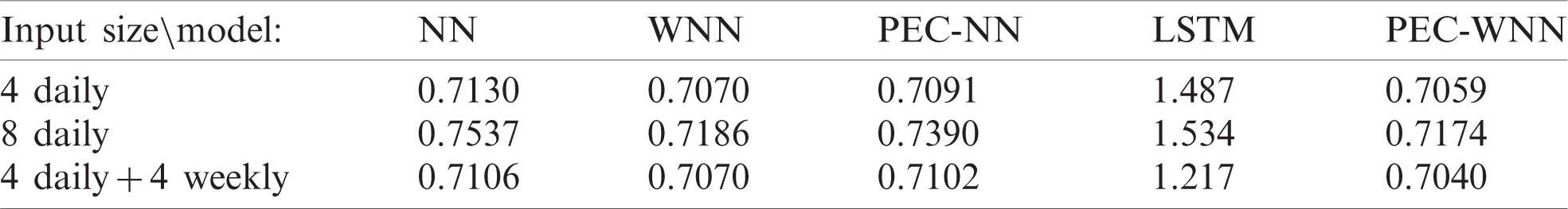
Table 12: MAPE (%) for predictions of Apple stock prices

Table 13: MAE ($) for predictions of Apple stock prices
2. Micron
Table 14: RMSE ($) for predictions of Micron stock prices
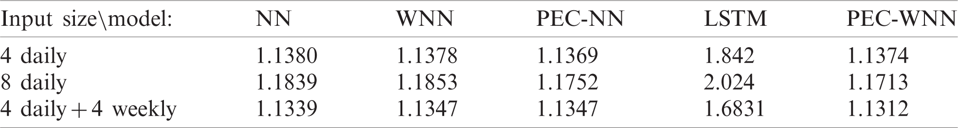
Table 15: MAPE (%) for predictions of Micron stock prices
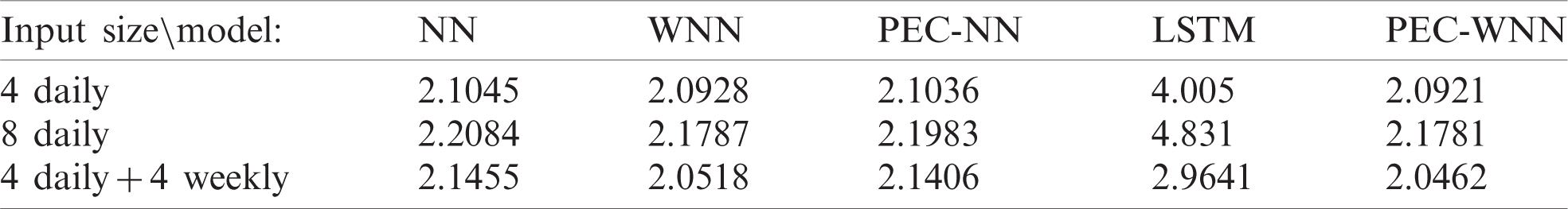
Table 16: MAE ($) for predictions of Micron stock prices
3. Bank of America
Table 17: RMSE ($) for predictions of Bank of America stock prices

Table 18: MAPE (%) for predictions of Bank of America stock prices
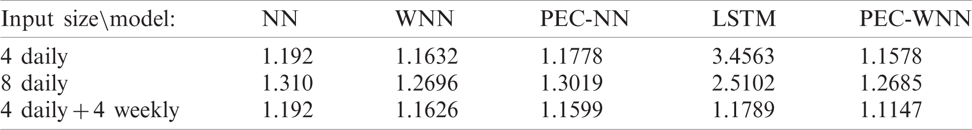
Table 19: MAE ($) for predictions of Bank of America stock prices
 | This work is licensed under a Creative Commons Attribution 4.0 International License, which permits unrestricted use, distribution, and reproduction in any medium, provided the original work is properly cited. |