DOI:10.32604/cmc.2021.015038
| Computers, Materials & Continua DOI:10.32604/cmc.2021.015038 | |
| Article |
Energy Efficient Clustering Protocol to Enhance Network Lifetime in Wireless Sensor Networks
1Department of Computer Science and Engineering, Sri Ramakrishna College of Engineering, Perambalur, 621113, India
2Department of Information Technology, K.S.R College of Engineering, Tiruchengode, 637215, India
3Department of Computer Science and Engineering, PSN College of Engineering and Technology, Tirunelveli, 627152, India
*Corresponding Author: S. Nanthini. Email: nanthiniresearchscholar@gmail.com
Received: 03 November 2020; Accepted: 04 March 2021
Abstract: In this paper, the energy conservation in the ununiform clustered network field is proposed. The fundamental reason behind the methodology is that in the process of CH election, nodes Competition Radius (CR) task is based on not just the space between nodes and their Residual Energy (RE), which is utilized in Energy-Aware Distributed Unequal Clustering (EADUC) protocol but also a third-degree factor, i.e., the nearby multi-hop node count. In contrast, a third-factor nearby nodes count is also used. This surrounding data is taken into account in the clustering feature to increase the network’s life span. The proposed method, known as Energy Conscious Scattered Asymmetric Clustering (ECSAC), self-controls the nodes’ energy utilization for equal allotment and un-equal delivery. Besides, extra attention is agreed to energy consumption in the communication process by applying a timeslot-based backtracking algorithm for increasing the network’s lifetime. The proposed methodology reduces the clustering overhead and node communication energy consumption to extend the network’s lifetime. Our suggested method’s results are investigated against the classical techniques using the lifetime of the network, RE, alive hop count and energy consumption during transmission as the performance metric.
Keywords: Wireless sensor networks; energy conservation; lifetime enhancement; clustering; cluster head
Wireless Sensor Networks (WSNs) are unique with more source restrictions like energy, the power to process, accumulation and communication range. Among the criteria, sensor energy is the critical resource limitation of the WSNs. Many research types have been studied to fix this issue [1,2]. Nodes in WSN are placed very close to collect data in applications that require huge areas like farming, jungle, mining, monitoring rail tunnels, the solar cell in a grid etc. They need information from all positions [3–5].
In most cases, the Base Station (BS) is located faraway from the detecting area. In those networks, BS regularly collects the information. To get consistent monitoring networks, it is very fruitful to cluster them with classified topology. It was shown that the clustering of the network provides more life for the network than the one with transmitting information straight away. It was seen that the network shelf life becomes better twice or thrice with clustering [6,7]. In clustering, the sleep times of the usual SNs (Sink Node) are defined, whereas Cluster Heads (CHs) organize the fellow nodes’ action, once again leading to control of energy consumption [4,8,9].
Moreover, clustering aids’ collection of information at CH by reducing the count of data packets being transmitted, aids in minimizing the consumption of energy in sensor nodes [10,11]. This process is done in a couple of stages, (1) intra-cluster, which means clustering within itself, (2) inter-cluster, which means clustering amid cluster and BS. Besides, the WSN clustering scheme’s exchange of messages is assimilated either with an SH transmission or MH routing. For the exchange of messages within-cluster, the majority of the clustering protocols use Single-Hop (SH) communication because, within the cluster, the space amid sensors is comparatively shorter, e.g., LEACH-DT [8], LEACH [12], HEED [13–15], etc. Previous studies show that multi-hop interaction amid the SNs and the CH is highly economical in energy compared to the single hop interaction while losing the broadcast.
The Multi-Hop (MH) communication works well in handling the downfalls in signal propagation because the radio loses energy not just while transmitting but also while receiving messages; transmitting straight away is even helpful. Yet, the occurrence of restriction is present here. It is fair to utilize it up to some distance only [16,17]. Because of the reason being, when it comes to the extent of transmitting above the saturation point, the usage of energy raises based on the 4th power of the distance [8]. Hence, to increase the network’s expansion, MH communication is most sought over [18,19]. When it comes to communication from the CH node to the BS and if BS is at a distance from the sensor field, it is improved by utilizing MH neighbourhood node communication. A CH is severely overloaded with clustering protocol because it has to do different work like forming clusters, aggregating information, transmitting information and relaying. CHs, hence use more energy than other non-CH nodes. While sending inter-clusters for the two modes of communication viz., SH and MH, there is an unavoidable energy issue, not balancing amid SNs. For SH communication, CHs placed at a distance from BS use most of their energy primarily due to longer transmission.
Losing the sensing coverage and dividing the network happen, finally influencing the functioning of the network. In the literature [20], it has been shown that when sensors get arranged consistently in the area of concern, they leave around 90% of the sensors’ total energy not used until the first Node is dead. The inevitability of the ununiform decrease in energy among the entire sensors in WSNs was confirmed in [21,22] as the many-to-one transmission model. To get a maximum lifetime of the network, energy consumption must be balanced amid all network nodes. Many research studies have been done to fix the unequal energy and simulate the energy deficit issue for clustered WSNs. Schemes like using node mobility, mobile sink, hierarchical deployment, non-uniform clustering, data compression, traffic aggregation, node distribution etc., were suggested to fix the energy deficit issue.
The surrounding information is taken into account as the clustering parameter to improve the network’s life span. The proposed method, ECSAC, self-controls the energy usage by the nodes in the network for equal distribution and un-equal delivery. Besides, extra attention is given to energy consumption in the communication process by applying a timeslot-based backtracking algorithm for increasing the network’s lifetime. Ultimately, the suggested algorithms minimize the transceiver’s energy expenditure consumption by fixing the issues mentioned above. Our methodology reduces the clustering overhead and node communication consumption to extend the network’s lifetime. The output of our suggested method is analyzed against the classical techniques under various performance metrics.
Zhu et al. [23] put forth a tree-cluster-based information collecting algorithm with a mobile sink. The tree is designed for every sensor node by considering the mean leftover energy, location concerning the sink, and nodes count in the location. Djenouri et al. [24] suggested a trustworthy estimator algorithm for enhancing the Packet Reception Ratio (PRR) of the link relaying Node vi to node vj. The PRR specifies the probable positive delivery over the link. Badia et al. [25] have chosen the joint link scheduling and routing algorithm for delivering the packets under the time limit with actual intrusions amid nodes. On the contrary, the genetic algorithm increases throughput, fine-tunes transmission power, channel assignment and route path selection in Jia et al. [26]. The algorithms, as mentioned earlier, are not taking into account the sensor node energy and the network lifetime enhancement.
A low-complexity distributed clustering scheme was proposed by [27] for Machine-to-Machine (M2M) interactions in Long Term Evolution (LTE) networks for increasing the battery life of nodes. The location of the BS is crucial in optimizing the network. Therefore, [28] analyzed the chances for several BSs and locations of BSs, which could increase the life of WSNs. Here, the sensor nodes probably minimize energy consumption. Likewise, low-complexity solutions for enhancing network performance are suggested by [29], taking into account the available information during routing, planning, and frequency band allotments link. The density of Node influences the shelf life of the network. A cross-layer mathematical model was created by [30] to find the best node density for maintaining correct energy usage for every bit transmission. Augmentation of network life is possible by saving the source node’s position and ignoring the hot-spot Node. A routing algorithm created by [31] has various routes overlooking hot spot regions by attaining network life increment and generating repeated distracting routes in non-hotspot places with excess energy.
The Energy-Driven Unequal Clustering protocol (EDUC) methods [32] for a scattered non-uniform Clustering Algorithm (CA) and a dynamic adaptive CH alternation technique. Here, CH alternation’s energy utilization is reduced by permitting a node to be CH once in the network’s lifetime. Therefore, when the energy spent in CH alternation is minimized, energy efficacy is attained. Nevertheless, there is a restriction here, which is beneficial for SH networks only. In the technique named Unequally Clustered Multi-hop Routing protocol (UCMR) proposed by [33], every cluster comes in various dimensions according to the radii and Dijkstra’s shortest path algorithm that aides in the communication of within and outside the cluster. UCMR is quite different from others as it depends on accurate place information. The disparity in energy issues through energy- and proximity-based unequal CA (EPUC) is discussed in [34]. Excess energy and closeness to BS determine the selection of CHs. Attention is more on the zone close to BS to tackle the disparity in energy as the region requires more energy due to relaying activity.
HEED and EEDC, a couple of energy-efficient distributed CAs, were put forth in [35] and [36]. In this algorithm, sensor nodes are chosen as CHs. Yet, both of them do not consider the “energy hole” issue. As a solution to this issue, Soro et al. [37] suggested an unequal CA where the network zone is separated into cirques. Clusters in one cirque have similar dimensions, whereas unlike clusters in several cirques have, unlike aspects. High energy nodes usage for handling the CH role, thereby controlling the process of network, assures that the energy consumption of these CHs is controlled. This, in turn, enhances the lifetime of the network. Nevertheless, this requires specific high-energy nodes as CHs he placement of CHs is to be ascertained in advance. EEUC [38] is yet another distributed unequal CA. It chooses CHs according to the Node’s unwanted energy. There is a possibility for every Node to develop into a CH with a probability T. These probable CHs utilize uneven competition ranges for building unequal dimensions. Distance from the BS determines the cluster size. Closer is smaller than the ones at a distance. This results in the energy-saving by the CHs, which is closer to BS for the data communication between clusters. This leads to the balancing of energy consumption amid CHs. T affects the efficiency of collected CHs; hence, the presence of “isolate points” in EEUC. [39] proposed Enhanced Hybrid Multipath Routing (EHMR) to ensure energy efficiency and enhance fast failure recovery. Reliability is ensured in terms of maximum data rate and the minimum end-to-end delay.
The network used in this model has ‘Nd’ no. of SNs arranged haphazardly in an S × S sensor field. Once the arrangement is made, the nodes and the stations turn immobile—the Node’s different energy ranges, i.e., the nodes used with various primary energy. The BS is placed at a distance from the sensor field, and its position is taken to aware of every Node. The nodes use power regulation for adjusting the power required for transmitting based on the distance. The views are not known to the nodes, but the nodes capable of calculating the space between two nodes are formed on the signal’s strength; the links are considered symmetric. The CHs are capable of transmitting their information straight away to the BS. The data (DMsg) and control (CMsg) are sent via wireless links.
Moreover, we presume that the information detected by the nodes is strongly related. Once the cluster has been formed, DG gives the election of Cluster Head in WSN = (Sn, Ed). Here, Sn means that ‘N’ wireless SNs are along with the CH. Not including the Node acting as sink Sns., every SN Sni regularly produces size k. In Ed, (Sni,Snj) is the pair of guided edges, where Sni,Snj as the child and the parent node. The edge’s direction Sni→Snj indicates that in which way the information is being forwarded. The edges represent the information that performs the transmission of a spanning tree with the Sink Node (SN) as an origin. It assumes that backing of various radio frequencies for simultaneous interactions sans intrusion is performed by manufacturing, technical, health care band, etc. Allotting RF channels for a bunch of synchronous communications is NP-Hard. Therefore, the suggested method presumes that the network is present with the highest S RF channels. The following Fig.1 indicates a routing graph of an SN with 25 SNs.
The transmitter used energy to run and transmit the radio electronics circuit, but the energy of the recipient was in the component of the radio electronics alone. Furthermore, the free space φfs and the multipath fading φmp model channels are used depending on the propagation’s significant degree. The open space model is used or the multi-route model used if the travel time is less than the limit. The transmitter spends energy based on Eq. (1) during transmission of the n-bit data to the range k.
The transmitter then spends energy for receiving n-bit of data based on the following Eq. (2)
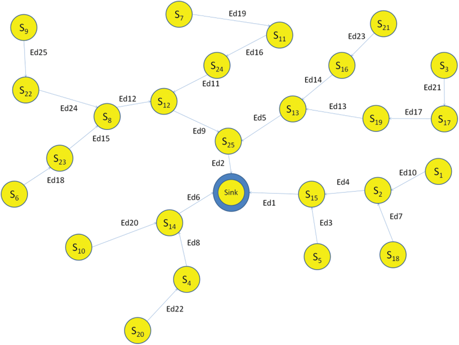
Figure 1: Network routing graph
In this suggested methodology, the TDMA method categories into a group of small timeslots of uniform distance end to end. Every cluster node is allotted a timeslot that regularly forwards a combined data packet to the CH in the allocated time.
As per Fig. 2, the same timeslot is employed for the forwarding node for the Trx process when utilized for the Rex functioning in the respective gathering (parent) Node. With a channel alteration time, the timeslot starts, and for forwarding, it is kept as the minimum time to swap the channel to a different channel assigned. Meantime, a device cannot transmit or receive any packet. Apart from this, Trx operation consists of synchronization margin time (Sync), Carrier Sensing Time (CST), Trx data interval (the time needed for the huge data packet to be received), and Rx Ack interval (requirement of time for obtaining back from the parent, an acceptance packet).
Researchers have detailed the accumulation methodologies for a couple of strong cases of compressing without the information (raw-data forwarding) in addition to compressing complete data (aggregated forwarding). They are compressing without information forwards data packets created by every Node separately. On the other hand, in the other type, the data obtained from every Node of the sub-tree is combined into a uniform size packet by the root node. Later, just a combined packet from the sub-tree’s root node is transmitted. Once a robust geological correlation is obtained by the data, the combined forwarding is used or gathering brief data like the highest, lowest or mean is the aim. In our research work, we suggest a novel combination method in which the root node of every sub-tree joins the sensing information obtained from every Node in the sub-tree with its data.
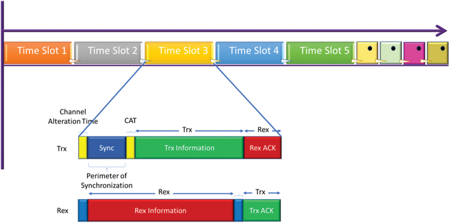
Figure 2: Allotment of timeframe into time slots
In our methodology, the parent node is assigned by a routing protocol to the extent that the following limitation is fulfilled. Let every Node make a ‘l’ sized sensing data, and ‘hd’ be the header’s size. Next, Eq. (3) calculates the combination of the gathered packet’s data size for any node ‘sn’.
As per Eq. (4), the aggregated packet’s dimension must not go beyond the largest packet maxl that could be conveyed in the Trx information of one timeslot gap.
4.1 Cluster Formation Using Energy-Conscious Scattered Asymmetric Clustering (ECSAC)
The nodes’ distance from BS is first calculated once they are placed. To accomplish this, an indication is transmitted by BS, and the entire nodes could hear it. Every Node consolidates the distance of sits with BStn by the obtained indicator’s power. Every round contains a cluster establishment stage and a firm-state stage, where data diffusion happens. To have a clustering topology, the establishment stage is categorized into three sub-stages: fellow node spec gathering phase, CH selection phase and cluster creation stage. In the information forwarding stage, cluster members gather information within the surroundings and transmit the collected information to the CHs that receive and combine the data from their fellow clusters and then forward the combined information to the next-hop nodes according to the routing tree designed in this model.
Table 1: Narrative of node state messages
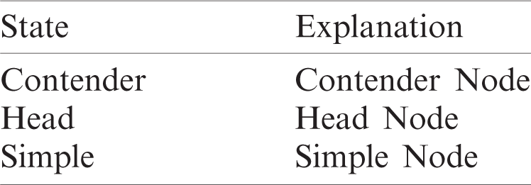
Table 2: Narrative of control messages
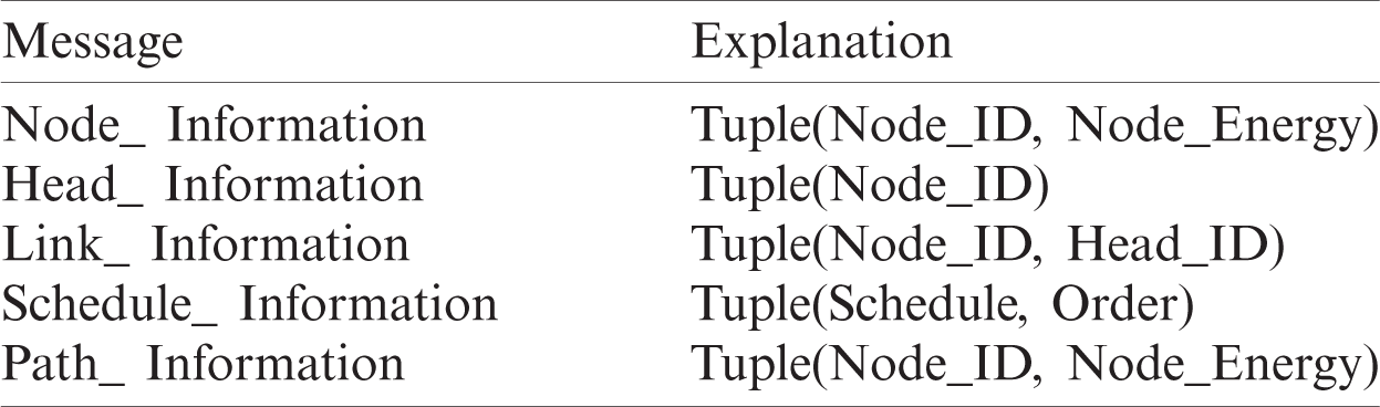
The data transmission, which is a firm-state phase, must be longer than the establishment phase for preserving the algorithm’s overhead and extending the network lifetime. The state message of every Node is mentioned in Tab. 1. Many control messages are required, and the explanation of these messages is shown in Tab. 2.
4.2 Cluster Establishment Stage
4.2.1 In the NETWORK Deployment Stage
The BS transmits a signal at a particular power range. Every Node can work out its position corresponding to the BS according to the strength of the signal received. There are three sub-stages in cluster setup phases: fellow node spec gathering stage, where duration is T1; CH choosing stage, where the period is T2; cluster formation stage, where the period is T3.
In the Fellow node spec gathering stage, every Node transmits Node information within radio r with the below mentioned two values: the node id and its remaining energy Rnrg. Simultaneously, it gets the Node_ information’s from the nearby nodes, based on which every Node determines the avg. and the remaining energy of its nearby nodes Rnrgavg using the following Eq. (5):
where
where
For any node nid here, it gets no Head_ information when Tc expires, and it transmits the Head_ information within radio range RRi to showcase that it will be a CH. Or else, it retires from the competition. To not create such equal clusters, every Node has to compute its CRRR. The formula of RR in Li et al. [38] is given in Eq. (7):
where maxd and minds are the max and min space between the nodes in the network and the BS, d(nid, BS) is the distance from node nid to the BS, ω is a weighted factor whose value is in [0,1] and
The ECSAC system is according to the improved EADUC methodology, but contrary to the EASAC scheme, for producing unequal clusters, it uses a different CR rule. Only the distance between nodes and BS are taken into account in the original EADUC protocol for the expression of CR and the RE of nodes. Therefore, the suggested scheme addresses, apart from the latter two considerations, the amount of neighbors and calculates the radii rivalry to compensate the costs involved in the aggregation. The strategic range is the distance from the BS, CH’s remaining strength, and adjacent nodes’ count. The suggested scheme nodes with comparatively more remaining power, a total distance of nodes from the BS, few neighbouring nodes, etc., should have a more comprehensive broader range of competition and the formula given in Eq. (8) is used to accomplish this.
In heterogeneous networks, nodes have different initial energy. Here, every Node has equal energy consumption, and the nodes with minimal initial energy fall off early, thereby decreasing the lifetime of the network. To have the full benefits of the high-energy nodes, the high-energy nodes must accept more tasks. Hence, taking into account the gap amid nodes, the BS and the RE of nodes, we derive the formula of Rr:
where
(i) Cluster Construction Phase. It is the last sub-phase of the cluster association phase. Every non-cluster-head Node selects the closest CH and transmits the Join_ information with the id and leftover energy. According to the received Join, every CH generates a node plan list and sends it to the fellow members by transmitting Schedule Msg.
(ii) Data Transmission Phase. The stage during which information is transmitted has numerous significant slots. Each primary slot has many rounds, a CH alternation and an alteration route. Two stages create them: (a) intra-clustered forwarding of information and (b) inter-clustered forwarding of information
(a) Intra-cluster forwarding of information
In the intra-cluster communication process, all the nodes present within the cluster sense their local environment and collect it. Each Node then forwards the gathered information to their corresponding CHs. The CH sums up the received message and transmits the packet to the SN with the help of inter-cluster communication
(b) Inter-cluster forwarding of information
The CHs aggregate the data that had been obtained from its nodes. The aggregated data are then forwarded to the SN. The management of inter-cluster communication is essential as it alone utilizes the central part of any sensor network’s aggregate RE level.
In this model, a backtrack-based channel allocation is employed to ensure better energy management among the CHs. The scheduling algorithm presented here discovers maximum possible ways with the help of backtracking—the algorithm CATUB receives an allocation solution with less energy consumption. A pseudo-code CATUB is depicted by Algorithm 1. The algorithm inputs are G = (V, E), the directed routing graph and S, the maximum No. of channels available. For each sensor node, the algorithms produce a communication Allocate [T][C]. Here, the Node assigned with an ith timeslot and the jth channel is represented by the values in Allocate [i][j]. To gather the sensing information from entire nodes at the sink (root) node atone time, Child node timeslots should be allocated before their origin node timeslot. Therefore, the algorithms begin by assigning the schedule in a bottom-up style from the leaf nodes towards the SN.
4.2.2 Channel and Timeslot Allocation using Backtracking (CATUB)
CATUB preserves the lowest energy solution in Allocate [T] [C] available post recursive function calls. Backtracking tree schedule’s present situation is hoarded in PrsnSolu [T][C]. For memorization, the plan of the present example’s cost metric is hoarded by the algorithm in NrSolu. Allocate [T] [C]’s minimum energy cost is hoarded in Nrmin. Eq. (9) shows the obtained cost metric about the aggregate of the forwarding, getting and stagnant power consumed for every Node network.
The values
In every resolution, the algorithm gets a schedule and channel provision to the entire nodes before the algorithm attained the SN. It is done when the current answer has a small cost metric compared to the former top solution (Nrsolu < Nrmin) and the algorithm stores both cost Nrsolu and scheduling outcome PrsnSolu[T][C] into Nrmin
Input:
1. A directed graph, Dg = (Sn, Ed), where Sn is the vertices that represent the representing SN and Ed represent the edges of the directed graph.
2. Set of maximum available channels Cmax.
3. The least found energy solution available recently, Nrmin.
4. A 2D array Allocate [T][C] that could store the results. The Allocate[t][c] represents that a node is allotted a timeslot t to transmit the aggregated data through the given channel c.
5. Nrsolu, the current energy consumption level.
6. Prsnsolu[T][C] stores the scheduling parameter for the current energy consumption level Nrsolu.
7. ReadyQ holds the list of nodes that are available to be scheduled in the next timeslot.
8. IdleQ holds the record of nodes in idle mode waiting in the present time slot.
9. Timeslot, the implementation of present timeslot.
Output:
1. Allocate [T][C], which specifies the transmission-schedule for all the nodes in Sn.
Initialization:
1. Nrmin = ∞
2. Nrsolu= 0
3. ReadyQ = Enqueue (n ∈ Sn|n.Child → 0)
4. IdleQ = ∅
5. Timeslot = 0
Function (Recursive)
Allocate_Slot (Timeslot, C, Nrsolu, Nrmin, Prsnsolu[ ][C], Allocate[ ][C], ReadyQ, IdleQ)
1. Valueret = 0
2. If ReadyQ = = ∅
3. If Nrsolu < Nrmin
4. Nrmin= Nrsolu
5. Allocate = Prsnsolu
6. Valueret = 1
7. Else Valueret = 0
8. End If
9.Else If Nrsolu ≥ Nrmin
10. Valueret = 0
11. Else
12. While Prsnsolu[timeslot] = Choose_Allocate_node(ReadyQ) ≠ SINK
13. For n = ∀Prsnsolu[timeslot]
14. ReadyQ =Dequeue(n)
15. IdleQ = Dequeue(n)
16. Nrsolu+= n.NrTrx + n.Parent.NrRex
17. IdleQ = Enqueue(n.Parent)
18. ReadyQ = Enqueue(n.Parent)
19. End For
20. For i = ∀IdleQ
21. For n = ∀Prsnsolu[Timeslot]
22. If n.Parent = i
23. Break
24. End If
25. End For
26. Nrsolu += Nridl
27. End For
28. Valueret = Valueret|Allocate_slot(Timeslot + 1, Nrsolu,Nrmin, Prsnsolu[ ][C], Allocate[ ], ReadyQ, IdleQ.
29. For i = ∀IdleQ
30. For n = ∀Prsnsolu[Timeslot]
31. If n.Parent = i
32. Break
33. End If
34. End For
35. Nrsolu - = Nridle
36. End For
37. For n = ∀Prsnsolu[Timeslot]
38. ReadyQ =Dequeue(n.Parent)
39. IdleQ = Dequeue(n.Parent)
40. Nrsolu - =n.NrTrx + n.Parent. NrRex
41. IdleQ = Enqueue(n)
42. ReadyQ = Enqueue(n)
43. For End
44. End While
45. Return Valueret
46. End If
and Schedule [T] [S], correspondingly. It explains that the present clarification offers a minimum consumption compared to former schemes (Nrsolu < Nrmin). CATUB at first lines up every branching node into the (s ∈S|s.children== 0) into queue ReadyQ that accumulates the nodes, which are ready for getting planned with the setting: (1) the leaf nodes (without child nodes) and (2) priorly scheduled nodes with child nodes. By inviting the Recursive function (RF) from the timeslot 0, the CATUB algorithm begins. RF’s input has two queues: ReadyQ and IdleQ. At first, IdleQ begins as a queue without any nodes. As the branch node is without children, they start quickly in their broadcasting schedule. In every timeslot, the algorithm looks into every possible subset of nodes fulfilling the application limitations. C gives a large-sized subset. In the timeslot, for every queued subset, the algorithm recurrently performs the other nodes that are not in the queue for the following timeslots. Finally, the algorithm comes back to the minimum energy schedule Allocate [T] [C].
As a sample, in the network of Fig. 1, the enqueuing of the leaf nodes Sn5, Sn18, Sn1, Sn6, Sn7, Sn10, Sn3, Sn20, Sn21 and Sn9 to ReadyQ is commenced by CATUB for timeslot T0 to get ready. There is an emptiness in IdleQ, the queue for idle nodes. CATUB finds all likely, probable subsection of nodes, which fulfil the highest channel constraint C = 4 in timeslot T0. Such subsections are (Sn3, Sn9, Sn6, Sn7), (Sn6, Sn7, Sn5, Sn18). The algorithm computes the cost for every subsection and performs with the recent criteria, the recursive job ALLOCATE_SLOT for timeslot T1. The algorithm adds up scheduled Node’s parents to the queue Ready If subsection (Sn3, Sn9, Sn6, Sn7) for timeslot T0 is chosen.
Nodes Sn5, Sn18, Sn1, Sn23, Sn11, Sn10, Sn17, Sn20, Sn21 and Sn22 are the latest queue ReadyQ. To queue IdleQ, the parents of the scheduled nodes, Sn17, Sn22, Sn23, Sn11, are too restructured. When the latest consumption is greater than the former least consumption (1 is the initial minimum cost) value in the T1 timeslot, CATUB performs backtracking to timeslot T0, and the remaining subsets are discovered. When lesser is the latest cost than the legal best cost, the execution of CATUB in the timeslot T1 is done in a similar manner to the one in the timeslot T0. The other timeslots also once again go through a similar process. Tab. 1 details the individual Node’s energy consumption and the duration of a single timeslot. 79.52 mJ is the energy spent on CATUB.
Three conditions were selected for imitations:
Scenario 1: 100 nodes are consistently placed around an area of 300 × 300 m2 as exposed in Fig. 3a.
Scenario 2: 100 nodes are inconsistently placed with more SNs collated together in the area on the right side of the sensor field, i.e., near the BS, around an area of 300 × 300 m2 as depicted in Fig. 3b.
Scenario 3: 100 nodes are inconsistently placed with more SNs and are assembled on the left side of the sensor field, i.e., off from BS, about an area of 300 × 300 m2, as shown in Fig. 3c.
Scenario 4: 100 nodes are inconsistently placed with more SNs brought together in the region in the middle of the sensor field, i.e., little away from BS, around an area of 300×300 m2 as proved in Fig. 3d.
In the methodology put forth in our study, the count of alive nodes, the avg. of network energy and network stability, First Node Death (FND), Half Node Death (HND), destruction of 10% and 20% of nodes (PND) and Last Node Death (LND) in the entire imitation duration were all assessed. The reproduction was performed in 50 periods.
Few are explained below:
• Network Life Span: The period that is the beginning of the network functions to the last node death.
• Network Stability: The period from the beginning of the network functions to first node death.
• Throughput: The No. of data packets. A network transmitted it to the BS. Efficiency enhancement directly links with improved network stability and the network lifetime.
• Load Balancing: Traffic load distribution. Its gain being the load is well-disseminated across the nodes, leading to a balanced consumption of energy. Also, nodes’ unexpected downfall because of their over-usage is avoided, resulting in an enhanced network’s enhanced lifetime.
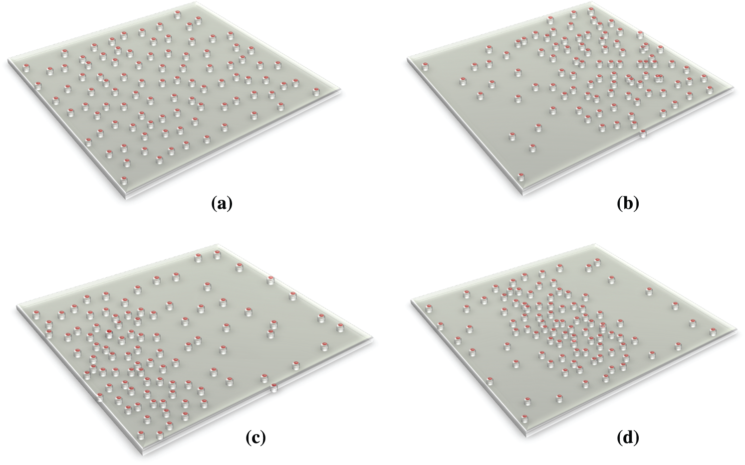
Figure 3: Network topology in the four scenarios. (a) Scenario 1. (b) Scenario 2. (c) Scenario 3. (d) Scenario 4
The factors responsible for replication are shown in Tab. 3. The best No. of some of the parameters (for x.:RLmax) was calculated from different replication outcomes.
The simulations are repeated many times for finding round No. in a significant slot and many slots in the data transmission stage. Replication factors, like the nodes’ positions, are seen as the same for every Node so that the outcomes are reliable and trustworthy. This simulation has got a significant part to play in the suggested method. Here, the simulation could be done more accurately by reducing round count, leading to increased overhead, energy consumption and reduced network lifetime. The project’s critical aim is to raise the life span of the network by removing almost all of the regulation messages and decreasing the overhead, thereby resulting in reduced energy consumption of nodes. As per the simulation results, it is observed that every information forwarding stage has seven parts of the vital slot that has six rounds, one cluster head rotation, and one adjustment route. In general, in the information forwarding stage, information was forwarded in 42 rounds, and our objective was to eliminate most of the network overhead.
One of the essential parameters in clustering is finding the radius. Thus, in Eq. (10), the primary level is equal to 1, in the 2nd and 3rd levels is 1.25, and in the 4th level is 1.75. Therefore, the clusters placed near the BS are smaller, and the cluster head can get additional energy for transmitting and routing other Cluster Head packets to the BS.
For finding the RMRnrg parameter in Eq. (10), many practice tests are done using various RMRnrg values for getting the correct value for the RMRnrg setting. Among the various vital factors, wireless nodes, the No. of CH and the cluster dimensions rely on Node’s radio. The outcome of the simulated runs for multiple situations is presented below.
Table 3: Simulation parameters
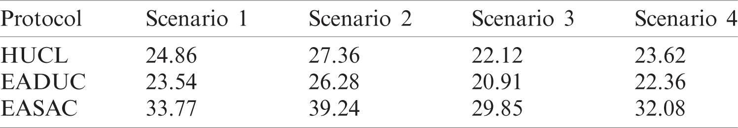
7.1 CH Distribution Evaluation
In this proposed model, the right CH count is calculated to be equivalent to 5% of the network’s entire nodes. Every Node has a distance that has to be such that the No. of clubs in the network must be appropriate. In this case, the parameter’s value RMRnrg was estimated to be equivalent to 100 m, Which implies that CH is around 5. Fig. 4 indicates in every case the mean No. of CHs. The CHs are allocated, and there is also power over the No. of CHs. The below figure shows the EASAC protocol that generates a stable No. 2. This is because of the presence of just one CH in every competition by the competitive radius. For scenarios 1 and 4, i.e., containing standardized dispersed sensors and clustered sensors, 4-5 cluster head Nos. are produced and possibly during each protocol round. Six clusters No. heads are more probable in scenario 3, whereas 4 CHs are more common in scenario 2. The nodes close to BS are allocated smaller competitive radii during the protocol process. As in scenario 2, additional nodes are positioned near BS; more CHs than in scenario 3 are likely to be created in the region near BS.
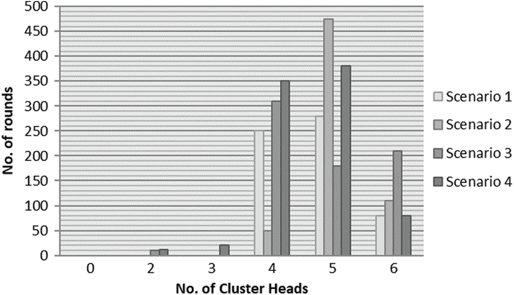
Figure 4: Average number of cluster heads created in dissimilar scenarios
7.2 Estimation of Energy Utilization
The ECSAC, EADUC and HUCL protocol’s mean energy consumption is calculated for the four situations included here. Fig.5 depicts the mean energy consumed in each round in the network when each protocol is functioning until it dies for the 3 types of situations. Energy spent in a round consists of the energy utilized in clustering topography creation and forwarding of information. The low energy consumed in the HUCL process is lower than the EADUC process and is weaker when it comes to the ECSAC process. Moreover, we notice the mean energy consumption of the network in the scenario.
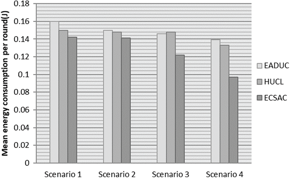
Figure 5: Energy utilization against each scenario
Three is just more than scenario 2; like in scenario 3, the area near the BS vicinity is scarcely organized. Therefore, there is more possibility of a long-distance between the last transmit Node and BS than scenario 2. It is thickly arranged.
7.3 Network Stability and Network Lifetime
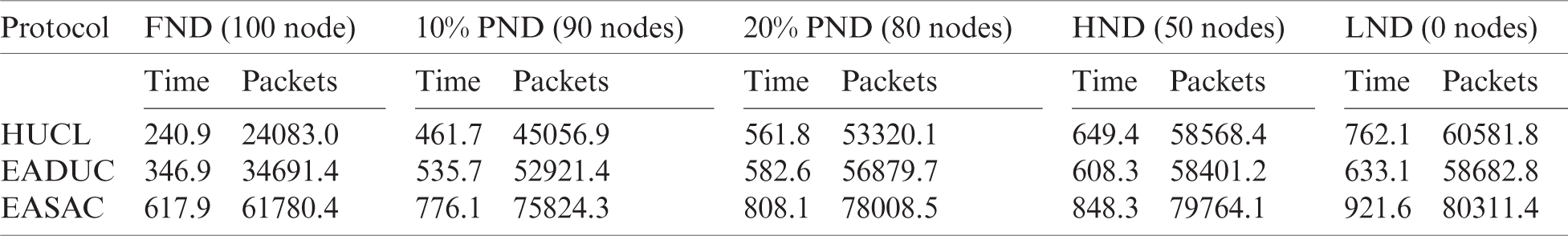
To increase the quality and throughput, additional information to the BS has to be transmitted, and here, it is essential to avoid the Node’s downfall. Hence, efficiency and performance can be enhanced by raising the steadiness of the network. In Tabs. 4 to 7, the output of the stability period and the network lifetime consisting of FND (100 Nodes), 10% PND (90 Nodes), 20% PND (80 Nodes), HND (50 Nodes) and LND (0 Node) of the methodologies were calculated for the primary and secondary situations, where the suggested method performed better than the HUCL and EADUC algorithms. The recommended protocol showed better output with more excellent stability in a range of spaces. ECSAC receives aide from data obtained from the nearby nodes for grouping and uses inter-cluster and intra-cluster as along with MH forwarding correctly. In Tabs. 4 to 7, the outcomes are shown, which explains that the suggested methodology can enhance certain factors and transmit extra packets when there is an incidence of parameters.
Table 4: Simulation outcome of the stability and lifetime for scenario 1
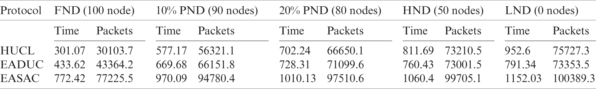
Table 5: Simulation outcome of the stability and lifetime for scenario 2
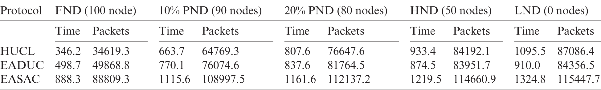
Table 6: Simulation outcome of the stability and lifetime for scenario 3
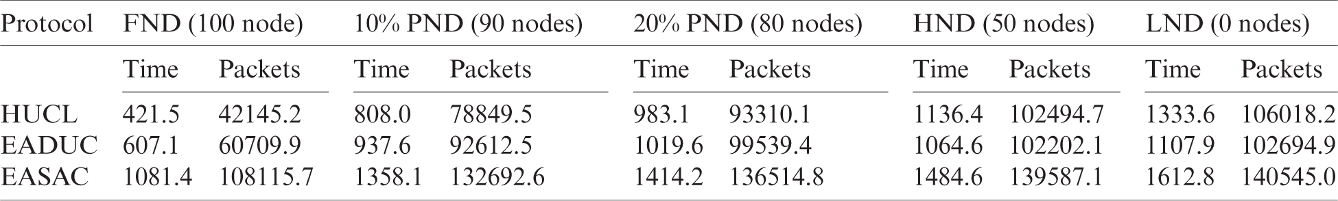
Table 7: Simulation outcome of the stability and lifetime for scenario 4
It was stressed that these nodes without perfect energy levels could not be a CH as they require much energy. Hence, it leads to the division of energy consumption uniformly amid the nodes at simulation time. The protocol put forth assistance in bringing down the energy spent in the network by removing abnormal regulating information and minimizing overhead; hence, it leads to a stretched network lifetime.
Tab. 8 shows the mean no. of live nodes. We can ascertain from this that the mean no. of live nodes went across 38% of all node counts, confirming the sustained network stability suggested by our algorithm. As per our results, ECSAC showcased good results than the rest of the procedures and also raised live nodes to count in simulation. It is all because of the stability amid the energy consumption in various nodes as suggested by preventing node expiry.
Table 8: Average number of living nodes
7.5 Energy Utilization Throughout the Transmission Stage
Post the completion of the forwarding of the collected information packet and every SN changes to the eternity sleep mode until the expected information collection duration. The energy spent in sleep mode is insignificant and not taken into account. The outcome shows that the CATUB algorithm employed in the ECSAC model spends minimum energy. The energy consumption raises proportionately with the network size. The results of the competing models and the proposed model’s energy consumption during the transmission phase are indicated in the following Fig. 6a to 6d.
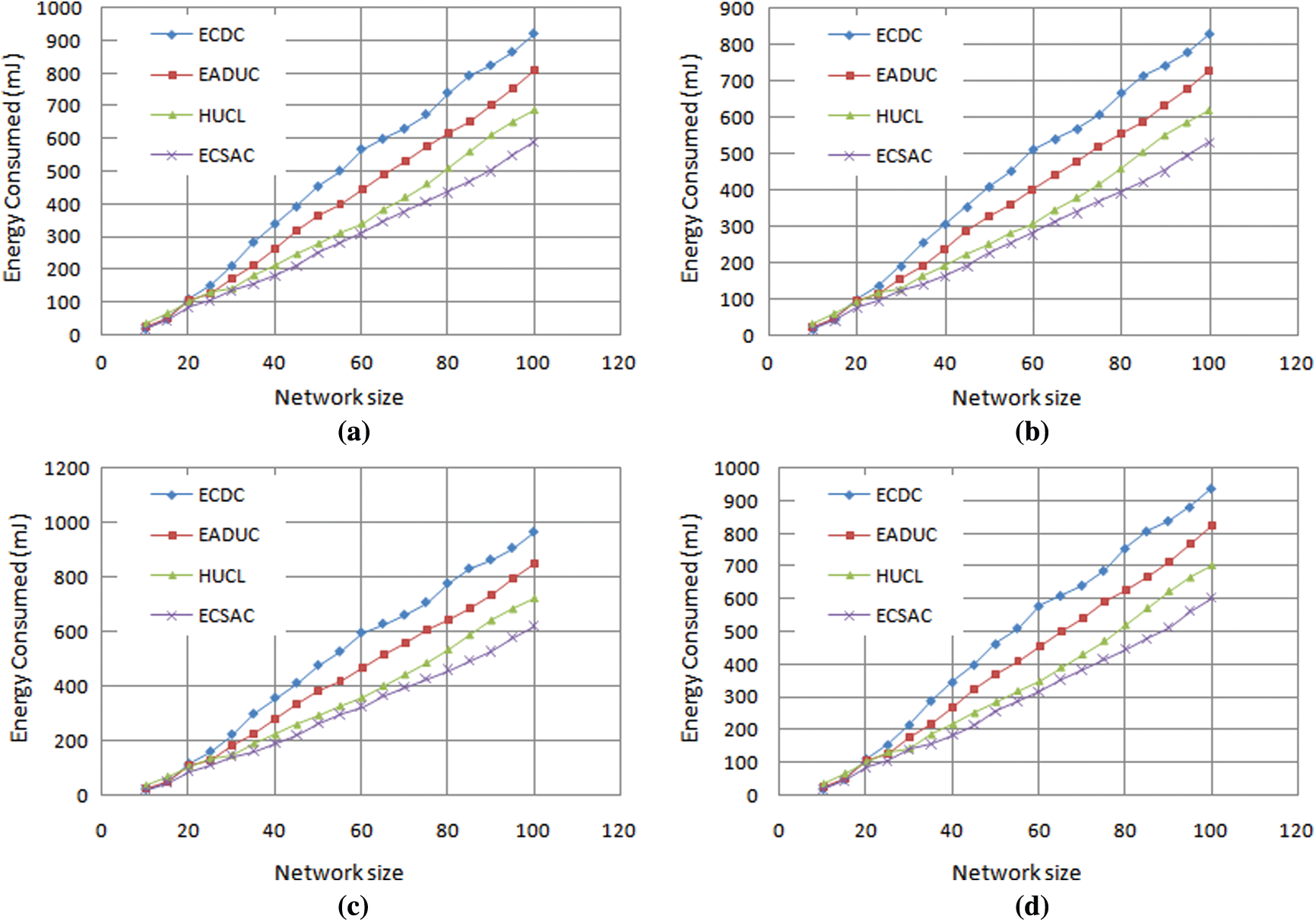
Figure 6: (a) Energy consumption during the transmission phase scenario 1. (b) Energy consumption during the transmission phase Scenario 2. (c) Energy consumption during the transmission phase Scenario 3 (d) Energy consumption during the transmission phase Scenario 4
When it comes to our methodology, the rate at which energy is spent is polynomial. The outcomes also show that the energy spent by CATUB is the least compared to other algorithms as it finds the best method amid various probable methodologies with effective backtracking. Meantime, the job done by HUCL is at par with CATUB considering tiny networks; CATUB outdoes for the more extensive networks, resulting in the prevention of loss of energy and its conservation around 24% in a data collection period. As per the outcomes, we agree that in the suggested methodology, the energy consumption was minimized by minimizing the network overhead.
WSNs come with certain restrictions like energy sources for energy consumption as they are directly connected to the transmission. Fine-tuning energy consumption in routing protocols is an essential process for increasing the lifetime of the network. This work has been expanded to improve the life of the WSN by EADUC. This research also used the non-uniform approach to clustering. Based on unequal competitive ranges, the shaped clusters are of uneven scale. There are smaller clusters nearer to the BS compared to the ones away from the BS. By using several factors, the nodes are assigned an uneven radius of competitiveness. It increases energy spent within the CH nodes. The outcome indicates that ECSAC can efficiently augment the network’s steadiness and lifetime compared to ECDC, HUCL and EADUC.
Funding Statement: The authors received no specific funding for this study.
Conflicts of Interest: The authors declare that they have no conflicts of interest to report regarding the present study.
1. X. Gu, J. Yu, G. Wang and Y. Lv, “ECDC: An energy and coverage-aware distributed clustering protocol for wireless sensor networks,” Computers and Electrical Engineering, vol. 40, no. 2, pp. 384–398, 2014. [Google Scholar]
2. S. V. Purkar and R. S. Deshpande, “Energy-efficient clustering protocol to enhance performance of heterogeneous wireless sensor network: EECPEP-HWSN,” Journal of Computer Networks and Communications, vol. 2018, pp. 12, 2018. [Google Scholar]
3. R. Elhabyan, W. Shi and M. St-Hilaire, “Coverage protocols for wireless sensor networks: Review and future directions,” Journal of Communications and Networks, vol. 21, no. 1, pp. 45–60, 2019. [Google Scholar]
4. P. Ayona and A. Rajesh, “Investigation of energy-efficient sensor node placement in railway systems,” Engineering Science and Technology, an International Journal, vol. 19, no. 2, pp. 754–768, 2016. [Google Scholar]
5. V. Kaundal, A. K. Mondal, P. Sharma and K. Bansal, “Tracing of shading effect on underachieving SPV cell of an SPV grid using wireless sensor network,” Engineering Science and Technology, an International Journal, vol. 18, no. 3, pp. 475–484, 2015. [Google Scholar]
6. A. F. Liu, W. X. You, C. Z. Gang and G. W. Hua, “Research on the energy hole problem based on unequal cluster-radius for wireless sensor networks,” Computer Communications, vol. 33, no. 3, pp. 302–321, 2010. [Google Scholar]
7. T. Liu, J. Peng, Y. Jin, G. Chen and W. Xu, “Avoidance of energy hole problem based on a feedback mechanism for heterogeneous sensor networks,” International Journal of Distributed Sensor Networks, vol. 13, no. 6, pp. 155014771771362, 2017. [Google Scholar]
8. S. H. Kang and T. Nguyen, “Distance-based thresholds for cluster head selection in wireless sensor networks,” IEEE Communications Letters, vol. 16, no. 9, pp. 1396–1399, 2012. [Google Scholar]
9. M. Zeng, X. Huang, B. Zheng and X. Fan, “A heterogeneous energy wireless sensor network clustering protocol,” Journal on Wireless Communications and Mobile Computing, vol. 2019, no. 1, pp. 1–11, 2019. [Google Scholar]
10. N. Vlajic and D. Xia, “Wireless sensor networks: To cluster or not to cluster?,” in Int. Symp. on a World of Wireless, Mobile and Multimedia Networks (WoWMoM’06Buffalo-Niagara Falls, NY, USA, pp. 260–268, 2016. https://doi.org/10.1109/WOWMOM.2006.116. [Google Scholar]
11. M. M. Raouf and J. B. Iraq, “Clustering in wireless sensor networks (WSNs),” Journal of Baghdad University College of Economic Sciences, vol. 57, pp. 01–09, 2019. [Google Scholar]
12. W. B. Heinzelman, A. Chandrakasan and H. Balakrishnan, “Energy-efficient communication protocol for wireless microsensor networks,” in Proc. of the 33rd Annual Hawaii Int. Conf. on System Sciences, Maui, HI, USA, 2, pp. 10, 2000. [Google Scholar]
13. A. F. Jemal, R. H. Hussen, D.-Y. Kim and Z. Li, “Energy-efficient selection of cluster headers in wireless sensor networks,” International Journal of Distributed Sensor Networks, vol. 14, no. 3, pp. 1–9, 2018. [Google Scholar]
14. K. Mahmood Awan, A. Ali, F. Aadil and K. N. Qureshi, “An energy-efficient cluster-based routing algorithm for wireless sensors networks,” in 2018 Int. Conf. on Advancements in Computational Sciences (ICACSLahore, pp. 1–7, 2018. [Google Scholar]
15. O. Younis and S. Fahmy, “HEED: A hybrid, energy-efficient, distributed clustering approach for ad hoc sensor networks,” IEEE Transaction on Mobile Computing, vol. 3, no. 4, pp. 366–379, 2004. [Google Scholar]
16. B. Tavli, “Energy-efficient is relaying in wireless networks,” International Journal of Electronics and Communications, vol. 63, no. 8, pp. 695–698, 2009. [Google Scholar]
17. M. Arifur Rahman, Y. D. Lee and I. Kee, “Energy-efficient power allocation and relay selection schemes for relay-assisted D2D communications in 5G wireless networks,” Sensors (Basel), vol. 18, no. 9, pp. 2865, 2018. [Google Scholar]
18. A. Kozłowski and J. Sosnowski, “Energy efficiency trade-off between duty-cycling and wake-up radio techniques in IoT Networks,” Wireless Personal Communications, vol. 107, no. 4, pp. 1951–1971, 2019. [Google Scholar]
19. R. C. Carrano, D. Passons, L. C. S. Maglhaes and V. N. Albuquerque, “Survey and taxonomy of duty cycling mechanisms in wireless sensor networks,” IEEE Communication Surveys and Tutorials, vol. 16, no. 1, pp. 181–192, 2014. [Google Scholar]
20. J. Lian, K. Naik and G. Agnew, “Data capacity improvement of wireless sensor networks using non-uniform sensor distribution,” International Journal of Distributed Sensor Networks, vol. 2, no. 2, pp. 121–145, 2006. [Google Scholar]
21. X. Wu, G. Chen and S. K. Das, “Avoiding energy holes in wireless sensor networks with non-uniform node distribution,” IEEE Transaction on Parallel and Distributed Systems, vol. 19, no. 5, pp. 710–720, 2008. [Google Scholar]
22. A. Khan, A. Khursheed, E.-U.-H. Qazi and A. Ur Rahman, “Energy-aware scalable reliable and void-hole mitigation routing for sparsely deployed underwater acoustic networks,” Applied Sciences, vol. 10, no. 1, pp. 177, 2020. [Google Scholar]
23. C. Zhu, S. Wu, G. Han, L. Shu and H. Wu, “A tree-cluster based data gathering algorithm for industrial WSNs with a mobile sink,” IEEE Access, vol. 3, pp. 381–396, 2015. [Google Scholar]
24. D. Djenouri and I. Balasingham, “Traffic-differentiation- based modular QoS localized routing for wireless sensor networks,” IEEE Transactions on Mobile Computing, vol. 10, no. 6, pp. 797–809, 2011. [Google Scholar]
25. L. Badia, A. Botta and L. Lenzini, “A genetic approach to joint routing and link scheduling for wireless mesh networks,” International Journal of Ad Hoc Networks, vol. 7, no. 4, pp. 654–664, 2009. [Google Scholar]
26. J. Jia, X. Wang and J. Chen, “A Genetic approach on cross-layer optimization for cognitive radio wireless mesh network under SINR model,” International Journal on Ad Hoc Networks, vol. 27, no. 4, pp. 57–67, 2015. [Google Scholar]
27. A. Amin and G. Miao, “Lifetime-aware scheduling and power control for M2M communications in LTE networks,” in IEEE 81st, IEEE Conf. Proc. Vehicular Technology Conf. (VTC SpringNew Orleans, LA, USA, 2015. [Google Scholar]
28. Y. Gu, M. Pan and W. W. Li, “Prolonging the lifetime of large scale wireless sensor networks via base station placement,” in IEEE 78th Conf. on Vehicular Technology (VTC FallLas Vegas, NV, USA, pp. 1–5, 2013. [Google Scholar]
29. Y. Shi, Y. E. Sagduyuand and J. H. Li, “Low complexity multi-layer optimization for multi-hop wireless networks,” IEEE Conf. on Military Communications, Orlando, FL, USA, pp. 1–6, 2012. [Google Scholar]
30. A. B. M. Alim Al Islam, M. S. Hossain, V. Raghunathan and Y. C. Hu, “Backpacking: Energy-efficient deployment of heterogeneous radios in multi-radio high-data-rate wireless sensor networks,” IEEE Access, vol. 2, pp. 1281–1306, 2014. [Google Scholar]
31. L. Jun, M. Dong, K. Ota and A. Liu, “Achieving source location privacy and network lifetime maximization through tree-based diversionary routing in wireless sensor networks,” IEEE Access, vol. 2, pp. 633–651, 2014. [Google Scholar]
32. J. Yu, Y. Qi and G. Wang, “An energy-driven unequal clustering protocol for heterogeneous wireless sensor networks,” Journal of Control Theory and Applications, vol. 9, no. 1, pp. 133–139, 2011. [Google Scholar]
33. U. Hari, B. Ramachandran and C. Johnson, “An unequally clustered multihop routing protocol for wireless sensor networks,” in Proc. of Int. Conf. on Advances in Computing, Communications, and Informatics, Mysore, India, pp. 1007–1011, 2013. [Google Scholar]
34. M. M. Afsar and M.-H. Tayarani-N, “Clustering in sensor networks: A literature survey,” Journal of Network and Computer Applications, vol. 46, no. 4, pp. 198–226, 2014. [Google Scholar]
35. O. Younis. and S. Fahmy, “HEED: A hybrid, energy-efficient, distributed clustering approach for Ad hoc sensor networks,” IEEE Transactions on Mobile Computing, vol. 3, no. 4, pp. 366–379, 2004. [Google Scholar]
36. Y. Y. Qi, J. G. Yu and N. N. Wang, “An energy-efficient distributed clustering algorithm for wireless sensor networks,” Computer Engineering, vol. 37, no. 1, pp. 83–89, 2011. [Google Scholar]
37. S. Soro and W. B. Heinzelman, “Prolonging the lifetime of wireless sensor networks via unequal clustering,” in Proc. of the 19th IEEE Int. Parallel and Distributed Processing Symp., USA, 2018, pp.236–243,2005. [Google Scholar]
38. C. Li, M. Ye, G. Chen and J. Wu, “An energy-efficient unequal clustering mechanism for wireless sensor networks,” in IEEE Int. Conf. on Mobile Adhoc and Sensor Systems Conf., Washington, DC, USA, 2005. [Google Scholar]
39. A. Naushad, G. Abbas and S. A. Shah, “Energy-efficient clustering with reliable and load-balanced multipath routing for WSNs,” in IEEE Int. Conf. on Advancements in Computational Science, Lahore, Pakistan, 2020. [Google Scholar]
 | This work is licensed under a Creative Commons Attribution 4.0 International License, which permits unrestricted use, distribution, and reproduction in any medium, provided the original work is properly cited. |