Computers, Materials & Continua DOI:10.32604/cmc.2021.015252
Article

The Investigation of the Fractional-View Dynamics of Helmholtz Equations Within Caputo Operator

Rashid Jan1, Hassan Khan2,3, Poom Kumam4,5,*, Fairouz Tchier6, Rasool Shah2 and Haifa Bin Jebreen6

1Department of Mathematics and Statistics, Bacha Khan University, Charsadda, 24420, Pakistan
2Department of Mathematics, Abdul Wali Khan University, Mardan, 23200, Pakistan
3Department of Mathematics, Near East University TRNC, Mersin, 10, Turkey
4Center of Excellence in Theoretical and Computational Science (TACS-CoE) & Department of Mathematics, Faculty of Science, King Mongkut’s University of Technology Thonburi (KMUTT), 126 Pracha-Uthit Road, Bang Mod, Thung Khru, 10140, Bangkok, Thailand
5Department of Medical Research, China Medical University Hospital, China Medical University, Taichung 40402, Taiwan
6Mathematics Department, King Saud University, Riyadh, Saudi Arabia
*Corresponding Author: Poom Kumam. Email: poom.kum@kmutt.ac.th
Received: 12 November 2020; Accepted: 24 December 2020

Abstract: It is eminent that partial differential equations are extensively meaningful in physics, mathematics and engineering. Natural phenomena are formulated with partial differential equations and are solved analytically or numerically to interrogate the system’s dynamical behavior. In the present research, mathematical modeling is extended and the modeling solutions Helmholtz equations are discussed in the fractional view of derivatives. First, the Helmholtz equations are presented in Caputo’s fractional derivative. Then Natural transformation, along with the decomposition method, is used to attain the series form solutions of the suggested problems. For justification of the proposed technique, it is applied to several numerical examples. The graphical representation of the solutions shows that the suggested technique is an accurate and effective technique with a high convergence rate than other methods. The less calculation and higher rate of convergence have confirmed the present technique’s reliability and applicability to solve partial differential equations and their systems in a fractional framework.

Keywords: Fractional-order Helmholtz equations; fractional calculus; {natural} transform decomposition method; analytic solution

1  Introduction

The research area of mathematics interrogating the non-integer properties of derivatives and integrals is called fractional calculus. Fractional calculus has become popular in recent years due to its application in a real-world problem. However, its history is as ancient as ordinary derivative [1,2] and is developed by Leibniz, Liouville, Heaviside, Riemann, Fourier, Lagrange, Abel, Euler [3] etc. Recently, it becomes prevalent and had several real-life applications; moreover, it has been proved that the system developed from natural phenomena can be expressed more accurately through fractional derivative than the ordinary derivative. The applications of fractional calculus occur in control theory, viscoelasticity, electrical networks, diffusive transport akin to diffusion, fluid flow, rheology, optics and signals processing, dynamical processes in the porous structure, probability and statistics, electrochemistry of corrosion and many other branches of economics, physics, engineering and mathematics [4–6].

Hermann Von Helmholtz introduced the concept of the following equation

∇2φ(x,y,z)+χ2φ(x,y,z)=0, (1)

which demonstrates the time-independent structure of diffusion or wave equation achieved during the implementation of the separable variables technique and make the solution procedure much easier. The Helmholtz equation of dimensional two arises in engineering applications and physical phenomena [7–9] such as water wave propagation, acoustic radiation, heat conduction and even in biology. The importance of the fractional derivative cannot be ignored because it estimates the geodesic seafood properties, acoustic propagation in shallow water as well as at low frequencies. Fractional derivatives provide more accurate results and conceptualize different phenomena in a better way in the form of mathematical model [10–17].

It is well known that the problems in pattern formation animal coating [18] in electro-magnetics are also solved through Helmholtz equation, where its two-dimensional structure becomes more applicable in different areas. Several numerical methods have been utilized to solve the above Eq. (1), in which the integral surface method and the Ritz–Galerkin method [19] consume a large unit of time by computing the problem numerically. In contrast, the finite element method [20] produces inaccurate results during computation of the problem. Therefore, we use NTDM to reduce these inaccuracies and to lessen the computational time for our problem. Here, we represent the Helmholtz equations with x and y−space in the following manner

{∂ϑV(x,y)∂xϑ+∂2V(x,y)∂y2+ηV(x,y)=ϕ(x,y),∂ϑV(x,y)∂yϑ+∂2V(x,y)∂x2+ηV(x,y)=ϕ(x,y), (2)

with proper initial conditions given by

V(0,y)=φy, and V(x,0)=φx,

where ϑ is the fractional-order which lesson the memory requirements. In the above (2) both x and y have the choices to change the fractional order.

The Natural transform decomposition method is developed by using the two powerful methods that are Adomian decomposition and Natural transform, which solve many PDEs and FPDEs arises from physical phenomena. Specifically, numerous non-linear PDEs [21,22], non-linear ODEs [23] and fractional-order models and equations [24–26] are solved by NTDM. It has been shown that the convergence rate of the NTDM are higher than MHPM and HPM and are more accurate than the MHPM and HPM.

In the present article, NTDM is implemented in a very simple and sophesticated manner to analyse the solutions of fractional-order Helmholtz equations. Three numerical examples were considered for analytical treatment. The successful NTDM schemes or algorithms are derived for both fractional and integer orders of the problems. First, the natural transformation is applied to reduce the given problems into simpler forms and then Adomian decomposition method is used to investigate the final solutions of the problems. The derived results are then plotted and have shown that the present solutions are in best contact with the solutions of LADM [16] and FRDTM [17]. The fractional solutions graphs are plotted and the convergence phenomenan of fractional-orders solutions towards integer-order solutions is observed. Beside these it is also analysed that NTDM is very simple and straightforward with no need of discritization and required very less computational work. In the view of the above novelty, the present work can be extended to solve other nonlinear FPDEs and their systems.

The article is structured as: The fractional-order Helmholtz equations are represented with x-space and y-space in Section 1. In Section 2 of the article, we present the elementary theory of fractional calculus and Natural Transform Decomposition Method. The general idea of the NTDM is introduced and applied to the proposed fractional Helmholtz equations in Section 3. In Section 4, the proposed concept of the NTDM is applied to several numerical examples to understand the procedure of the proposed method; moreover, numerous numerical simulations are used to show the graphical results of the fractional-order problem. Finally, the overall conclusion of the article is presented in Section 5.

2  Rudimentary Theory

In this section of the article, we represent Caputo’s fractional operator to inspect our proposed problem. In addition to this, we will give the basic concept of natural transform, inverse natural transform and the natural transform of n-th derivative for further analysis and investigation.

2.1 Definition [3,27]

Assume a function h in a manner that h∈Ct1 then the fractional derivative of h through Caputo’s operator of order ϑ is given by

Dϑh(x)=∂ϑh(x)∂t1ϑ=In−ϑ(∂ϑh(x)∂t1ϑ), if n−1<ϑ≤n, n∈N=∂ϑh(x)∂t1ϑ. (3)

where n∈N, x>0, t1≥−1.

2.2 Definition [3,27]

Let ϑ>0 and q∈C then the Mittag-Leffler function is symbolized by Eϑ(q) and is given by the below-mentioned series

Eϑ(q)=∑n=0∞qnΓ(ϑn+1),ϑ>0.

2.3 Definition [28,29]

For a given function h, the natural transform is given by

N+[h(t1)]=Q(s,v)=1v∫0∞e−st1vh(t1)dt1,

in which s and v indicate the transform variables and are positive.

2.4 Definition [28,29]

For a given function h, the inverse natural transform is given by the following mentioned definition

N−[Q(s,v)]=h(t1)=12πi∫p−i∞p+i∞est1vQ(s,v)ds,

in which p is a real number, s and vindicates Natural transform variables, and the integral in the plane s=x+iy is taken along s=p.

2.5 Definition [28,29]

Let h be a function then the natural transform of n-th derivative is defined by the following manner

N[hn(t1)]=Qn(s,v)=snvnQ(s,v)−∑k=0n−1sn−(k+1)vn−khk(0),

where n≥1 in this definition.

2.6 Theorem [28,29]

Let the transform functions of H(s,u) and L(s,u) are given by h(t1) and l(t1), then we have the following

N[h∗l]=uH(s,u)L(s,u),

where the convolution of the h mentioned above and l is indicated by h∗l.

2.7 Definition [28,29]

Let h be a given function then R-L fractional integral is given as

Ixϑh(x)=h(x) if ϑ=01Γ(ϑ)∫0x(x−v)ϑ−1h(v)dv if ϑ>0,

in which Γ indicates the gamma function, and is given by

Γ(ϖ)=∫0∞e−xxϖ−1dx ϖ∈C.

In the next section of the article, we will give a general concept of fractional NTDM for the solution of Helmholtz equations.

3  Conceptualization of Fractional NTDM [21,22]

Here, we will study the standard concept and procedure of fractional Natural transform decomposition method to solve Helmholtz equations. First, we take the Helmholtz equation in fractional framework with x-space as

∂ϑV(x,y)∂xϑ+∂2V(x,y)∂y2+κV(x,y)=ϕ(x,y), (4)

with the following suitable initial condition

V(0,y)=φy,

and y-space

∂ϑV(x,y)∂yϑ+∂2V(x,y)∂x2+κV(x,y)=ϕ(x,y), (5)

with the below mentioned initial condition

V(x,0)=φx.

Utilizing the Natural transform decomposition method to (4), we have

N+(∂ϑV(x,y)∂xϑ)+N+(∂2V(x,y)∂y2+κV(x,y))=N+[ϕ(x,y)],

and applying the differentiation property of Natural transform decomposition, the following is obtained

N+[V(x,y)]=V(0,y))s+vϑsϑN+[ϕ(x,y)]−vϑsϑN+(∂2V(x,y)∂y2+κV(x,y)). (6)

After that, the Natural transform decomposition method solution V(x,y) is given by the below-mentioned series

V(x,y)=∑j=0∞Vj,

moreover, the following series of Adomian polynomials define the nonlinear term of the problem

N(V(x,y))=∑j=0∞Dj,

Dj=1j!(djdλj(N∑j=0∞(λjvj)))λ=0,

using Natural transform decomposition method solution in (6), the following is obtained

N+[V(x,y)]=V(0,y)s+vϑsϑN+(ϕ(x,y)]−vϑsϑN+(∂2∂y2∑j=0∞Vj+κ∑j=0∞Vj).

Using the linearity of the Natural transform, we have

N+[V0(x,y)]=V(0,y)s+vϑsϑN+[ϕ(x,y)],

N+[∑j=1∞Vj]=−vϑsϑN+(∂2∂y2∑j=0∞Vj+η∑j=0∞Vj).

Now, utilizing the inverse of Natural transform, we can compute Vj (j≥0).

V0(x,y)=V(0,y)+N−(vϑsϑN+[ϕ(x,y))),

∑j=1∞Vj=−N−(−vϑsϑN+(∂2∂y2∑j=0∞Vj+η∑j=0∞Vj)).

4  Applications and Numerical Simulations

In this section of the article, the method NTDM will be applied to some examples to understand the procedure of the proposed method. In the end, some numerical simulations are carried out to visualize family of Helmholtz equations through Natural transform decomposition method.

Example 1

Let us take the Helmholtz equation in fractional framework with x-space in the following form [30,31]

∂ϑV(x,y)∂xϑ+∂2V(x,y)∂y2−V(x,y)=0,1<ϑ≤2 (7)

with the below mentioned initial value

V(0,y)=y. (8)

First of all, take the Natural transform of (7), we obtain the following

N+(∂ϑV(x,y)∂xϑ)=N+(V(x,y)−∂2V(x,y)∂y2),

sϑvϑN+(V(x,y))−sϑ−1vϑV(0,y)=N+(V(x,y)−∂2V(x,y)∂y2).

In the next step, we use the Natural inverse transform and get

V(x,y)=N−1(V(0,y)s+vϑsϑN+(V(x,y)−∂2V(x,y)∂y2)).

Then, applying the procedure of NTDM, the following is obtained

V0(x,y)=N−1(V(0,y)s)=N−1(ys) (9)

Vj+1=N−1(vϑsϑN+(Vj−∂2∂y2Vj)),j=0,1,2,….

For j=0, we have

V1=N−1(vϑsϑN+(V0−∂2∂y2V0)),V1(x,y)=N−1(yvϑsϑ+1)=yxϑΓ(ϑ+1). (10)

The subsequent terms are

V2(x,y)=N−1(vϑsϑN+(V1−∂2∂y2V1))=yx2ϑΓ(2ϑ+1),V3(x,y)=N−1(vϑsϑN+(V2−∂2∂y2V2))=yx3ϑΓ(3ϑ+1),V4(x,y)=N−1(vϑsϑN+(V3−∂2∂y2V3))=yx4ϑΓ(4ϑ+1),....Vj+1=N−1(vϑsϑN+(Vj−∂2∂y2Vj))=yxjϑΓ(jϑ+1). (11)

Thus the solution of (4) through NTDM is

V(x,y)=V0(x,y)+V1(x,y)+V2(x,y)+V3(x,y)+V4(x,y)+…

V(x,y)=y(1+xϑΓ(ϑ+1)+x2ϑΓ(2ϑ+1)+x3ϑΓ(3ϑ+1)+x4ϑΓ(4ϑ+1)+…),

in the case when ϑ=2, then the solution of the problem through NTDM is

V(x,y)=ycosh⁡x.

In the same way, the solution of y-space can be determined through NTDM as:

∂ϑV(x,y)∂yϑ+∂2V(x,y)∂x2−V(x,y)=0, (12)

with the proper initial value

V(x,0)=x. (13)

Thus the solution of the above (12) is given by

V(x,y)=x(1+yϑΓ(ϑ+1)+y2ϑΓ(2ϑ+1)+y3ϑΓ(3ϑ+1)+y4ϑΓ(4ϑ+1)+…),

in the case when ϑ=2, then the solution through NTDM is

V(x,y)=xcosh⁡y. (14)

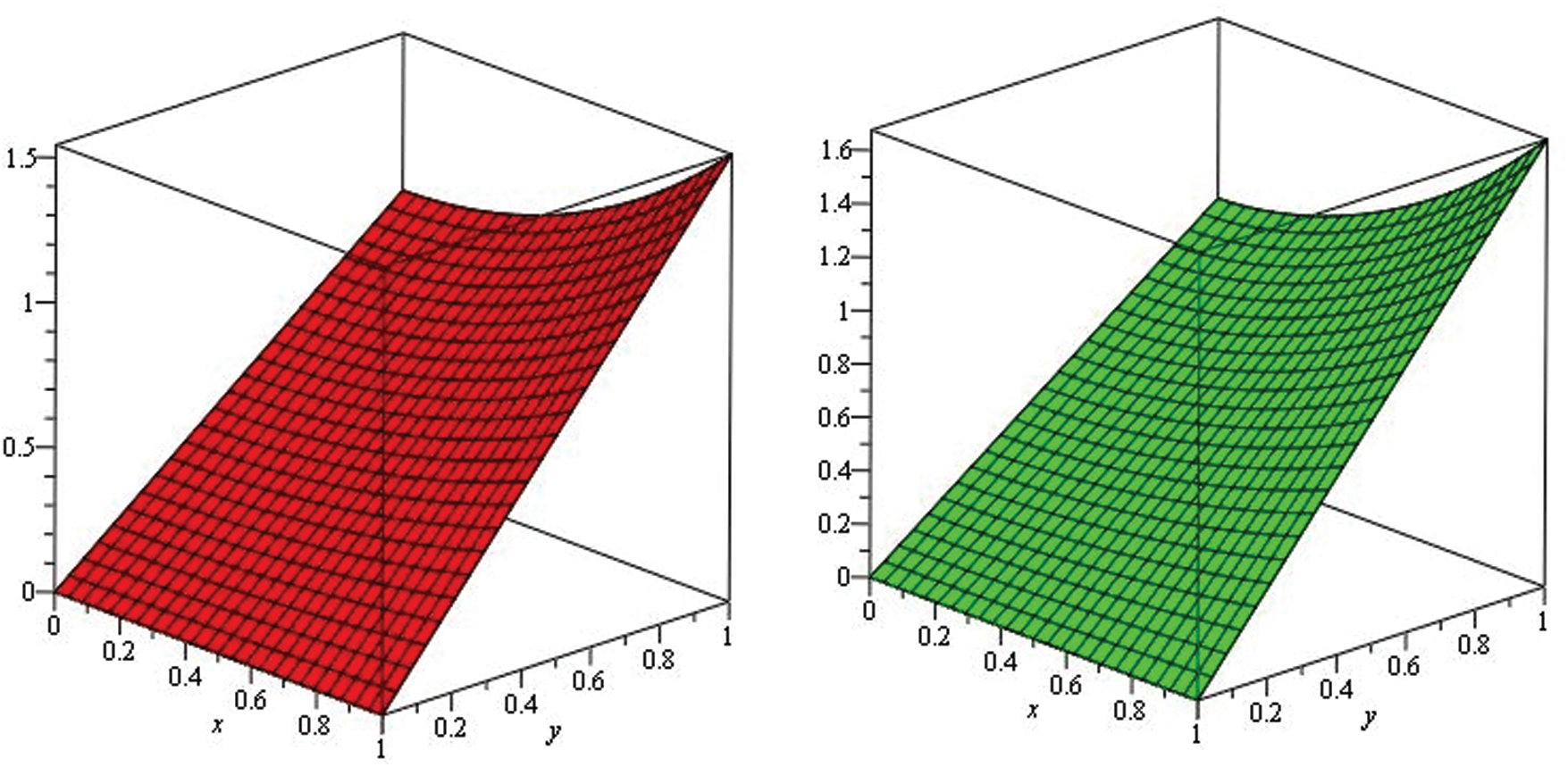
Figure 1: Illustration of solution pathways: (Left) The red figure represent the solution of Example 1 through NTDM for fractional-order ϑ=1 and (Right) The green figure represent the solution of Example 1 through NTDM for fractional-order ϑ=0.8

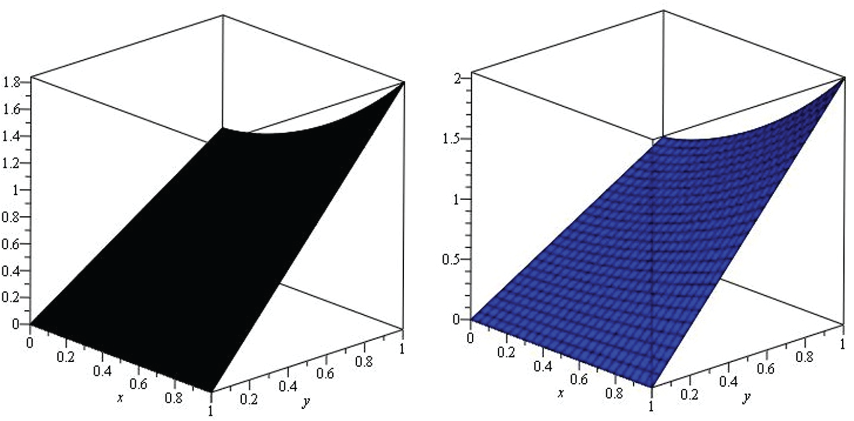
Figure 2: Illustration of solution pathways: (Left) The black figure represent the solution of Example 1 through NTDM for fractional-order ϑ=0.6 and (Right) The blue figure represents the solution of Example 1 through NTDM for fractional-order ϑ=0.4

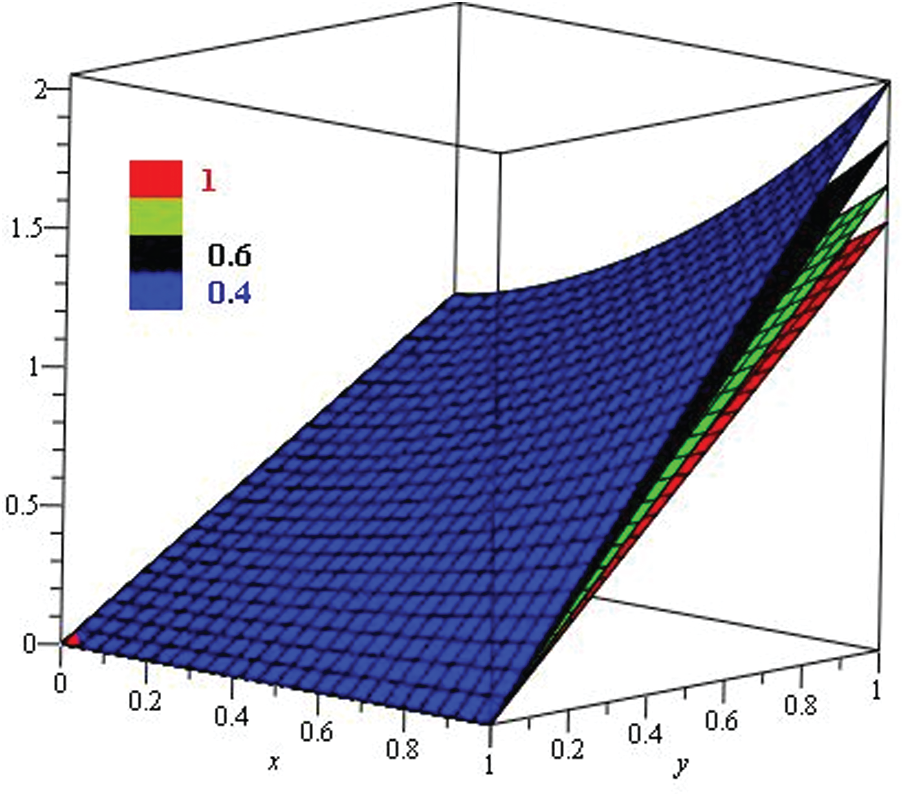
Figure 3: The solution v(x,y,t1) of our proposed Example 1 through the proposed NTDM with varies values of fractional order ϑ

Example 2

Let us take homogeneous Helmholtz equation in fractional framework with x-space and η=5 as follows [30,31]

∂ϑV(x,y)∂xϑ+∂2V(x,y)∂y2+5v(x,y)=0,1<ϑ≤2 (15)

with initial values given by

V(0,y)=y. (16)

Here, taking the natural transform of (15), we have

N+(∂ϑV(x,y)∂xϑ)=−N+(5V(x,y)+∂2V(x,y)∂y2),

sϑvϑN+(V(x,y)−sϑ−1vϑV(0,y))=−N+(5V(x,y)+∂2V(x,y)∂y2).

After that, we apply inverse Nature transform to our problem and get

V(x,y)=N−1(V(0,y)s−vϑsϑN+(5V(x,y)+∂2V(x,y)∂y2)),

Applying the ADM procedure, we have the following

V0(x,y)=N−1(V0(0,y)s)=N−1(ys),

Vj+1=N−1(−vϑsϑN+(∂2∂y2Vj+5Vj]),

for j=0,1,2,…. In the case when j=0, we have

V1(x,y)=N−1(−vϑsϑN+(∂2∂y2V0+5V0)),V1(x,y)=N−1(−5yvϑsϑ+1)=−5yxϑΓ(ϑ+1),V2(x,y)=N−1(−vϑsϑN+(∂2∂y2V1+5V1))=25yx2ϑΓ(2+1),V3(x,y)=N−1[−uβsβN+[∂2∂y2U2+5U2]]=−125yx3βΓ(3β+1),V4(x,y)=N−1[−uβsβN+[∂2∂y2U3+5U3]]=625yx4βΓ(4β+1),..Vj+1=N−1(−vϑsϑN+(∂2∂y2Vj+5Vj))=(−5)jyxjϑΓ(jϑ+1). (17)

The solution of the above problem (15) through NTDM is given by

V(x,y)=V0(x,y)+V1(x,y)+V2(x,y)+V3(x,y)+V4(x,y)+…

V(x,y)=y(1−5xϑΓ(ϑ+1)+25x2ϑΓ(2ϑ+1)−125x3ϑΓ(3ϑ+1)+625x4ϑΓ(4ϑ+1)+…),

in the case when ϑ=2, then the solution through NTDM is given by

V(x,y)=ycos⁡5x.

In the same way, we apply NTDM to y-space

∂ϑV(x,y)∂yϑ+∂2V(x,y)∂x2+5V(x,y)=0, (18)

with the initial value given by

V(x,0)=x.

having the following solution (18) through NTDM is

V(x,y)=x(1−5yϑΓ(ϑ+1)+25y2ϑΓ(2ϑ+1)−125y3ϑΓ(3ϑ+1)+625y4ϑΓ(4ϑ+1)+…],

in the case when ϑ=2, the NTDM solution is given by

V(x,y)=xcos⁡5y. (19)

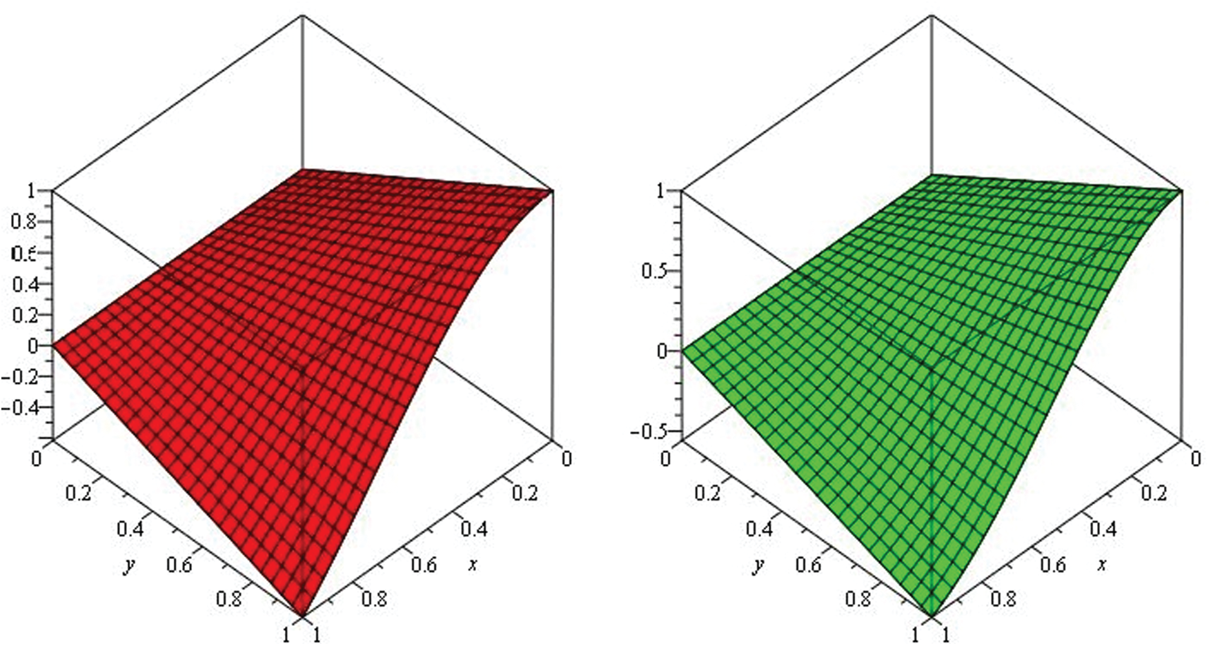
Figure 4: Illustration of solution pathways: (Left) The red figure represent the solution of Example 2 through NTDM for fractional-order ϑ=1 and (Right) The green figure represents the solution of Example 2 through NTDM for fractional-order ϑ=0.8

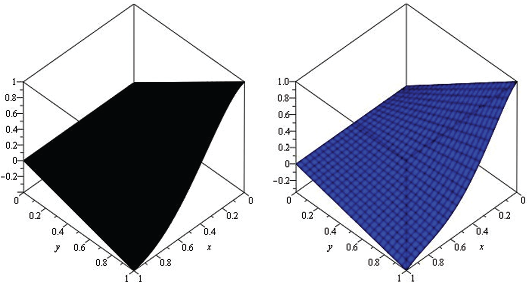
Figure 5: Illustration of solution pathways: (Left) The black figure represent the solution of Example 2 through NTDM for fractional-order ϑ=0.6 and (Right) The blue figure represent the solution of Example 2 through NTDM for fractional-order ϑ=0.4

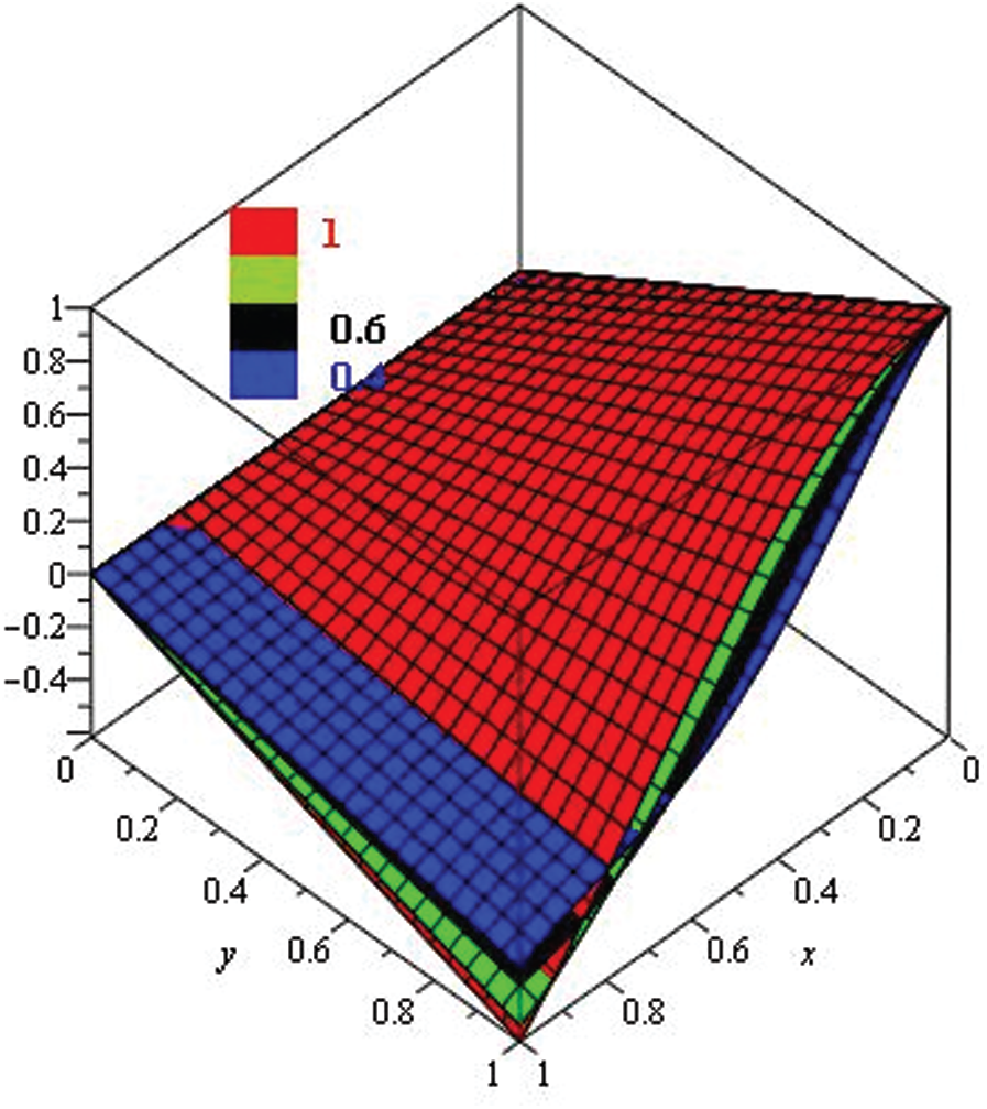
Figure 6: The solution v(x,y,t) of our proposed Example 1 through the proposed NTDM with varies values of fractional order ϑ

Example 3

Assume the Helmholtz equation with x-space and η=−2 in the fractional framework [30,31]

∂ϑV(x,y)∂xϑ+∂2V(x,y)∂y2−2v(x,y)=(12x2−3x4)sin⁡y,0≤y≤2π and 1<ϑ≤2, (20)

with initial value given by

V(0,y)=0, and Vx(0,y)=0. (21)

First of all, take the Nature transform of the above mentioned (20), we have the following

N+(∂ϑV(x,y)∂xϑ)=N+((12x2−3x4)sin⁡y)−N+(∂2V(x,y)∂y2−2V(x,y)).

Then, the NTDM leads to the below mention

V0(x,y)=N−1((24s5−72s7)sin⁡y)=(x4−x610)sin⁡y, (22)

Vj+1=N−1(−vϑsϑN+(∂2∂y2Vj−2Vj)),j=0,1,2…

then, we have the following

V1(x,y)=N−1[−vϑsϑN+[∂2∂y2V0−2V0]],V1(x,y)=N−1[(72sϑ+5−216sϑ+7)sin⁡y]=(72xϑ+4Γ(ϑ+5)−216xϑ+6Γ(ϑ+7))sin⁡y,V2(x,y)=N−1[−vϑsϑN+[∂2∂y2V1−2V1]]=(216x2ϑ+4Γ(2ϑ+5)−648x2ϑ+6Γ(2ϑ+7))sin⁡y,V3(x,y)=N−1[−vϑsϑN+[∂2∂y2V2−2V2]]=(648x3ϑ+4Γ(3ϑ+5)−1944x3ϑ+6Γ(3ϑ+7))sin⁡y,V4(x,y)=N−1[−vϑsϑN+[∂2∂y2V3−2V3]]=(1944x4ϑ+4Γ(4ϑ+5)−5832x2ϑ+6Γ(2ϑ+7))sin⁡y, (23)

The NTDM solution of Example (3.3)

V(x,y)=V0(x,y)+V1(x,y)+V2(x,y)+V3(x,y)+V4(x,y)+…

V(x,y)=(x4−x610)sin⁡y+(72xϑ+4Γ(ϑ+5)sin⁡y−216xϑ+6Γ(ϑ+7))sin⁡y+(216x2ϑ+4Γ(2ϑ+5)−648x2ϑ+6Γ(2ϑ+7))sin⁡y+(648x3ϑ+4Γ(3ϑ+5)−1944x3ϑ+6Γ(3ϑ+7))sin⁡y+(1944x4ϑ+4Γ(4ϑ+5)−5832x2ϑ+6Γ(2ϑ+7))sin⁡y+…, (24)

when ϑ=2, then NTDM solution is

U(x,y)=x4sin⁡y. (25)

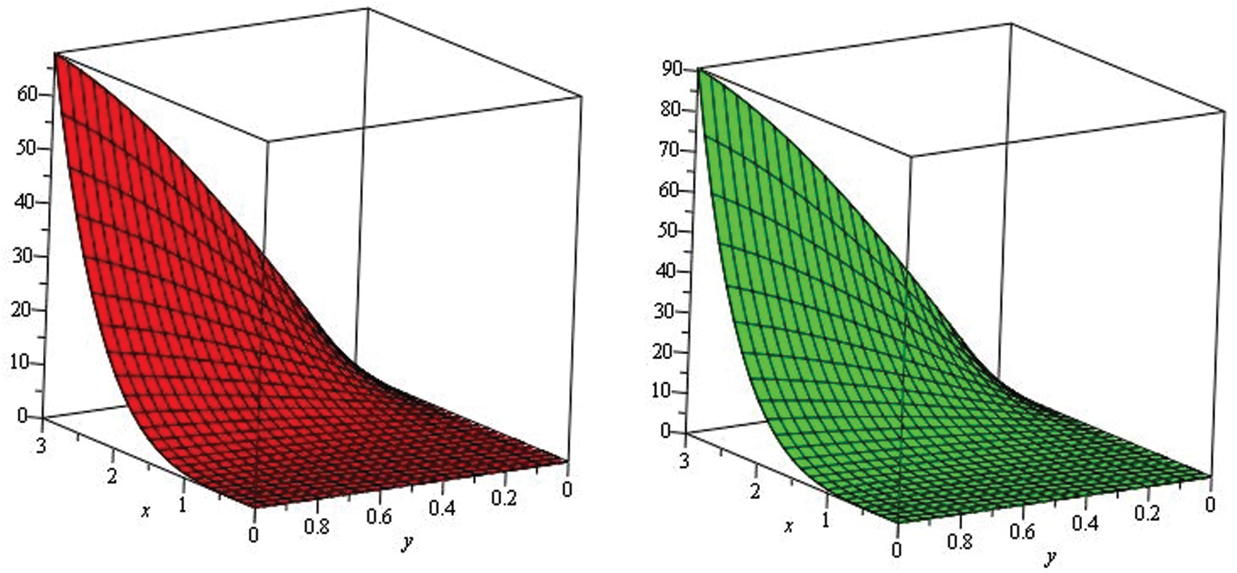
Figure 7: Illustration of solution pathways: (Left) The red figure represent the solution of Example 3 through NTDM for fractional-order ϑ=1 and (Right) The green figure represent the solution of Example 3 through NTDM for fractional-order ϑ=0.8

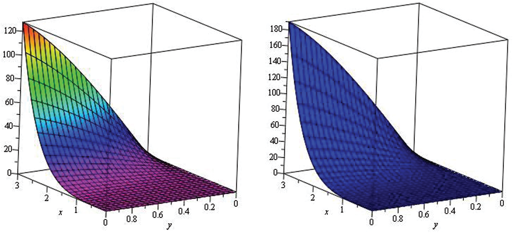
Figure 8: Illustration of solution pathways: (Left) The first figure represent the solution of Example 3 through NTDM for fractional-order ϑ=0.6 and (Right) The second figure represents the solution of Example 3 through NTDM for fractional-order ϑ=0.4

5  Results Discussion

Fig. 1, represents the solution-graphs of example 1 at fractional-orders δ=1 and 0.8, which are represented by left and right sub-graphs of Fig. 1, respectively. Fig. 2 is plotted to show the fractional-order solutions of example 1 at fractional-orders δ=0.6 and 0.4 by the left and right sub-graphs, respectively. In Fig. 3, the combined graph of fractional-order solutions of example 1 is presented and confirmed various dynamical behaviours of the physical phenomenon, which is modelled by the equation given in example 1. In Fig. 4, two subgraphs left and right represented the solution of example 2 at fractional-order ϑ=1 and 0.8, respectively. In Fig. 5, the solutions of example 2 at fractional-order δ=0.6 and 0.4 are discussed. In Fig. 6, the combined graph of fractional-orders solutions at δ=1, 0.8, 0.6 and 0.4 is displaced and the systematic behaviour of the solution is observed. Similarly, in Figs. 6 and 7, the fractional solutions of example 3 are presented at 1, 0.8 and ϑ=0.6, 0.4 respectively. Also, the combined graph, Fig. 8, represent the solution of example 3 at ϑ=1, 0.8, 0.6 and 0.4 collectively. Moreover, in Fig. 9, the combined graphs of fractional-order solutions are represented by two subgraphs, given in Fig. 9 in two and three-dimensional graphs. In both cases, we observed the correct behaviour of the solutions, which confirmed the validity of the suggested method.

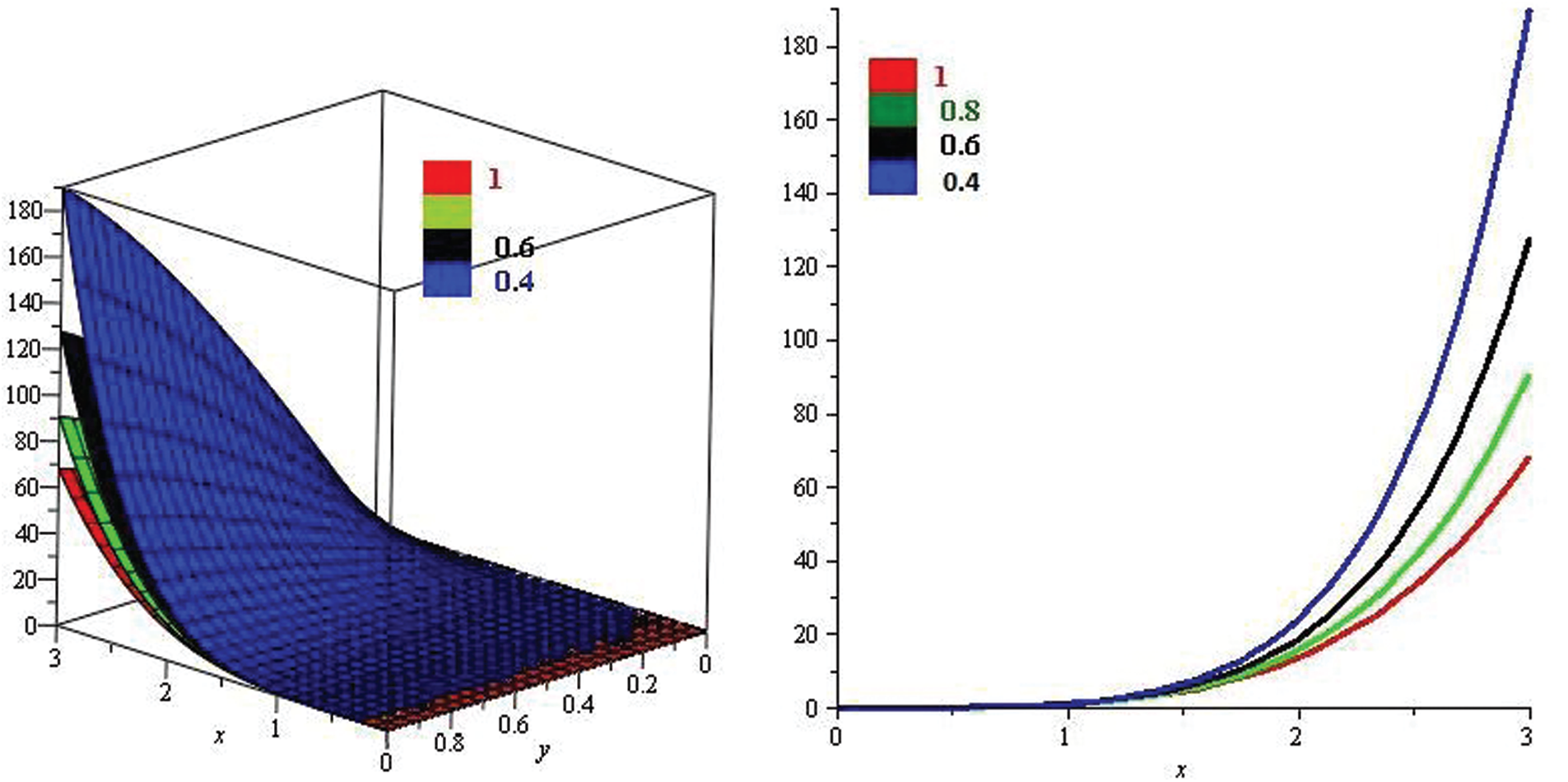
Figure 9: Illustration of the solution of Example 3 through NTDM with varies values of fractional order ϑ

6  Conclusion

In this paper, a new combination of the Adomian decomposition method with Natural transformation is made to find the analytical solutions of fractional-order partial differential equations. It is of worth interest that the implementation of the present technique is very straightforward for the solutions Helmholtz equations in its Caputo fractional-view analysis. Three numerical examples were considered for its analytical solutions by using the proposed techniques. The corresponding solutions-graphs are plotted for both fractional and integer order of the problems. The solutions revealed that the suggested method is very commited and in strong agreement with the solutions of other existing techniques. It is noted that NTDM is an easily computable, precious, accurate technique with a high rate of convergence than the other analytical methods. It is suggested that Natural transform decomposition method is the most reliable technique for solving partial differential equations in fractional framework, specifically, for fractional-order Helmholtz family of equations. The solutions of the fractional-order PDEs through NTDM are more accurate and less time consuming as compare to the ADM, VIM and DTM.

Funding Statement: Center of Excellence in Theoretical and Computational Science (TaCS-CoE) & Department of Mathematics, Faculty of Science, King Mongkut's University of Technology Thonburi (KMUTT), 126 Pracha Uthit Rd., Bang Mod, Thung Khru, Bangkok 10140, Thailand.

Conflicts of Interest: The authors declare that they have no conflicts of interest to report regarding the present study.

This work is licensed under a Creative Commons Attribution 4.0 International License, which permits unrestricted use, distribution, and reproduction in any medium, provided the original work is properly cited.