Computers, Materials & Continua DOI:10.32604/cmc.2021.015441
Article

Modelling Intelligent Driving Behaviour Using Machine Learning

Qura-Tul-Ain Khan1, Sagheer Abbas1, Muhammad Adnan Khan*,2, Areej Fatima3, Saad Alanazi4 and Nouh Sabri Elmitwally4,5

1School of Computer Science, NCBA&E, Lahore, 54000, Pakistan
2Riphah School of Computing & Innovation, Faculty of Computing, Riphah International University, Lahore Campus, Lahore, 54000, Pakistan
3Department of Computer Science, Lahore Garrison University, Lahore, 54000, Pakistan
4Department of Computer Science, College of Computer and Information Sciences, Jouf University, Skaka, Aljouf, 72341, Saudi Arabia
5Department of Computer Science, Faculty of Computers and Artificial Intelligence, Cairo University, 12613, Egypt
*Corresponding Author: Muhammad Adnan Khan. Email: adnan.khan@riphah.edu.pk
Received: 21 November 2020; Accepted: 04 March 2021

Abstract: In vehicular systems, driving is considered to be the most complex task, involving many aspects of external sensory skills as well as cognitive intelligence. External skills include the estimation of distance and speed, time perception, visual and auditory perception, attention, the capability to drive safely and action-reaction time. Cognitive intelligence works as an internal mechanism that manages and holds the overall driver’s intelligent system.These cognitive capacities constitute the frontiers for generating adaptive behaviour for dynamic environments. The parameters for understanding intelligent behaviour are knowledge, reasoning, decision making, habit and cognitive skill. Modelling intelligent behaviour reveals that many of these parameters operate simultaneously to enable drivers to react to current situations. Environmental changes prompt the parameter values to change, a process which continues unless and until all processes are completed. This paper model intelligent behaviour by using a ‘driver behaviour model’ to obtain accurate intelligent driving behaviour patterns. This model works on layering patterns in which hierarchy and coherence are maintained to transfer the data with accuracy from one module to another. These patterns constitute the outcome of different modules that collaborate to generate appropriate values. In this case, accurate patterns were acquired using ANN static and dynamic non-linear autoregressive approach was used and for further accuracy validation, time-series dynamic backpropagation artificial neural network, multilayer perceptron and random sub-space on real-world data were also applied.

Keywords: Machine learning; artificial neural network; ann; time series; intelligent behaviour; agent

1  Introduction

Human error is the main cause of driving problems. Accordingly, driver behaviour modelling has emerged to improve the driving experience by predicting environmental factors, driver intent, and driver and vehicle state. Sensory information and other predictors can helpfully warn the driver of potential dangers. Meanwhile, vehicle behaviour can determine driver state, measuring elements including driving competence and attention level [1]. Understanding a driver’s cognitive load is critical. Autonomous systems can help to automatically identify driver cognitive workload, enabling the development of robust evaluation tools. Driver performance and physiological data can be assessed and measurements collected in real-time. A classification system can detect cognitive load, with physiological data allowing greater classification accuracy [2]. In vehicular systems, drivers usually demonstrate different driving styles. To analyse explicit links between a driver’s dynamic demand and driving style, driving style can be classified as low, moderate and high. This involves recognising driving style according to the vehicle, driving route, design task and driver selection [3].

All aspects of a human’s life are defined by their routine behaviour [4]. Routine describes deliberate behaviour constituting goal-oriented actions performed in different situations [5], actions that are acquired, learned and developed through repeated practice [6]. Good routines enable efficient completion of frequently repeated tasks through predictable behaviours. Variations in routine behaviour importantly indicate human response because behaviour is not static [7].

Current research is directed towards finding driver behaviour solutions that can avoid road safety problems, especially by identifying and understanding the relationship between road safety and driver behaviour. The major contributing factors to traffic accidents are weather, traffic, vehicle control, and driver sensitivity to complex environments. However, traffic accidents are ultimately largely dependent on the rational judgement and decision making of drivers [8].

Behaviour analysis involves two different approaches to understanding decision-making: analysing the beliefs and the values behind the process and evaluating decision-making according to personality traits and individual habits. This method is quantifiable and can be represented in applications of classifying drivers based on their driving style [9].

2  Literature Review

Thinking essential to understanding the world and managing different situations, problems and relationships [10]. To encourage environmentally responsive behaviour, researchers have used people-oriented approaches which reduce feelings of helplessness and provide sources for motivations [11]. Such approaches allow people to accomplish repetitive tasks at different levels using the human routines that are the blueprints of behaviour. Human routines are expressed through actions performed in particular situations, with behaviour modelling enabling people to improve their inexpert behaviour and change bad habits [4].

Driving output is determined by various factors, with drivers considered the most unstable factors because they exhibit different driving styles. Driving style constitutes the habitual long-term behaviour of drivers, contributing to the real-time adjustments they make to environmental information [3]. Driver behaviour variables require analysis to represent concepts related to driving habits. Defining driver behaviour as one of several different driving behaviours enables identification of behavioural trends and allows accurate measurement of driving style, with the main goal of driver style classification being to detect behaviour, recognise different techniques and enable learning [12]. For example, some researchers have classified eco-driving according to three categories: trajectory planning, route planning and driver behaviour improvement [13].

Elsewhere, driving styles have been categorised as normal, safe, inattentive and aggressive [9]. Risky speeding is a behavioural pattern pertaining to an aggressive driving style, describing irregular, abrupt or instantaneous changes in vehicle speed, improper vehicle positioning and inconsistent acceleration or braking [14]. Aggressive driving behaviour increases the collision risk and can arise from driver annoyance or attempts to minimise travel time [15]. Although repeated behaviour in a stable context can promote automatic habits which are resistant to change through information-based techniques, such behaviours are context-dependent, meaning a change in context can weaken the habit’s strength and facilitate reflection on that behaviour [16].

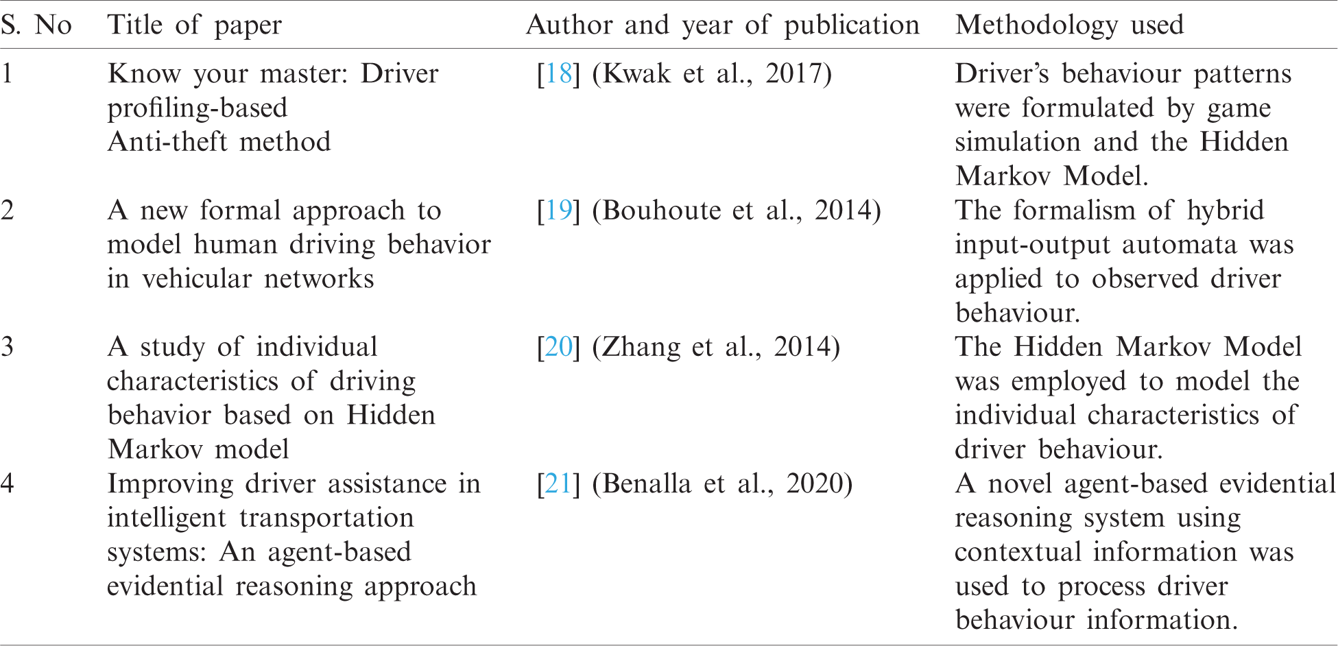
Tab. 1 presents studies on the effects of emotional, sensorimotor, cognitive and mixed stressors on driver behaviour and performance. Notably, another study recognised the effective copying mechanism could reduce behavioural errors caused by cognitive or emotional conflict [17].

Table 1: Comparison of previous work

3  Methodology

The methodology comprised multiple modules (see Fig. 1 for a visual representation): a data acquisition and classification module, a driver ride profiling module, a decision-making module, a memory management module, a route planning module, an assistance system module and an Artificial neural network (ANN) module. Dataset validation involved a dynamic nonlinear autoregressive approach.

3.1 Data Acquisition and Classification

Data acquisition and classification involves collecting environmental, vehicle and cognitive data. Environmental data include weather condition and time of day. Vehicle data include the condition of the vehicle, utilising inputs collected from all parts of the vehicle, including accelerator pressure, braking, steering wheel movement, gear changes and vehicle turns. Cognitive inputs consider parameters such as intentions, motivations, emotions, knowledge, learning and decision-making. This research only analysed environmental and vehicle data.

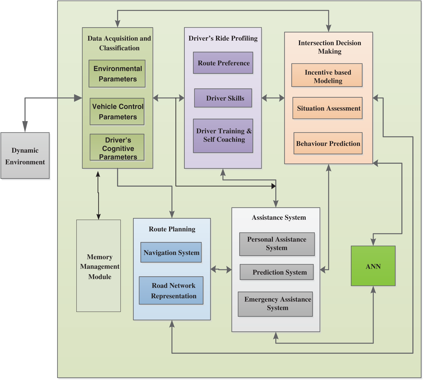
Figure 1: Proposed driver behaviour model

3.2 Driver Ride Profiling

Driver ride profiling includes route preferences, driver skill, driver training and self-coaching. Route preferences includes long, medium and short routes, as well as factors such as terrain. Driver skill refers to driver expertise for a specific route. Driver training and self-coaching incorporate iterative learning, which describes driving training for a specific route.

3.3 Decision-Making Module

The decision-making module incorporates incentive-based modelling, situation assessment and behaviour prediction. Incentive-based modelling is responsible for decisions utilising working progress, which includes the driver’s past experience and how a driver operates a vehicle in a particular scenario, with scenario describing speed and weather condition.

Situation assessment considers the current environment using inputs from the data acquisition and classification, route planning and driver ride profiling modules. The behaviour prediction sub-module predicts behaviour after each complete iteration. Behaviour prediction interacts with the assistance system module to derive data patterns from that module’s personal assistance and prediction systems.

3.4 Memory Management

Memory management stores relevant data and provides requested data to different modules.

3.5 Route Planning

Route planning considers speed limits, road types, traffic jams and weather conditions. Its navigation system includes online maps, available paths and alternative paths, with road network representation used to calculate the path according to road and location conditions.

3.6 Assistance System

The assistance system comprises the personal assistance system, prediction system and emergency assistance system. The personal assistance system guides the driver along their selected route, suggests changes to vehicle speed and assesses driver behaviour. The prediction system helps the driver to predict the next best route, the time of arrival at the destination and the driver’s behaviour in particular scenarios. The emergency assistance system is only activated in case of emergencies, including sudden severe changes in the situation or the driver’s behaviour.

3.7 Driver Behaviour Model Empowered by an Artificial Neural Network

The driver behaviour model uses an ANN to enable smooth data flow and dynamic and intelligent driver behaviour. The ANN is divided into static techniques and dynamic techniques. A dynamic nonlinear autoregressive approach was used to validate the model because driver behaviour is a constantly changing phenomenon. Other validation techniques used were multilayer perceptron and random subspace.

The ANN applied recognised human activity using an artificial backpropagation neural network and featured three layers: an input, output and hidden layer. Every neuron of the hidden layer used the Sigmoid(x) activation function. The proposed ANN is represented mathematically as:

ηΛ=Y1+∑m=1l(tmΛ*jm) (1)

φΛ=11+β-ηΛwhereΛ=1,2,3,…,n (2)

Combining Eqs. (1) and (2)

ηϒ¨=Y2+∑Λ=1n(†Λϒ¨*φΛ)(3)

Eq. (3) provides backpropagation error, where πy & outy demonstrate the foreseen output and assessed output. The output layer’s actuation function is described by Eqs. (4) and (5)

φΛ=11+β-ηϒ¨whereϒ¨=1,2,3,…,j (4)

S=12∑ϒ¨(πϒ¨-φϒ¨)2 (5)

Weight change is described by Eq. (6):

δχ∝-Γ́SΓ́χδ†Λ,ϒ¨=-ϵΓ́SΓ́DΛ,ϒ¨(6)

From Eq. (6), the chain rule method is applied:

δΓ́Λ,ϒ¨=-ϵΓ́SΓ́φϒ¨×Γ́φϒ¨Γ́ηϒ¨×Γ́ηϒ¨Γ́DΛ,ϒ¨(7)

From Eq. (7), values are substituted to provide the value of weight change according to Eq. (8)

δ†Λ,ϒ¨=ϵ(πϒ¨-φϒ¨)×φϒ¨(1-φϒ¨)×(φΛ)δ†Λ,ϒ¨=ϵVΛφΛ(8)

where

Vϒ¨=(πϒ¨-φϒ¨)×φϒ¨(1-φϒ¨)

The chain rule is applied to update weight between the input and hidden layers:

δtm,Λ∝-[∑ϒ¨Γ́SΓ́ηϒ¨×Γ́φϒ¨Γ́ηϒ¨×Γ́-Uϒ¨Γ́φΛ]×Γ́φΛΓ́ηΛ×Γ́ηΛΓ́†m,Λδtm,Λ=-ϵ[∑ΩΓ́SΓ́φϒ¨×Γ́φϒ¨Γ́ηϒ¨×Γ́ηϒ¨Γ́φΛ]×Γ́φΛΓ́ηΛ×Γ́ηΛΓ́†m,Λ

where ϵ represents the constant and

δ†m,Λ=ϵ[∑ϒ¨(πϒ¨-φϒ¨)×φϒ¨(1-φϒ¨)×(DΛ,ϒ¨)]×φϒ¨(1-φϒ¨)×g¯mδtm,Λ=ϵ[∑ϒ¨(πϒ¨-φϒ¨)×φϒ¨(1-φϒ¨)×(DΛ,ϒ¨)]×φΛ(1-φΛ)×g¯mδtm,Λ=ϵ[∑ϒ¨Vϒ¨(DΛ,ϒ¨)]×φΛ(1-φΛ)×g¯m

Upon rearranging the previous equations, the condition can be calculated as

δθtm,Λ=ϵVΛg¯mVΛ=[∑ϒ¨Vϒ¨(DΛ,ϒ¨)]×φΛ(1-φΛ) (9)

DΛ,ϒ¨+=DΛ,ϒ¨+Ḟḡδ†Λ,ϒ¨ (10)

Eqs. (9) and (10) refresh the weights for the output and hidden layers; finally, Eq. (11) derives the weights for the hidden and input layers.

tm,Λ+=tm,Λ+Ḟḡδ†m,Λ(11)

This ANN included one hidden layer and 20 neurons, with six inputs and one output. This ANN used the two-layer feed-forward method and was applied to test the framework using data categorised as training, approval, or testing. The ANN’s execution was assessed using a regression investigation. To assess outcomes, we analysed the mean square error and regression fit. If the required result was not attained, the ANN was retrained with a different dataset.

3.8 Dynamic Environment

Dynamic environment incorporates vehicle status, traffic flow, weather conditions, road conditions and the driver’s past behaviour.

4  Analysis and Results

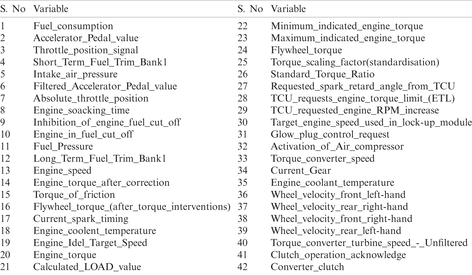
The dataset was taken from [18] and featured 54 parameters and 94,380 values. Validation was conducted using the validation tools MATLAB and Weka.

4.1 Dataset Parameters

The dataset included two basic parameter types: input and output parameters.

4.2 Input Parameters

Tab. 2 presents the external parameters, which pertain to elements external to the driver.

Table 2: Input parameters [18]

4.3 Output Parameters

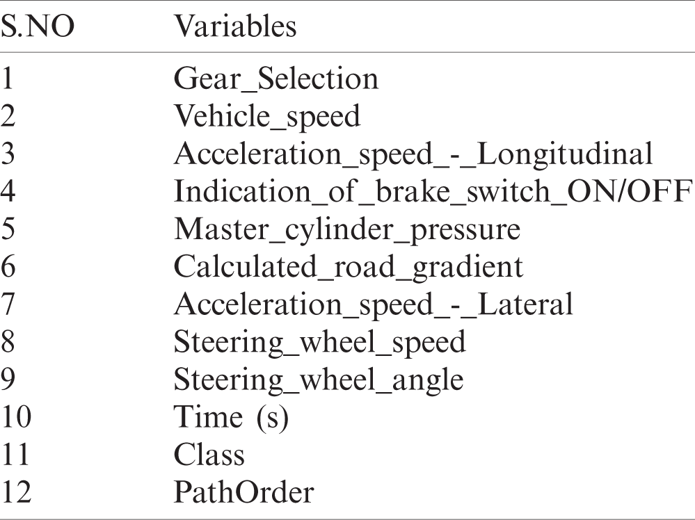
The output parameters presented in Tab. 3 pertain to driver elements.

Table 3: Output parameters [18]

4.4 Validation Techniques

Driver behaviour changes continuously and involves dynamic aspects. Accordingly, a dynamic ANN was used to analyse input values, with results presented according to the real-time scenario.

4.5 Validation Using the MATLAB Time-Series Neural Network

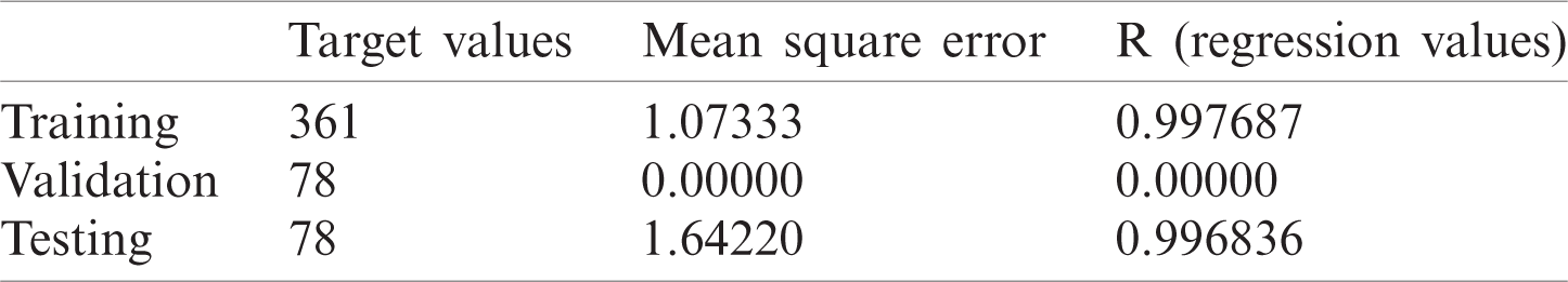
The MATLAB time-series neural network was used to validate the dataset, as presented in Tab. 4. This ANN was chosen because of its dynamic nature; given behaviour is a constantly changing phenomenon, static techniques cannot provide accurate results. Furthermore, the scaled conjugate gradient was chosen for accuracy; this stops automatically when an ANN stops improving following increases in validation values.

Table 4: Validation using MATLAB time-series neural network

4.5.1 Artificial Neural Network Training

The ANN was trained using scaled conjugate gradient. Data division was random, with results presented for 636 epoch iterations. Results included performance, training state, error histogram, regression, time-series response and error autocorrelation.

4.5.2 Training State

The training state graph shows results for epoch 636 and the validation checks at epoch 636. Gradient is on the y-axis, and epoch is on the x-axis. The first graph indicates that values begin at the peak and gradually decrease or minimise.

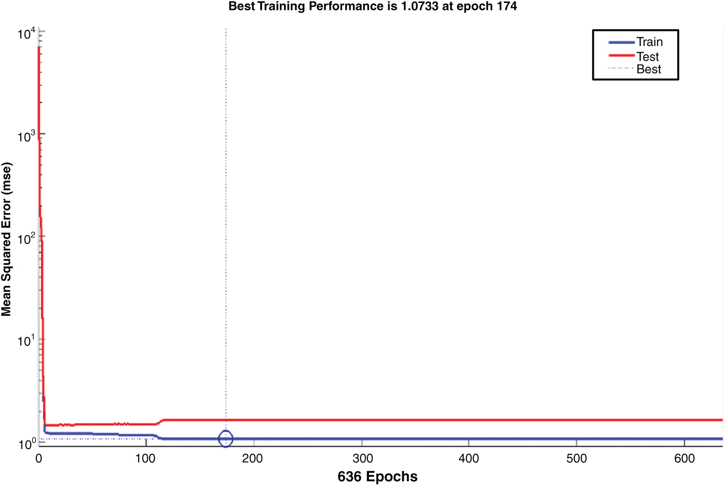
Figure 2: Validation performance: Mean square error decreases as the number of iterations increases

4.5.3 Best Validation Performance

The best validation performance was calculated, as presented in Fig. 2, with the x-axis at epoch 174 and mean square error shown on the y-axis. The best validation performance was calculated as the point at which the best line and the validation line intersected. Overall mean square error tended to decrease as the number of iterations increased.

4.5.4 Error Histogram

The error histogram was computed with 20 bins. At the beginning of the iterations, the minimisation of error tended to increase gradually because training data values increased, and error was totally removed, as shown by the plain orange line. Following the zero error, the training process gradually minimised and totally stopped with only the training state remaining.

4.5.5 Regression Plots

Different regression outputs are shown in Fig. 3, with graph 1 showing the training of data at regression value 0.99769, with the bunching of data indicating the fit line, graph 2 showing the test for fittest data regression values—that is, values nearest to target values—at 0.99684, and graph 3 showing the overall combined result for data flow and regression values at 0.99752; these results are highly refined and accurate.

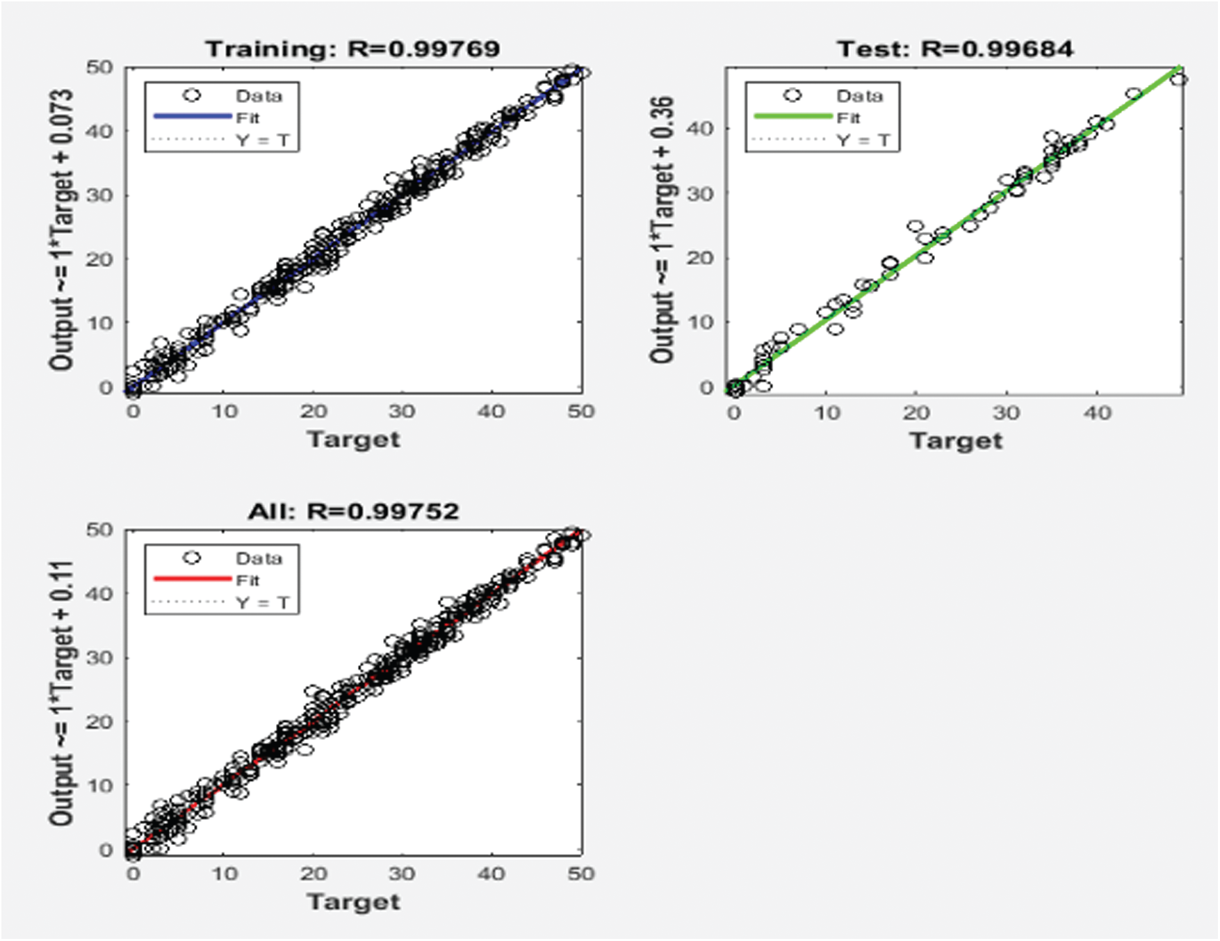
Figure 3: Regression plots

4.5.6 Time-Series Response

Fig. 4 shows the time-series values sequentially by showing the time-series gap between target outputs and training outputs. Variations are indicated clearly for the first half of training; at the beginning of the second half, fluctuations tended to stabilise again.

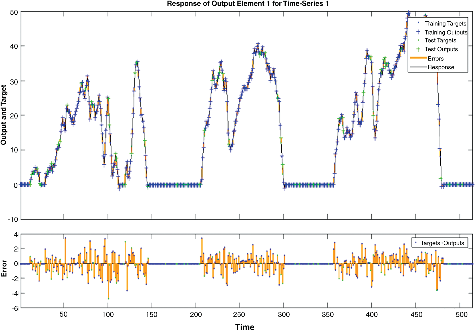
Figure 4: Time-series response showing the time-series gap between target outputs and training outputs

4.6 Validation Using Weka Multilayer Perceptron

Weka is a tool for validating or training neural networks using different training algorithms. This research also used Weka’s multilayer perceptron to train its data.

4.6.1 Pre-Processing

The first step for training in Weka first step is pre-processing the dataset. This involves selecting all filters and attributes to direct classification and clustering.

4.6.2 Classification

The second step is classifying the dataset. There were 54 attributes that could be trained for 31 sigmoid nodes. Results are given in the following sections.

4.6.3 Classification Results

Tab. 5 presents the results for the classification of training data. The correlation coefficient range was near zero; the closer the result is to zero, the more accurate the ANN training. Mean absolute error and root mean square error are the average means of the error values and range from 0 to 100. Relative absolute error and root relative square error range from 0 to 10.

Table 5: Validation using Weka multilayer perceptron

4.6.4 Cluster

The third step is to cluster the given attributes. This can be conducted using a simple expectation maximisation class, which assigns probability distribution for each instance, indicating the probability of its belonging a different cluster and involves the following steps:

1.    The number of clusters is set to one.

2.    The training set is split randomly into ten folds.

3.    Expectation maximisation is performed ten times using the ten folds in the usual CV manner.

4.    The loglikelihood is averaged across the ten results.

5.    If loglikelihood has increased, the number of clusters is increased by one, and the program continues at step 2.

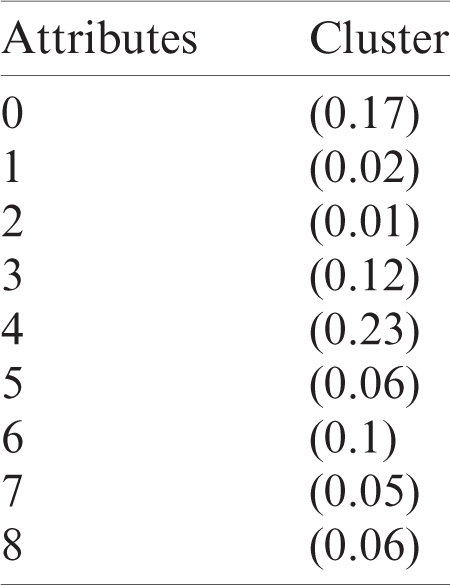
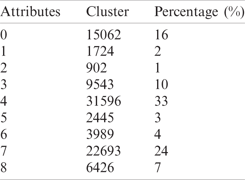
During simulation, the number of clusters selected by cross-validation was nine, the number of iterations performed was three and the loglikelihood value was −47.07798. Tabs. 6 and 7 present the cluster and cluster instance results.

Table 6: Cluster results

Table 7: Cluster instances

4.7 Validation Using Weka Random Subspace

The Weka random subspace approach constructs a decision-tree-based classifier that maintains the highest accuracy for training data and improves generalisation accuracy as it grows in complexity. The classifier comprises multiple trees constructed systematically by pseudo-randomly selecting subsets of components of the feature vector that is tree constructed in randomly chosen subspace.

4.7.1 Classification Results

Results are shown for ten folds and cross-validation techniques. The total classes processed are organised from A to J, with each class showing the individual output values of training iterations in a hierarchical form that indicates tree format.

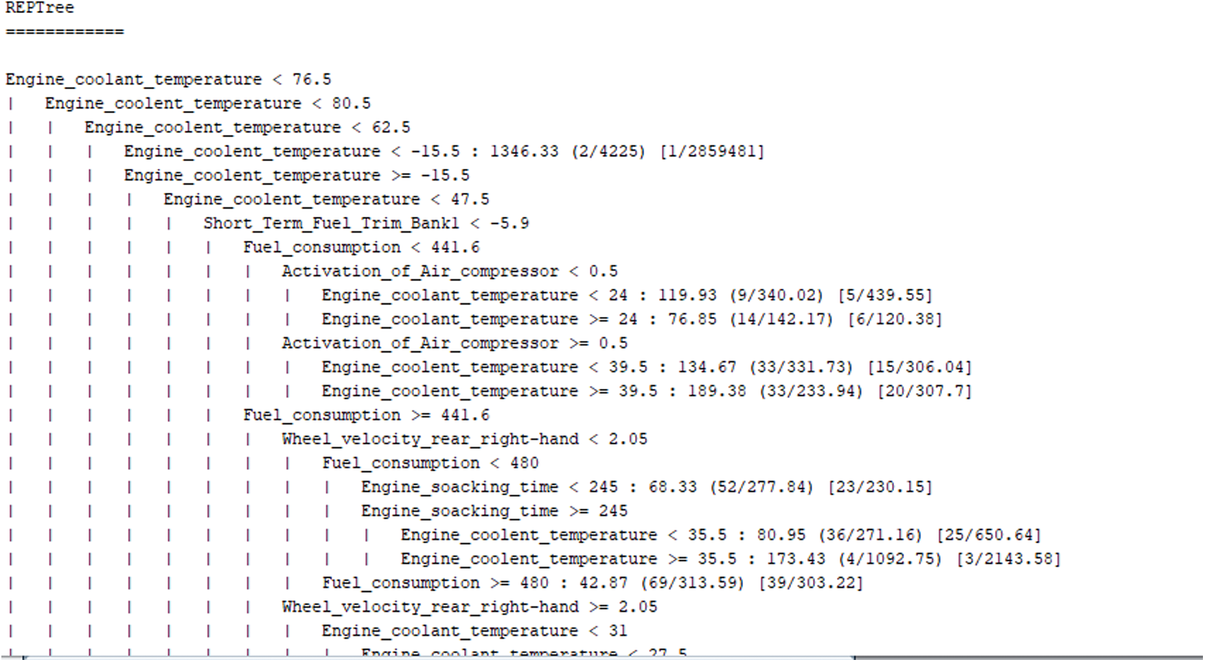
Figure 5: Individual parameter evaluations

The sequence of results for different parameters is shown in Fig. 5; each parameter is evaluated individually for more refined results.

Tab. 8 shows the classification of training data, with the correlation coefficient range being near zero; the closer the result is to zero, the more accurate the ANN training. Mean absolute error and root mean square error are the average means of the error values and range from 0 to 300. Relative absolute error and root relative square error range from 0 to 150.

Table 8: Validation results for Weka random subspace

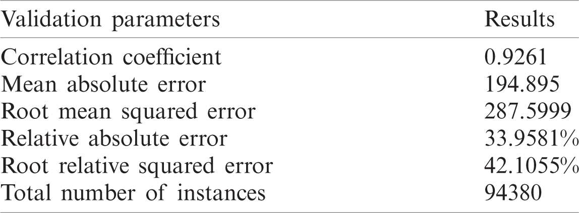
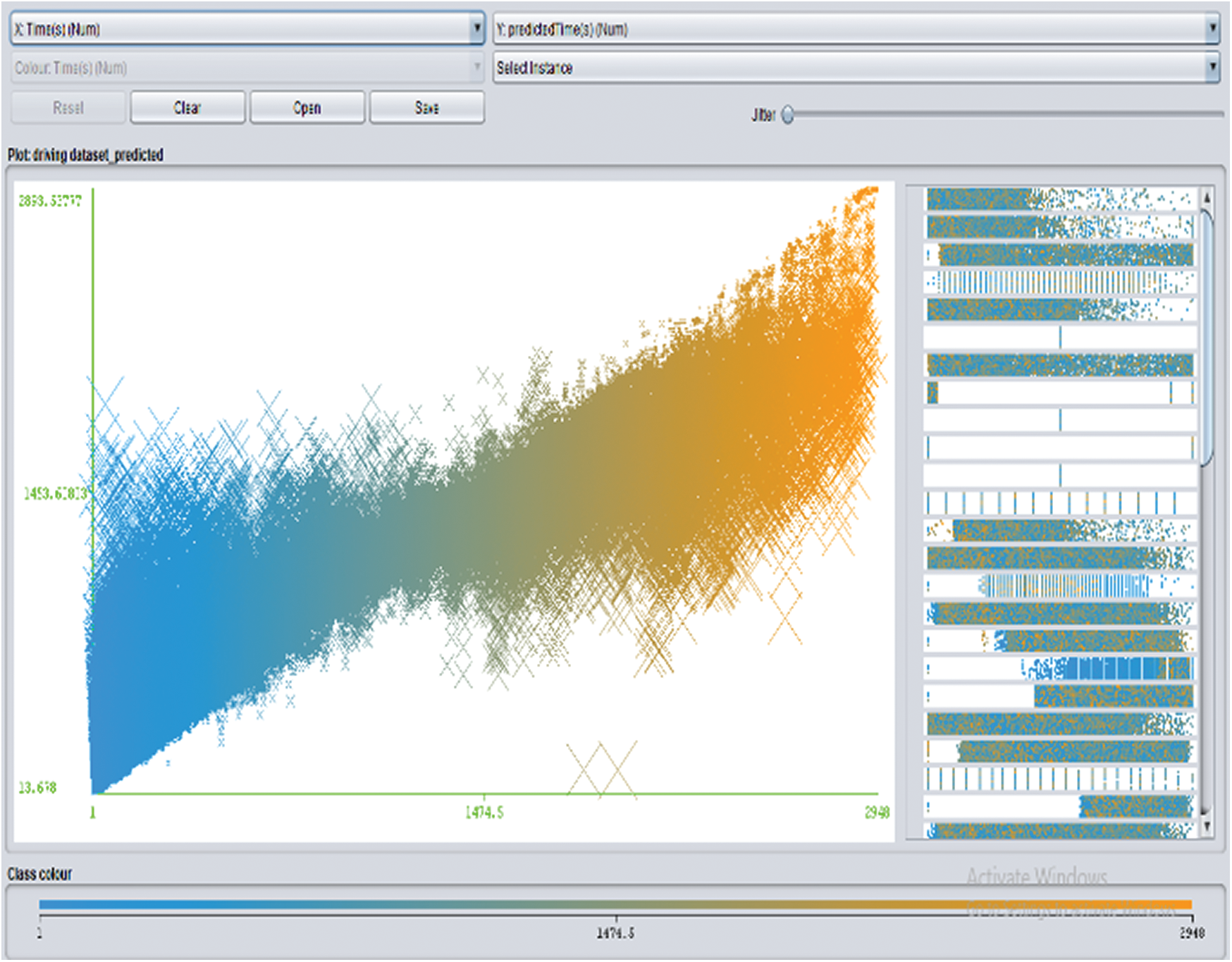
Figure 6: Visualisation comparing time and predicted time: Patterns show the predicted time at different iteration stages

4.7.2 Visualisation

Fig. 6 presents a visualisation of the results in the form of time series. Time is given at the x-axis and predicted time is given at the y-axis. Patterns show the predicted time at different iteration stages.

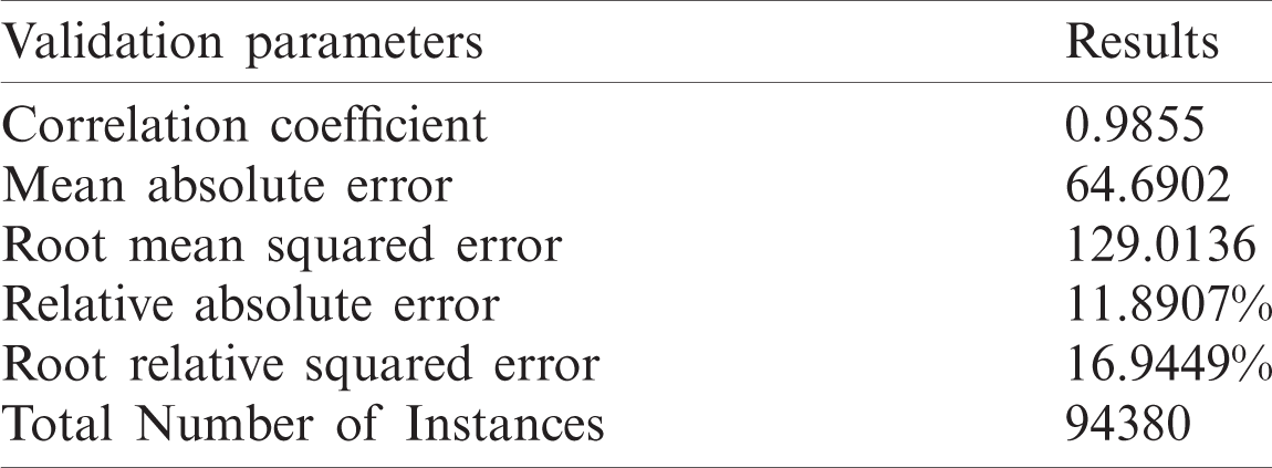
4.8 Validation Using Linear Regression Analysis

Tab. 9 shows the simulation results for linear regression analysis.

Table 9: Validation using linear regression analysis

4.9 Validation Using Decision Tree

Tab. 10 shows the simulation results for the decision-tree approach.

Table 10: Validation using the decision-tree approach

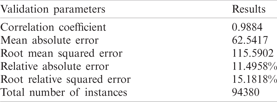
Table 11: Comparison of results

5  Discussion

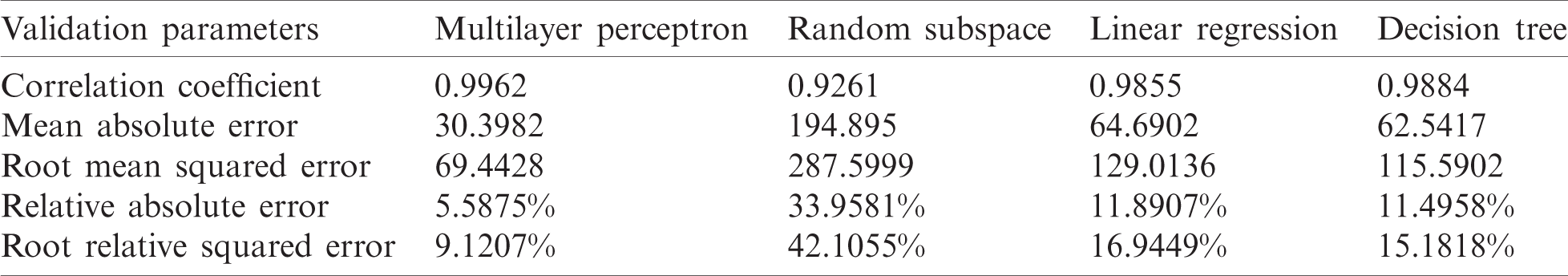
Tab. 11 combines the results of all of the validation techniques used: multilayer perceptron, random subspace, linear regression analysis and decision tree. The differences between the results are indicated by comparing mean absolute errors, root mean square errors, relative absolute errors and root relative squared errors.

Tab. 11 clearly demonstrates that multilayer perceptron produces better results than the other validation techniques.

6  Conclusion

Intelligent agents can represent most human properties due to the similarity in cognitive processes, which enable the completion of deliberate, repetitive tasks ranging from routine to specific tasks. These processes are expressed through intelligent behaviour and actions performed in particular environments. Modelling intelligent driving behaviour is a complex task requiring consideration of many internal and external parameters. These parameters are activated simultaneously to transfer driving patterns from one situation to another, with these patterns constantly evolving to refine driving patterns.

This paper’s ‘driver behaviour model’ can model intelligent driver behaviour in vehicular systems. According to this model, data from a dynamic environment is collected and refined through combination with the driver’s profile and the route details. Refinements of behaviour require intersecting of the model’s decision-making and assistance-system modules, which manage mechanisms internal to driver behaviour and behaviour in emergency situations. The external environment, a driver’s past experience and their current route strongly impact output patterns.

To validate this model, driver datasets comprising multiple values related to different vehicular systems were evaluated, using Weka, by time-series ANNs using MATLAB backpropagation, multilayer perceptron, random subspace, linear regression and decision trees. Results produced means, regressions and correlations using classification and clustering techniques and indicated that the multilayer perceptron approach generates better results than other validation techniques.

Funding Statement: The authors received no specific funding for this study.

Conflicts of Interest: The authors declare that they have no conflicts of interest to report regarding the present study.

This work is licensed under a Creative Commons Attribution 4.0 International License, which permits unrestricted use, distribution, and reproduction in any medium, provided the original work is properly cited.