DOI:10.32604/cmc.2021.015480
| Computers, Materials & Continua DOI:10.32604/cmc.2021.015480 | |
| Article |
A Novel Deep Neural Network for Intracranial Haemorrhage Detection and Classification
1Department of ECE, KPR Institute of Engineering and Technology, Coimbatore, 641407, India
2Department of Electronics and Communication Engineering, University College of Engineering, BIT Campus, Anna University, Tiruchirappalli, 620024, India
3Department of Medical Equipment Technology, College of Applied Medical Sciences, Majmaah University, Al Majmaah, 11952, Saudi Arabia
4Department of Entrepreneurship and Logistics, Plekhanov Russian University of Economics, Moscow, 117997, Russia
5Department of Logistics, State University of Management, Moscow, 109542, Russia
6Department of Computer Applications, Alagappa University, Karaikudi, 630001, India
*Corresponding Author: K. Shankar. Email: drkshankar@ieee.org
Received: 24 November 2020; Accepted: 28 February 2021
Abstract: Data fusion is one of the challenging issues, the healthcare sector is facing in the recent years. Proper diagnosis from digital imagery and treatment are deemed to be the right solution. Intracerebral Haemorrhage (ICH), a condition characterized by injury of blood vessels in brain tissues, is one of the important reasons for stroke. Images generated by X-rays and Computed Tomography (CT) are widely used for estimating the size and location of hemorrhages. Radiologists use manual planimetry, a time-consuming process for segmenting CT scan images. Deep Learning (DL) is the most preferred method to increase the efficiency of diagnosing ICH. In this paper, the researcher presents a unique multi-modal data fusion-based feature extraction technique with Deep Learning (DL) model, abbreviated as FFE-DL for Intracranial Haemorrhage Detection and Classification, also known as FFEDL-ICH. The proposed FFEDL-ICH model has four stages namely, preprocessing, image segmentation, feature extraction, and classification. The input image is first preprocessed using the Gaussian Filtering (GF) technique to remove noise. Secondly, the Density-based Fuzzy C-Means (DFCM) algorithm is used to segment the images. Furthermore, the Fusion-based Feature Extraction model is implemented with handcrafted feature (Local Binary Patterns) and deep features (Residual Network-152) to extract useful features. Finally, Deep Neural Network (DNN) is implemented as a classification technique to differentiate multiple classes of ICH. The researchers, in the current study, used benchmark Intracranial Haemorrhage dataset and simulated the FFEDL-ICH model to assess its diagnostic performance. The findings of the study revealed that the proposed FFEDL-ICH model has the ability to outperform existing models as there is a significant improvement in its performance. For future researches, the researcher recommends the performance improvement of FFEDL-ICH model using learning rate scheduling techniques for DNN.
Keywords: Intracerebral hemorrhage; fusion model; feature extraction; deep features; classification
Traumatic Brain Injury (TBI) is one of the most recorded causes of death worldwide [1]. Patients diagnosed with TBI experience functional disabilities in the long run. When a patient is diagnosed with TBI, the possibilities of having intracranial lesions, for instances Intracranial Hemorrhage (ICH), are high. ICH is one of the severe lesions that causes death. Such a feature is associated with increased mortality rate. Brain injury is highly fatal and leads to paralysis, if left undiagnosed in the earlier stages. Based on the position of brain injury, ICH is classified into five sub-types, which include Intra-Ventricular (IVH), Intra-Parenchymal (IPH), Subarachnoid (SAH), Epidural (EDH), and Subdural (SDH). Generally, the Computerized Tomography (CT) scanning method is used to diagnose critical conditions like TBI. CT scan is accessed easily and the acquisition time of a CT scan is less. Considering these advantages, healthcare professionals prefer CT scan over Magnetic Resonance Imaging (MRI) for early diagnosis of ICH.
During a CT scan, a series of images is generated using X-ray beams. During the scan process, brain cells are captured at various intensities, according to the type of tissue found in X-ray absorbency level (Hounsfield Units (HU)). Such CT scans fall under the application of windowing model. It converts HU values into gray-scale values [0, 255] which depend on window level and width parameters. The diverse features of brain tissues appear in gray-scale image, based on the selection of unique window parameters [2]. In CT scan images, ICH regions are displayed as hyperdense area without any defined architecture. Professional radiologists observe these CT scan images, confirm the presence of ICH, and its type and location. The diagnostic procedure completely depends on the accessibility of a subspecialty-trained neuroradiologist. In spite of these sophistications, there are chances of imprecise and ineffective results, especially in remote areas, where special care is inadequate. Against this backdrop, there is a need persists to overcome this challenge.
Convolutional Neural Network (CNN) is a promising model for automating functions, such as image classification and segmentation [3]. Deep Learning (DL) methods are highly capable of automating ICH prediction and segmentation. The Fully Convolutional Network (FCN) mechanism, otherwise termed as U-Net, is recommended in the literature [4] for segmenting ICH regions in CT scan image. Automated ICH detection and classification are highly helpful for beginners in radiology, when professional doctors are not available during critical situations, especially in developing countries and remote areas. Furthermore, the tool also reduces time and wrong diagnosis, thereby paving a way for quick diagnosis of ICH. It is important to determine the volume of ICH for selecting an appropriate treatment regimen and surgical procedure if any, which aids in brain injury recovery at the earliest.
Several approaches have been proposed in the past to perform automatic ICH segmentation. ICH segmentation models are classified as classical and DL methodologies. In general, conventional approaches preprocess the CT scan images to remove noise, skull and artifacts. In this stage, the image has to be registered, while the brain tissue images should be segmented to extract complex features. These approaches depend on unsupervised clustering for the segmentation of ICH area. Shahangian et al. [5] applied DRLSE to execute the segmentation of EDH, IPH, and SDH regions and proposed a supervised model based on Support Vector Machine (SVM) to classify ICH slices. Brain segmentation was the first procedure in this model that removes both skull and brain ventricles. ICH segmentation was also carried out based on DRLSE. Then, shape and texture features were extracted from ICH regions, and consequently ICH was detected. As a result, the maximum values of Dice coefficient, sensitivity, and specificity were achieved in this study. Additionally, conventional unsupervised models [6] applied Fuzzy C-Means (FCM) clustering technique to perform ICH segmentation.
Muschelli et al. [7] presented an automated approach in which the authors compared various supervised models to propose a model that effectively performs ICH segmentation. Such an approach was accomplished by extracting brain tissue images from CT scans which were first registered through the application of CT brain-extracted template. Several attributes were obtained from every scan. Such features include threshold-related data, such as CT voxel intensity, local moment details, including Mean and Standard Deviation (STD), within-plane remarkable scores, initial segmentation after unsupervised approach, contralateral difference images, distance-to-brain center, and standardized-to-template intensity. The extracted features compared the images of diagnostic CT scan with average CT scan images captured from normal brain tissues. As an inclusion, some of the classifiers applied in this model were Logistic Regression (LR), generalized additive method and Random Forest (RF) method. The above-discussed approach was trained with CT scans and was validated. When compared with other classifiers, RF gained the maximum number of Dice coefficients.
DL models, for ICH segmentation, depend upon CNN or FCN models. In the study conducted earlier [8], two approaches were considered on the basis of CNN for ICH segmentation. Alternatively, secondary model was deployed by Nag et al. in which the developers selected CT slices with ICHs through a trained autoencoder (AE). In this study, ICH segmentation was performed by following an active contour Chan-Vese technology [9]. The study used CT scan dataset and AE was trained using partial data. All these information were applied for performance validation. The study obtained an effective SE, positive predictive value, and a Jaccard index. Furthermore, the study inferred that FCN is capable of detecting ICH in every pixel and can also be applied in ICH segmentation process. Numerous structures of FCNs have been applied earlier in ICH segmentation process, including the Dilated Residual Net (DRN), modified VGG16, and U-Net structures.
Kuo et al. [10] implied a cost-sensitive active learning mechanism which contained an ensemble of Patch-based FCNs (PatchFCN). An uncertain value was determined for every patch and all the patches were consolidated and improved after estimating time constraint. The authors employed CT scan images for training and validation purposes, while retrospective scans and prospective scans were taken for testing. As a result, the study attained the maximum precision in ICH detection using test datasets. However, average precision was accomplished for ICH segmentation. Since the study used cost-sensitive active learning, the performance can be improved by annotating novel CT scans and by increasing the size of training data and scans.
Cho et al. [11] employed CNN-cascade approach for ICH prediction. The study used double FCN methodology for ICH segmentation. CNN-cascade approach depends on GoogLeNet network; whereas dual FCN approach is based on pre-trained VGG16 network. The latter gets extended and fine-tuned under the application of CT slices in brain and stroke images. These models were 5-fold cross-validated using massive CT scans. The researchers performed optimal SE and SP for ICH detection. The study obtained the maximum accuracy from ICH sub-type classification, while from EDH detection, minimum accuracy was achieved. In order to compute ICH segmentation, better precision and recall were determined in the study.
Kuang et al. [12] developed a semi-automated technology for regional ICH segmentation and ischemic infarct segmentation. The model followed U-Net approach for ICH and infarct segmentations. The approach was induced after using ICH and infarct regions for multi-region contour evolution. A collection of hand-engineered features was developed into U-Net based on bilateral density difference among symmetric brain regions in CT scan. The researchers weighed U-Net cross-entropy loss using Euclidean distance between applied pixels and the boundaries of positive masks. Therefore, the proposed semi-automated model, with weight loss, surpassed the classical U-net, where the model gained the maximum Dice similarity coefficient.
The current research study presents a novel Fusion-based Feature Extraction with Deep Learning (DL) model, abbreviated as FFE-DL, for Intracranial Haemorrhage Detection and Classification, known as FFEDL-ICH. The presented FFEDL-ICH model has four stages namely, preprocessing, image segmentation, feature extraction, and classification. In the beginning, the input image is preprocessed using Gaussian Filtering (GF) technique to remove noise. Density-based Fuzzy C-Means (DFCM) algorithm is used for image segmentation. Fusion-based feature extraction model is used with both handcrafted feature (Local Binary Patterns) and deep feature (Residual Network-152) to extract the useful features. Finally, Deep Neural Network (DNN) is applied for classification in which different classes of ICH are identified. The authors simulated the model in benchmark Intracranial Haemorrhage dataset to determine the diagnostic performance of FFEDL-ICH model.
2 The Proposed ICH Diagnosis Model
The ICH diagnosis model, which employs FFEDL-ICH, has four stages namely, preprocessing, segmentation, feature extraction, and classification. Once the input data is preprocessed using GF technique i.e., removal of noise, the quality of the considered image improves. Secondly, the preprocessed images are segmented using DFCM technique to identify the damaged regions. Thirdly, the fused features are extracted and classified by DNN model. During feature extraction, LBP-based handcrafted features and deep features are fused together using ResNet-152 to attain better performance. Fig. 1 shows the overall process involved in the proposed model, whereas the components involved are discussed in the upcoming sections.
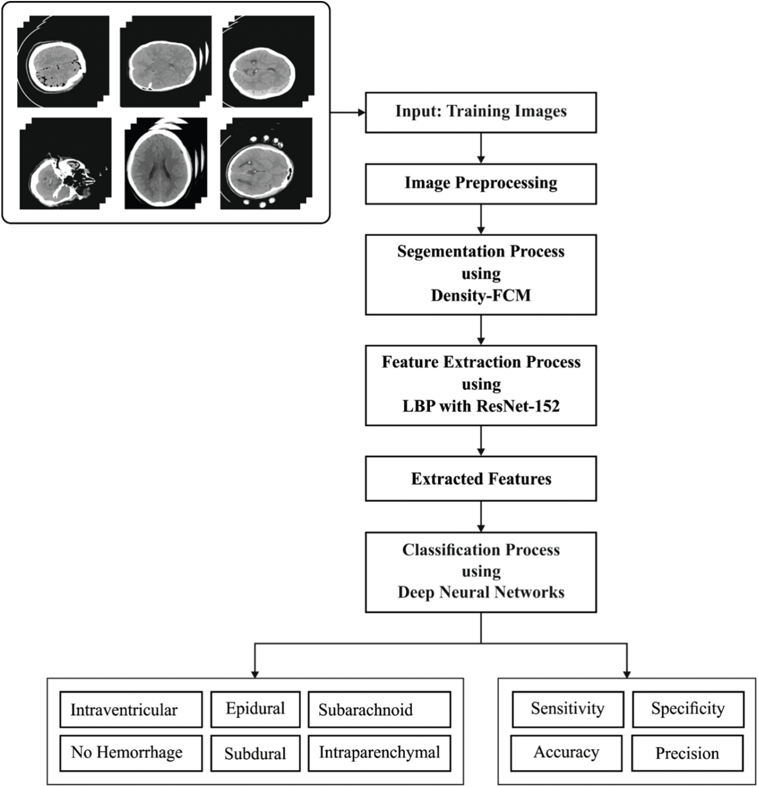
Figure 1: Overall process of FFEDL-ICH
Digital Image Processing technique is applied in a wide range of domains such as astronomy, geography, medicine, and so on. Such models require effective real-time outcomes. 2D Gaussian filter is employed extensively to smoothen the images and remove noise [13]. Such a model necessitates massive processing of resources in an efficient manner. Gaussian is one of the classical operators and Gaussian smoothing procedure is performed by convolution. Gaussian operator, in 1D, is expressed as follows.
An effective smoothing filter is suitable for images in different spatial and frequency domains, wherein the filter satisfies an uncertain relationship, as presented in the equation given below.
Gaussian operator in 2D (circularly symmetric) is depicted as given herewith:
where,
Mean Square Error (MSE) denotes the cumulative square error between the reformed image and the actual image, and is calculated as follows.
where,
Peak Signal-to-Noise Ratio (PSNR) is a peak value of Signal-to-Noise Ratio (SNR) and is defined as a ratio of possible higher power of a pixel value and power of distorted noise. PSNR impacts the supremacy of actual image and is expressed below.
Here,
In this approach, convolution is a multiplication task and provides a logarithmic multiplication. But it remains insufficient to meet the accuracy standards. Therefore, an effective logarithm multiplier is indeed deployed for Gaussian filter, whose accuracy is increased by a logarithm multiplier.
Once the input image is preprocessed, a novel approach called DFCM is employed for image segmentation [14]. When applying FCM method, the count of clusters c as well as primary membership matrix need to be specified, since these values are sensitive in the selection of variables. The two shortcomings develop an effective FCM to compute the optimal clusters, whereas the final outcomes of FCM remain not-so-balanced. Generally, an optimal cluster focuses on partition and relies upon clustering to meet the assumptions made i.e., the initials are nearby true ‘cluster centers’ which are nothing but ‘optimal initials’ with minimum iterations. However, the average description of local data is depicted. Hence, a method for selecting initial cluster centers is presented. During the initial phase, the densities of all samples xi are presented in the form of
where
From Eqs. (6) and (7), it is pointed out that the parameter
As a result, appropriate initial cluster centers are selected from potential cluster centers and the count of clusters c is received simultaneously. The samples can be avoided from a similar cluster, when selecting the initial cluster centers i.e., in case the distance between initial cluster centers is high, it can be selected. It is assumed that the distance between two initial cluster centers has to be higher, compared to the distance threshold as given herewith:
where,
The researcher aims at obtaining an optimal initial membership matrix by eliminating complex functions. In this methodology, initial cluster centers as well as density of sample are provided to develop the basic membership matrix, U. The samples are placed under the cluster in which the center is higher than the considered one. For all the samples in
where,
where,
2.3 Fusion-Based Feature Extraction
In this section, LBP-based handcrafted features and deep features are fused together for effective classification. LBP is often used in image and texture classification processes. LBP is also applied in a number of sectors such as facial analysis, Image Retrieval (IR), palm-print investigation, and so on. LBP has the potential to achieve maximum efficiency and rapid speed within adequate time. It depends on the correlation between intermediate pixels and adjacent neighbors of an image. Therefore, the relationship between intermediate pixels and similar images is related to the boundaries of neighboring and intermediate pixels. When the adjacent pixel gray values are higher than the intermediate pixel, then the LBP bit becomes ‘1’; else it is ‘0’ as showcased in the Eqs. (11) and (12).
where,
where, input image has the size of
Then, deep features from ResNet-152 are extracted. Convolutional Neural Networks (CNN) belong to the family of Deep Learning (DL) methods. CNN can be applied in hierarchical classification operation, specifically, image classification. At first, CNN is developed for image and computer visions with an identical model deployed as visual cortex. CNNs are applied effectively in medical image classification process. In CNNs, an image tensor undergoes convolution using a set of
Every individual matrix Ii is convoluted using a corresponding kernel matrix
In order to reduce the multifaceted processing, CNNs apply pooling layers. At first, the layers are pooled which reduces the size of an output layer from input using a single layer, which is then provided into the system. The current study employed a diverse pooling strategy to reduce the output at the time of protecting important features. In addition, the current study followed Max-pooling approach as well which is an extensively used approach. Higher activation is selected in pooling window. CNN is executed as a discriminative model that applies BP method obtained from sigmoid (Eq. (16)), or Rectified Linear Units (ReLU) (Eq. (17)) activation functions. The consequent layer is composed of a node with sigmoid activation function. It performs binary classification for all classes and a Softmax activation function for multi-class issues as shown in Eq. (18).
In addition, Adam optimizer was employed in this study, which is defined as a Stochastic Gradient Descent (SGD) which applies primary gradient moments (v and m, in Eqs. (19)–(22)). Adam optimizer deals with non-stationarity of a target that is identical to RMSProp, at the time of decomposing sparse gradient issues of RMSProp.
where, mt denotes the initial moment and vt represents a secondary moment and these moments are estimated. ResNet applies the residual block to overcome decomposition and gradient diminishing problems found in CNN. Residual block improves network performance.
Specifically, ResNet networks gain optimal success using ImageNet classification method. Moreover, residual block in ResNet surpasses the additional input and simulation outcome of the remaining blocks as illustrated in Eq. (23):
where, x denotes the input of residual block; W implies the weight of residual block and y shows the final outcome of residual block.
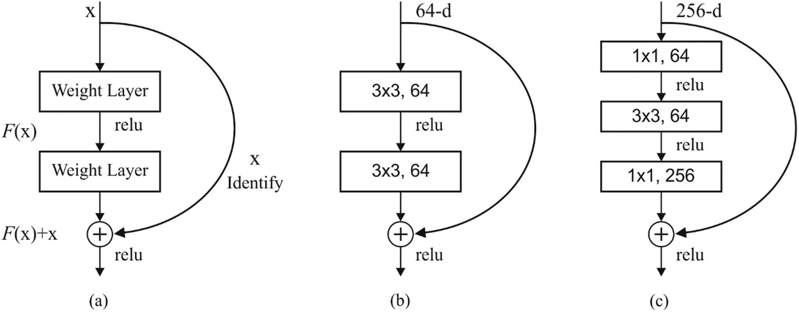
Figure 2: (a) Residual block (b) two layer deep (c) three layer deep
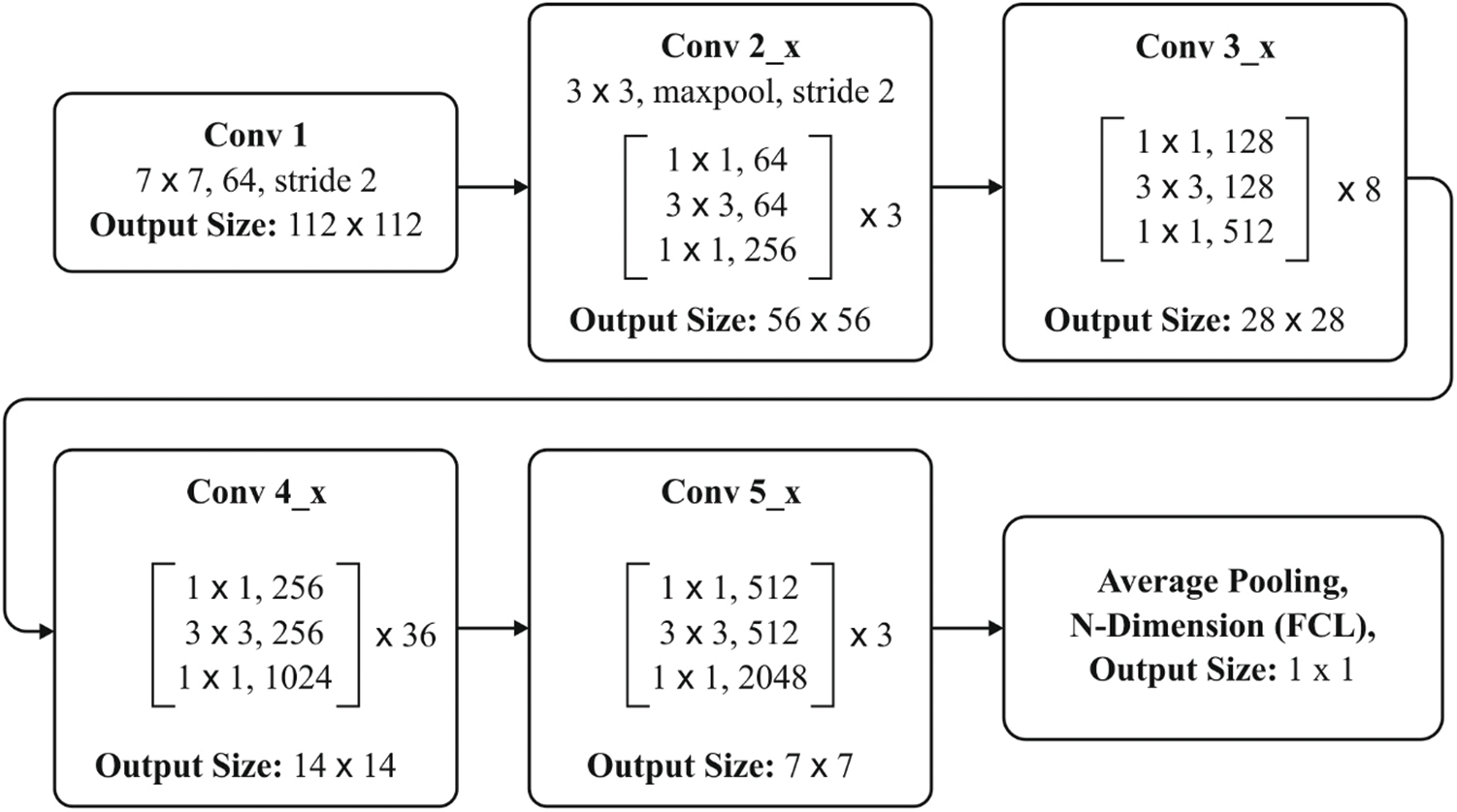
Figure 3: ResNet-152 layers
Fig. 2 shows the block diagram of the newly developed approach. ResNet network is composed of diverse residual blocks, while the size of convolutional kernel is different. ResNet is developed earlier too, in the name of RetNet18, RestNet50, and RestNet152. A common architecture of ResNet152 is shown in Fig. 3. The feature, extracted using ResNet remaining network, is placed in FC layer to classify the images [15]. Hence, DNN method is applied for image classification.
The fusion of features plays a vital role in image classification model that integrates at least two worst feature vectors. Now, features are fused on the basis of entropy. As discussed in earlier sections, LBP and ResNet 152 are fused during fusion process, which is illustrated as follows.
Furthermore, the extracted features are fused in a single vector.
where, f is a fused vector. The fused group of feature vectors is utilized during DNN-based classification process for detecting the existence of ICH.
Feed-Forward Artificial Neural Network (ANN) is a DL model trained with SGD by applying BP. In this model, several layers of hidden units are used between inputs and outcomes [16]. Every hidden unit j, applies the logistic function
In case of multi-class classification like hyperspectral image classification, the output unit j transforms the overall input xj into class probability Pj, with the application of normalized exponential function termed as ‘softmax’
where, h refers to index among all the classes. DNNs are trained in a discriminate manner by BP derivatives of cost function. DNN calculates the discrepancy from target outputs and original outputs are developed for training purpose. While applying softmax output function, natural cost function C is defined as a cross entropy between target probability d and softmax output, P:
Here, the target probabilities consume the values of 1 or 0 and are considered as supervised data offered for training DNN method.
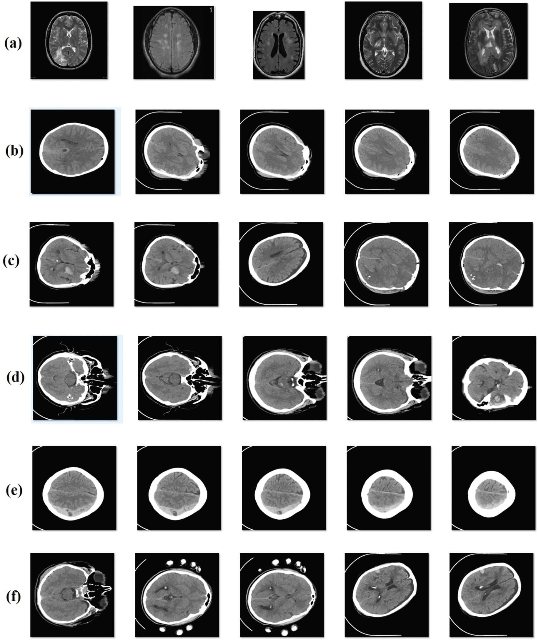
Figure 4: Sample images (a) no hemorrhage (b) epidural (c) intraventricular (d) intraparenchymal (e) subdural (f) subarachnoid
In order to evaluate the performance of the proposed model, an experimental analysis was conducted using a standard ICH dataset [17]. Fig. 4 depicts the sample group of images showing different classes of ICH. CT scan images dataset was collected from 82 patients under the age group of 72 years. Moreover, the dataset is composed of images grouped under six classes, such as Intraventricular with 24 slices, Intraparenchymal with 73 slices, Subdural with 56 slices, Subarachnoid with 18 slices, and No Hemorrhage with 2173 slices. Simulation outcomes were measured in terms of four parameters, such as sensitivity (SE), specificity (SP), accuracy, and precision. To perform the comparative analysis, different methods were used such as U-Net [18], Watershed Algorithm with ANN (WA-ANN) [19], ResNexT [20], Window Estimator Module to a Deep Convolutional Neural Network (WEM-DCNN) [21], CNN and SVM.
Tab. 1 and Fig. 5 represent the performance of FFEDL-ICH model in diagnosing ICH under different number of runs. The simulation outcomes portray that the FFEDL-ICH model achieved the highest ICH diagnosis performance under all the applied runs. For instance, when classifying ICH at run 1, the FFEDL-ICH model reached a higher sensitivity of 95.65%, specificity of 97.98%, precision of 96.09%, and recall of 96.44%. Further, during run 2, ICH was classified by FFEDL-ICH model with superior sensitivity of 95.13%, specificity of 98.12%, precision of 96.31%, and recall of 96.14%.
Table 1: Result of FFEDL-ICH method under different number of runs
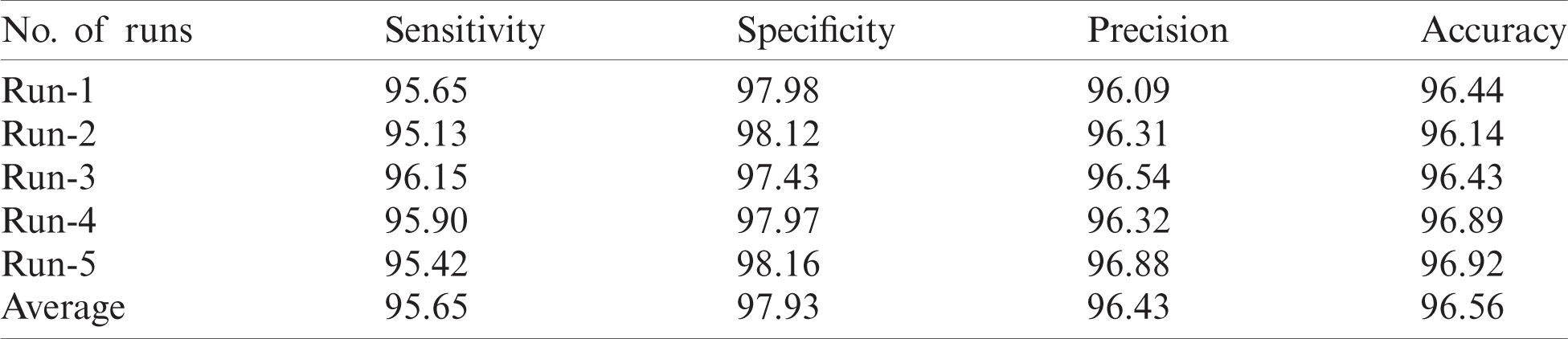
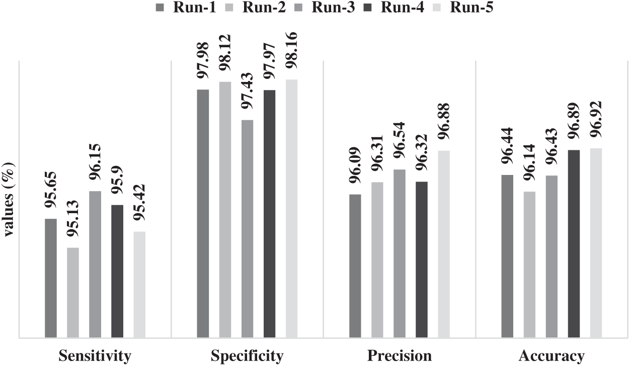
Figure 5: Results of FFEDL-ICH in terms of sensitivity, specificity, precision and accuracy
Likewise, when classifying ICH at run 3, the proposed FFEDL-ICH method achieved a higher sensitivity of 96.15%, specificity of 97.43%, precision of 96.54%, and recall of 96.43%. Even when classifying ICH at run 4, the FFEDL-ICH approach obtained the maximum sensitivity of 95.90%, specificity of 97.97%, precision of 96.32%, and recall of 96.89%. When classifying ICH at run 5, the FFEDL-ICH method accomplished a superior sensitivity of 95.42%, specificity of 98.16%, precision of 96.88%, and recall of 96.92%.
Fig. 6 shows the results attained by FFEDL-ICH model on ICH diagnosis. The experimental outcomes denote that the FFEDL-ICH model produced superior results with high average sensitivity of 95.65%, specificity of 97.93%, precision of 96.43%, and accuracy of 96.56%.
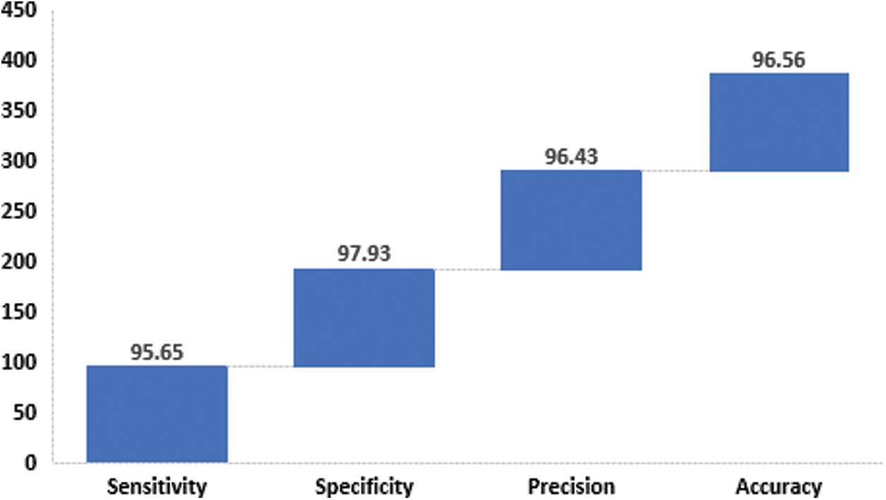
Figure 6: Average analysis of FFEDL-ICH model in terms of sensitivity, specificity, precision and accuracy
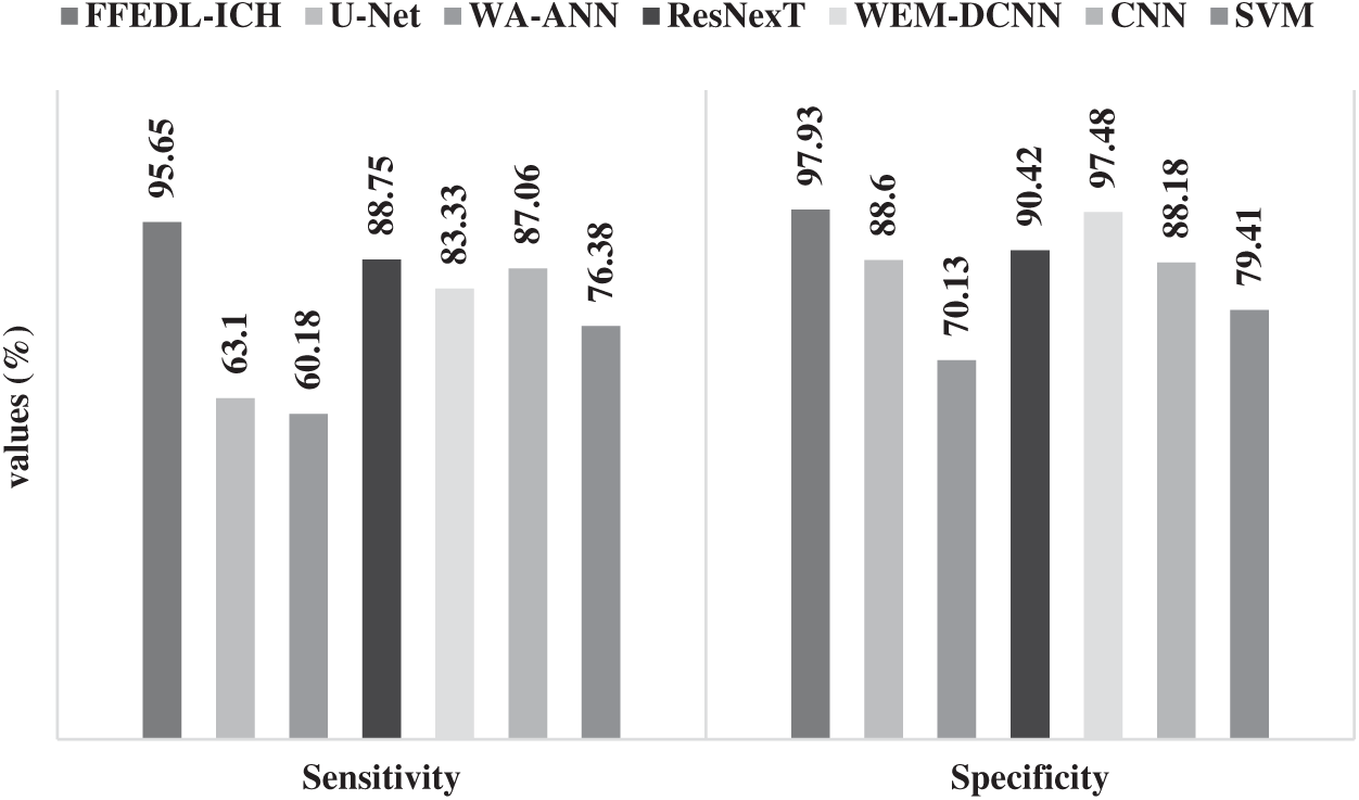
Figure 7: Sensitivity and specificity analyses of FFEDL-ICH model
Fig. 7 shows the results of the analyses yielded by FFEDL-ICH model in terms of sensitivity and specificity. When classifying ICH, in terms of sensitivity, the WA-ANN-based diagnosis model yielded poor results and can be termed as the worst classifier with the least sensitivity of 60.18%. Though U-Net model attempted to outperform the WA-ANN model, it resulted in only a slightly higher sensitivity of 63.1%. Moreover, the SVM model showcased a moderate performance with a sensitivity of 76.38%, whereas the WEM-DCNN model demonstrated somewhat considerable results with a sensitivity of 83.33%. Furthermore, the CNN model exhibited satisfactory results with a sensitivity of 87.06%. In line with these results, the ResNexT model competed well with the proposed model in terms of sensitivity and achieved 88.75%. But the presented FFEDL-ICH model surpassed all the earlier models by achieving the maximum sensitivity of 95.65%.
When classifying ICH using SP, the WA-ANN-relied diagnosis model can be inferred as an ineffective classifier, since it gained the least SP of 70.13%. The SVM method managed to perform well than WA-ANN model, and accomplished a moderate SP of 79.41%. The CNN approach implied a considerable performance with an SP of 88.18%, while the U-Net approach accomplished an acceptable SP outcome of 88.60%. Moreover, the ResNexT framework produced convenient results with 90.42% SP. Along with that, the WEM-DCNN scheme provided a competing result with SP of 97.48%. However, the proposed FFEDL-ICH method outperformed all the compared approaches with the highest SP of 97.93%.
Fig. 8 shows the results of analysis produced by FFEDL-ICH method with respect to precision and accuracy. When classifying ICH by means of precision, the WA-ANN relied on a diagnosis model ended up being an ineffective classifier with the least precision value of 70.08%. The SVM approach managed to perform better than the WA-ANN model and achieved a precision value of 77.53%. Furthermore, the CNN approach produced a considerable performance with a precision of 87.98% and the U-Net model illustrated better results with a precision of 88.19%. The WEM-DCNN technique exhibited reasonable results with a precision of 89.90%. Similarly, the ResNexT approach competed well with a precision of 95.20%. However, the projected FFEDL-ICH framework outperformed other models and achieved an optimal precision of 96.43%.
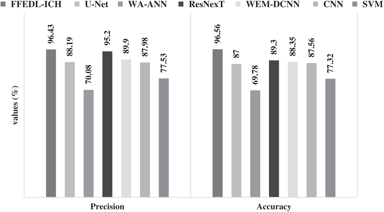
Figure 8: Precision and accuracy analyses of FFEDL-ICH model
When classifying ICH, with respect to accuracy, the WA-ANN related diagnosis model achieved the least position with low accuracy of 69.78%. The SVM technique attempted to perform above WA-ANN approach and yielded a moderate accuracy of 77.32%. Furthermore, the U-Net approach implied a slightly better performance with an accuracy of 87%, whereas the CNN technique accomplished reasonable results with an accuracy of 87.56%. Additionally, the WEM-DCNN method yielded satisfactory outcomes with an accuracy of 88.35%. Likewise, the ResNexT scheme produced competitive results with an accuracy of 89.30%. However, the projected FFEDL-ICH technique performed well than the compared methods and achieved the best accuracy of 96.56%.
The research work presented a DL-based FFEDL-ICH model for detecting and classifying ICH. Four stages present in the proposed FFEDL-ICH model include—preprocessing, image segmentation, feature extraction, and classification. The input image was first preprocessed using GF technique during when the noise was removed to increase the quality of image. Next, the preprocessed images were segmented using DFCM technique to identify the damaged regions. The fused features were then extracted and classified by DNN model in the final stage. The study used Intracranial Haemorrhage dataset to test the effectiveness of the proposed FFEDL-ICH model. The study results were validated under different aspects. The authors infer that the proposed FFEDL-ICH model outperformed all the compared models in terms of sensitivity (SE), specificity (SP), accuracy, and precision. For future researches, the researchers of the current study recommend extending the performance of FFEDL-ICH model using learning rate scheduling techniques for DNN.
Funding Statement: The author(s) received no specific funding for this study.
Conflicts of Interest: The authors declare that they have no conflicts of interest to report regarding the present study.
1. C. A. Taylor, J. M. Bell, M. J. Breiding and L. Xu, “Traumatic brain injury-related emergency department visits, hospitalizations, and deaths-United States, 2007 and 2013,” MMWR Surveill Summ, vol. 66, no. 9, pp. 1–16, 2017. [Google Scholar]
2. Z. Xue, S. Antani, L. R. Long, D. D. Fushman and G. R. Thoma, “Window classification of brain CT images in biomedical articles,” in Annual Sym. Proc. AMIA Sym., Chicago, pp. 1023–1029, 2012. [Google Scholar]
3. G. Litjens, T. Kooi, B. E. Bejnordi, A. A. A. Setio, F. Ciompi et al., “A survey on deep learning in medical image analysis,” Medical Image Analysis, vol. 42, pp. 60–88, 2017. [Google Scholar]
4. O. Ronneberger, P. Fischer and T. Brox, “U-Net: Convolutional networks for biomedical image segmentation,” in Medical Image Computing and Computer-Assisted Intervention—MICCAI 2015: Proc.: Lecture Notes in Computer Science (LNCS, volume 9351New York City, NY, USA, pp. 234–241, 2015. [Google Scholar]
5. B. Shahangian and H. Pourghassem, “Automatic brain hemorrhage segmentation and classification algorithm based on weighted grayscale histogram feature in a hierarchical classification structure,” Biocybernetics and Biomedical Engineering, vol. 36, no. 1, pp. 217–232, 2016. [Google Scholar]
6. A. Gautam and B. Raman, “Automatic segmentation of intracerebral hemorrhage from brain CT images,” in Machine Intelligence and Signal Analysis—Advances in Intelligent Systems and Computing, vol. 748. Singapore: Springer, pp. 753–764, 2018. [Google Scholar]
7. J. Muschelli, E. M.Sweeney, N. L.Ullman, P. Vespa, D. F. Hanley et al., “PItcHPERFeCT: Primary intracranial hemorrhage probability estimation using random forests on CT,” NeuroImage: Clinical, vol. 14, pp. 379–390, 2017. [Google Scholar]
8. P. D. Chang, E. Kuoy, J. Grinband, B. D. Weinberg, M. Thompson et al., “Hybrid 3D/2D convolutional neural network for hemorrhage evaluation on head CT,” American Journal of Neuroradiology, vol. 39, no. 9, pp. 1609–1616, 2018. [Google Scholar]
9. M. K. Nag, S. Chatterjee, A. K. Sadhu, J. Chatterjee and N. Ghosh, “Computer-assisted delineation of hematoma from CT volume using autoencoder and chan vese model,” International Journal of Computer Assisted Radiology and Surgery, vol. 14, pp. 259–269, 2019. [Google Scholar]
10. W. Kuo, C. Häne, E. Yuh, P. Mukherjee and J. Malik, “Cost-sensitive active learning for intracranial hemorrhage detection,” in Medical Image Computing and Computer Assisted Intervention—MICCAI 2018: Proc.: Lecture Notes in Computer Science Book Series (LNCS, volume 11072), New York City, NY, USA, pp. 715–723, 2015. [Google Scholar]
11. J. Cho, K. S. Park, M. Karki, E. Lee, S. Ko et al., “Improving sensitivity on identification and delineation of intracranial hemorrhage lesion using cascaded deep learning models,” Journal of Digital Imaging, vol. 32, pp. 450–461, 2019. [Google Scholar]
12. H. Kuang, B. K. Menon and W. Qiu, “Segmenting hemorrhagic and ischemic infarct simultaneously from follow-up non-contrast CT images in patients with acute ischemic stroke,” IEEE Access, vol. 7, pp. 39842–39851, 2019. [Google Scholar]
13. D. Nandan, J. Kanungo and A. Mahajan, “An error-efficient gaussian filter for image processing by using the expanded operand decomposition logarithm multiplication,” Journal of Ambient Intelligence and Humanized Computing, vol. 2018, pp. 1–8, 2018. [Google Scholar]
14. H. X. Pei, Z. R. Zheng, C. Wang, C. N. Li and Y. H. Shao, “D-FCM: Density based fuzzy c-means clustering algorithm with application in medical image segmentation,” Procedia Computer Science, vol. 122, pp. 407–414, 2017. [Google Scholar]
15. S. Wan, Y. Liang and Y. Zhang, “Deep convolutional neural networks for diabetic retinopathy detection by image classification,” Computers & Electrical Engineering, vol. 72, pp. 274–282, 2018. [Google Scholar]
16. M. S. Roodposhti, J. Aryal, A. Lucieer and B. A. Bryan, “Uncertainty assessment of hyperspectral image classification: Deep learning vs. random forest,” Entropy, vol. 21, no. 1, pp. 1–15, 2019. [Google Scholar]
17. M. Hssayeni, “Computed tomography images for intracranial hemorrhage detection and segmentation (version 1.3.1),” PhysioNet, 2020. https://doi.org/10.13026/4nae-zg36. [Google Scholar]
18. M. D. Hssayeni, M. S. Croock, A. D. Salman, H. F. Al-khafaji, Z. A. Yahya et al., “Intracranial hemorrhage segmentation using a deep convolutional model,” Data, vol. 5, no. 1, pp. 1–18, 2020. [Google Scholar]
19. V. Davis and S. Devane, “Diagnosis & classification of brain hemorrhage,” in 2017 Int. Conf. on Advances in Computing, Communication and Control, Mumbai, India, IEEE, pp. 1–6, 2017. [Google Scholar]
20. G. Danilov, K. Kotik, A. Negreeva, T. Tsukanova, M. Shifrin et al., “Classification of intracranial hemorrhage subtypes using deep learning on CT scans,” Studies in Health Technology and Informatics, vol. 272, pp. 370–373, 2020. [Google Scholar]
21. M. Karki, J. Cho, E. Lee, M. H. Hahm, S. Y. Yoon et al., “CT window trainable neural network for improving intracranial hemorrhage detection by combining multiple settings,” Artificial Intelligence in Medicine, vol. 106, pp. 1–24, 2020. [Google Scholar]
 | This work is licensed under a Creative Commons Attribution 4.0 International License, which permits unrestricted use, distribution, and reproduction in any medium, provided the original work is properly cited. |