DOI:10.32604/cmc.2021.016139
| Computers, Materials & Continua DOI:10.32604/cmc.2021.016139 | |
| Article |
Hybrid Swarm Intelligence Based QoS Aware Clustering with Routing Protocol for WSN
1Department of Computer Science and Engineering, GRT Institute of Engineering and Technology, Tiruttani, 631209, India
2Department of Information Technology, Kongu Engineering College, Erode, 638060, India
3Department of Entrepreneurship and Logistics, Plekhanov Russian University of Economics, Moscow, 117997, Russia
4Department of Logistics, State University of Management, Moscow, 109542, Russia
5Department of Computer Applications, Alagappa University, Karaikudi, 630001, India
*Corresponding Author: K. Shankar. Email: drkshankar@ieee.org
Received: 24 December 2020; Accepted: 04 March 2021
Abstract: Wireless Sensor Networks (WSN) started gaining attention due to its wide application in the fields of data collection and information processing. The recent advancements in multimedia sensors demand the Quality of Service (QoS) be maintained up to certain standards. The restrictions and requirements in QoS management completely depend upon the nature of target application. Some of the major QoS parameters in WSN are energy efficiency, network lifetime, delay and throughput. In this scenario, clustering and routing are considered as the most effective techniques to meet the demands of QoS. Since they are treated as NP (Non-deterministic Polynomial-time) hard problem, Swarm Intelligence (SI) techniques can be implemented. The current research work introduces a new QoS aware Clustering and Routing-based technique using Swarm Intelligence (QoSCRSI) algorithm. The proposed QoSCRSI technique performs two-level clustering and proficient routing. Initially, the fuzzy is hybridized with Glowworm Swarm Optimization (GSO)-based clustering (HFGSOC) technique for optimal selection of Cluster Heads (CHs). Here, Quantum Salp Swarm optimization Algorithm (QSSA)-based routing technique (QSSAR) is utilized to select the possible routes in the network. In order to evaluate the performance of the proposed QoSCRSI technique, the authors conducted extensive simulation analysis with varying node counts. The experimental outcomes, obtained from the proposed QoSCRSI technique, apparently proved that the technique is better compared to other state-of-the-art techniques in terms of energy efficiency, network lifetime, overhead, throughput, and delay.
Keywords: Quality of service; clustering; routing; energy efficiency; wireless sensor networks; swarm intelligence
Wireless Sensor Networks (WSNs) are composed of Sensor Nodes (SN) which are applied in a wide range of applications namely, prediction, processing and communicating the physical parameters of target environment [1]. In the event of high number of sensor nodes and corresponding applications, the chances are high for diverse interruptions when applied in wireless mode. Further, major constraints are also faced, for instance, the application of sensor nodes in specific actions like data accessing, data collection, and memory space. Sensor nodes have diverse specifications like size, processing capability, expense, hardware limitation, power efficiency, and alternate design which tend to complicate the implementation. In addition to these, the energy specification of sensor node is quite complicate in large environment, since it demands concern-based optimization variables. So, it becomes inevitable to develop different Swarm Intelligence (SI) techniques to improve the network lifetime with limited power and concentrate on diverse transmission principles [2].
In the past two decades, various SI models were developed for problem estimation which produced feasible outcomes as well. The recently-developed approaches mostly focus on the strategy of population on the basis of heuristic search models, especially in resolving the optimization issues. SI method works on the basis of behavior of flying birds during resource acquisition available in Low Energy Adaptive Clustering Hierarchy (LEACH) protocol. In such protocols, SI models are used to make different clusters and define the concerned CHs during real-time development of WSN. The lifetime of network gets increased when using different and optimal route detection models. Artificial Bee Colony (ABC) method is a novel mechanism that mimics swarm-based optimization model at the time of monitoring WSN clusters. The unavoidable interruptions, observed in SN, tend to create feasible routes for data transmission to sink node or BS (Base Station). Generally, WSN node is operated as a multi-node pattern; and numerous techniques were developed in the past to route the data and attain the target.
As per the study conducted earlier [3], a significant number of routing techniques track ant behavior as search agent to identify the optimal route for data transfer in WSN. In this study, it is considered that different nodes are stuck due to power scarcity and capability and attempts to route the data through optimal paths. Recently, new imaging techniques are developed using routing-based protocols on the movement of swarms to show superior path and deliver the collected data in the decided path. The method which incorporates nodes in it should be power-saving and robust in nature to collect and send the data. Ant Colony Optimization (ACO) is developed based on behavior of an ant when searching for food. This is a valid solution for diverse route predictions in spite of the fact that this method is unfit for monitoring applications that require timely data transmission. In order to upgrade network implementation, clustering frameworks are connected with the system using hierarchical structures that reduce the basic power consumption. Clustering is a dense compilation of nodes in wide-scale system. In a cluster, only one node is generally selected as Cluster Head (CH), whereas alternate nodes are referred to as Cluster Members (CM). If there is no CH, proactive principle is applied in case of intra-cluster routing. For inter-cluster routing, reactive principle is applied. Moreover, clustering suffers from a wide range of challenges such as assured node connectivity, estimation of best cluster size, and optimization of clustering structures according to the state of CM. In case of hierarchical routing, convention is implemented with CHs.
In WSN, energy efficiency, network lifetime, delay and throughput are the major parameters that correspond to Quality of Service (QoS). The current research work introduces a new QoS aware clustering with routing-based technique using Swarm Intelligence (QoSCRSI) algorithm. The presented QoSCRSI technique follows two-level clustering and proficient routing. Initially, the fuzzy is hybridized with Glowworm Swarm Optimization (GSO)-based clustering (HFGSOC) technique for optimal selection of Cluster Heads (CHs). Next, Quantum Salp Swarm optimization Algorithm (QSSA)-based routing technique (QSSAR) is utilized to select a set of optimum paths in the network. The authors conducted extensive simulation under different node counts in order to assess the performance of the presented QoSCRSI technique.
Yahiaoui et al. [4] presented a QoS-aware clustering routing protocol for actuator networks. Though this protocol provides QoS with respect to delay, this may not be suitable for WSNs. However, it can be employed with heterogeneous features. Subhashree et al. [5] presented a modern version of LEACH model in CH selection. It employs QoS measures like throughput and Packet Delivery Ratio (PDR) to evaluate the function of protocol unlike LEACH method. The objectives of LEACH are to mitigate energy conservation, improve network lifetime, and keep ideal QoS factors. Alnawafa et al. [6] applied a multi-processing LEACH variant protocol to reduce power consumption and enhance the system duration and throughput. QoS parameters were used in this study to validate the performance. Kumar et al. [7] considered the advantages of node power heterogeneity in WSN by developing Energy Efficient Heterogonous Clustered (EEHC) protocol for tri-level system. CH was selected using threshold function based on Residual Energy (RE) available in sensors. Due to the presence of heterogeneity, EEHC is highly efficient compared to LEACH in terms of improved network lifespan. Sharma et al. [8] developed Energy and Traffic and Energy-Aware Routing (TEAR) protocol to elucidate a better interval. In this protocol, SN and random energy levels interrupt the traffic generation value to resolve the limitations of this approach.
Additionally, Dutt et al. [9] established few protocols such as CH Restricted EE Protocol (CREEP), Learning Automata-based Multilevel Heterogeneous Routing (LA-MHR), and Efficient and Dynamic Clustering Scheme (EDCS) for heterogeneous clustering system. Among these protocols, the main objective of CREEP is to reduce the number of CHs for an iteration and to promote the system duration using 2-level heterogeneity. Followed by, multi-level heterogeneous node is projected by LA-MHR, in line with automatic learning. During the implementation of LA-MHR, S-model relies upon learning and cognitive radio spectrum methodologies for CH selection under sink node. Finally, system duration and efficiency were calculated in this study by means of hot spot issue. Likewise, EDCS developed an energy prediction method to save power and maximize the lifespan of network. However, real-time network condition is considered to be dynamic and complex. So, it is highly impossible to extend the network duration.
Hong et al. [10] developed a Clustering-tree Topology Control based on Energy Forecast (CTEF) to resolve some of the issues like network burden, power application through link scalability, PDR, and so on. Additionally, conventional CH selection and cluster evolution apply the main hypothesis and log normal distribution principle to predict accurate mean power of the system. Besides, Moussaoui et al. [11] investigated the characteristics of QoS-based routing protocols in WSNs. In addition, He et al. [12] presented a geographic location-based QoS protocol named SPEED. In this method, the adjacent tables are allocated, while single-hop neighbors are restricted for a node. In Priya et al. [13], multi-objective and multi-constraint optimization routing models were developed. The challenges involved in handling data such as link supremacy and RE measures were regarded as performance metrics to determine the supremacy of the routing protocol. The model ensured robust data delivery and link reliability.
Chen [14] established Self-Stabilizing Hop-constrained Energy efficient (SHE), a complex real-time protocol. After the completion of cluster development, some data packets from CH were included with sink node through diverse paths in this study. Aging Tag (AT) is a technique applied to fulfil the demands of QoS. Eventually, Faheem et al. [15] established Energy-aware QoS routing protocol (EQRP) clustering. Based on the stable structure of protocol, the network was modified using Bird Mating Optimization (BMO) algorithm. Hence, the presented routing protocol established its competency in enhancing throughput, network reliability, limited excess data retransmissions, maximum PDR and minimum ETE delay. Li et al. [16] developed a bi-hop neighborhood data-relied routing protocol. In this research, energy balancing and 2-hop velocity were combined together as a single concept. Consequently, the adaptability was assured when QoS measures are applied in real-time domain.
Fig. 1 shows the overall system architecture of the presented QoSCRSI technique. In general, WSN nodes are arbitrarily placed in the target region and then initialization process is executed to collect the details of neighboring nodes. Next, HFGSOC technique is applied to select two levels of CHs. Then, QSSAR technique is followed to select the optimal routes to destination node. Once the possible routes are selected, the CMs observe the target region, forward the data to CH which then transmits it to BS via inter clusters. This two-level CH selection process takes place in HFGSOC technique. Here, the first-level CHs are selected by following FL technique. Then, the first level CHs undergo GSO-based CH selection process to become the second level CHs.
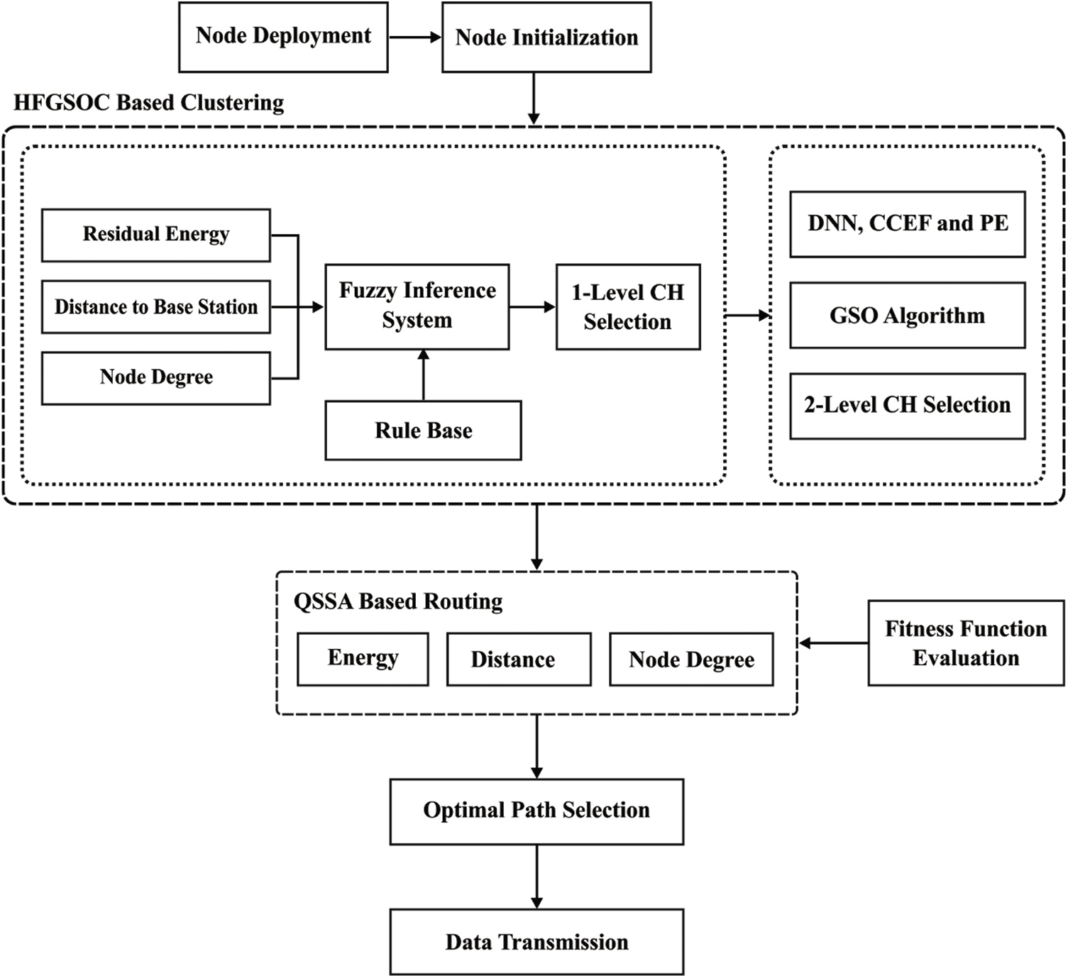
Figure 1: The working process of QoSCRSI model
3.1 Fuzzy Based Level 1 CH Selection
In order to select the first level CHs, FL model makes use of three variables such as RE, Distance To BS (DTBS), and node degree (NDE). Hence, the fuzzy sets are illustrated in Eq. (1).
The pre-defined input fuzzy linguistic parameters are embedded with exclusive membership degree as given herewith.
• RE contains “low,” “medium” and “high;
• DTBS has “close,” “moderate” and “far”;
• NDE is comprised of “low,” “medium” and “high.
Eq. (4) shows the applied Membership Functions (MF) for Fuzzy Inference System (FIS) in triangular MF whereas Eq. (5) shows the Trapezoidal MF (TMF).
The primary objective of FIS is to modify the original input parameters into parallel fuzzy linguistic attributes. In Fuzzy Logic (FL) domain, the most commonly used method is instantiation of linguistic processes like ‘IF premise, THEN conclusion.’ The premise ‘if’ denotes a decision described by fuzzy linguistic variables, whereas ‘conclusion’ defines the fuzzy output variable. Additionally, IF-THEN rule-based knowledge is utilized on the basis of natural language implications. It is deemed that the fuzzy engine evaluates the value of final parameters according to the rules, which leverage the advanced knowledge of evaluation methods. Hence, different types of Mamdani approaches, projected by Takagi-Sugeno-Kang (TSK) fuzzy system, make use of Eq. (6) to evaluate the accurate measure as consequent variable, instead of using fuzzy linguistic parameter.
When TSK model is defined, then the value of y is as given in the Eq. (5).
where m implies the number of fuzzy rules and
A combination of MFs and three attributes such as RE, DTBS and NDE along with previous knowledge of database intend to produce upper function as represented in Eq. (8).
Besides, the least square evaluation for P is attained in which the final attribute is accomplished in TSK fuzzy model. Next, the probability of final value yTSK(X) is determined with the help of Eq. (9).
where
3.2 GSO-Based Level 2 CH Selection
GSO is one of the intelligent swarm optimization models, developed on the basis of luminescent characteristics of fireflies. In GSO method, the glowworms are distributed in solution space and fluorescence intensities are relevant to Fitness Function (FF) value of each glowworm’s location. The optimal position of the glowworm depends upon the intensity of brightness and higher FF value. Every glowworm contains a dynamic line of perception during when the decision domain possesses a range of adjacent nodes. When the density of neighboring node is minimum, then the decision radius might get enhanced. Inversely, decision radius becomes limited, when the glowworms move to same type of robust fluorescence in decision domain.
The model has a total of five states namely, update in fluorescein concentration, neighbor set extension, decision domain radius, moving probability, and glowworm location. Among these, the mechanism behind the upgradation of fluorescein concentration is classified by Eq. (10)
where
where
where rs corresponds to perceived radius of glowworm,
where
In general, the FF of GSO can be applied to overcome the issues in clustering mechanism [18]. Since clustering is a tedious process, massive volume of control data should be fed between the nodes involved in CH selection. This increases the burden of the network. Here, GSO assumes that Deep Neural Network (DNN), Cluster Compactness Estimation Factor (CCEF), and PE are to be selected as Finalized Cluster Heads (FCHs). Once the CH selection is completed, it is then distributed, followed by the removal of imputed data and conjoining of nearby CHs. Here, the energy consumption of CH remains the maximum in comparison with CM. Improper CH selection results in rapid power exhaustion and premature death of CH. This situation can be avoided by proper energy management. Besides, the location of CH should be organized and the size of CH, located nearby sink nodes, should be limited. So, massive CH forwards the data and improves the real-time application. Fig. 2 illustrates the flowchart of GSO method.
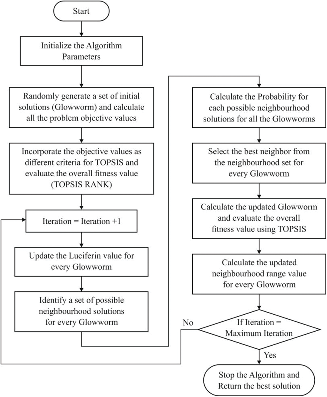
Figure 2: The flowchart of GSO algorithm
Assume N nodes in WSN are deployed as K clusters with
At first, the BS evaluates the high power of nodes, according to the energy available in network. The node with high RE is finalized as the candidate CH. Afterwards, BS applies GSO to perform the clustering by FF as given in Eq. (15).
Local density
where
where f2 illustrates CCEF and low average distance between the node and CH which is determined by Eq. (18).
where
The weight coefficient of estimation factor satisfies
3.3 QSSAR-Based Route Selection Technique
The primary aim of QSSA is to find a novel route from CHS to BS. It is possible to identify a novel path using QSSA as FF metric. This QSSA is composed of RE, distance to BS (DTBS) and NDE. The number of aquatic organisms across the globe outnumber the entire population of human beings itself. However, most of the species follow similar communication models, exhibit identical behaviors, locomotor function and seek food. Salp is a marine species that belongs to Salpidae family. It resembles jellyfishes in structure and cylindrical in shape. There are openings present at the bottom through which the water is pumped through the gelatinous body. The pumped water travels and reaches the inner feeding filters. This marine species exhibit similar behavior alike swarming behavior. For instance, a group of fish is called as shoal of fish while in case of salps, it is named as salp chain. Even though the living atmosphere is highly complicate to access, the biological developers trust that this very characteristic helps the salps to accomplish considerable locomotion and foraging.
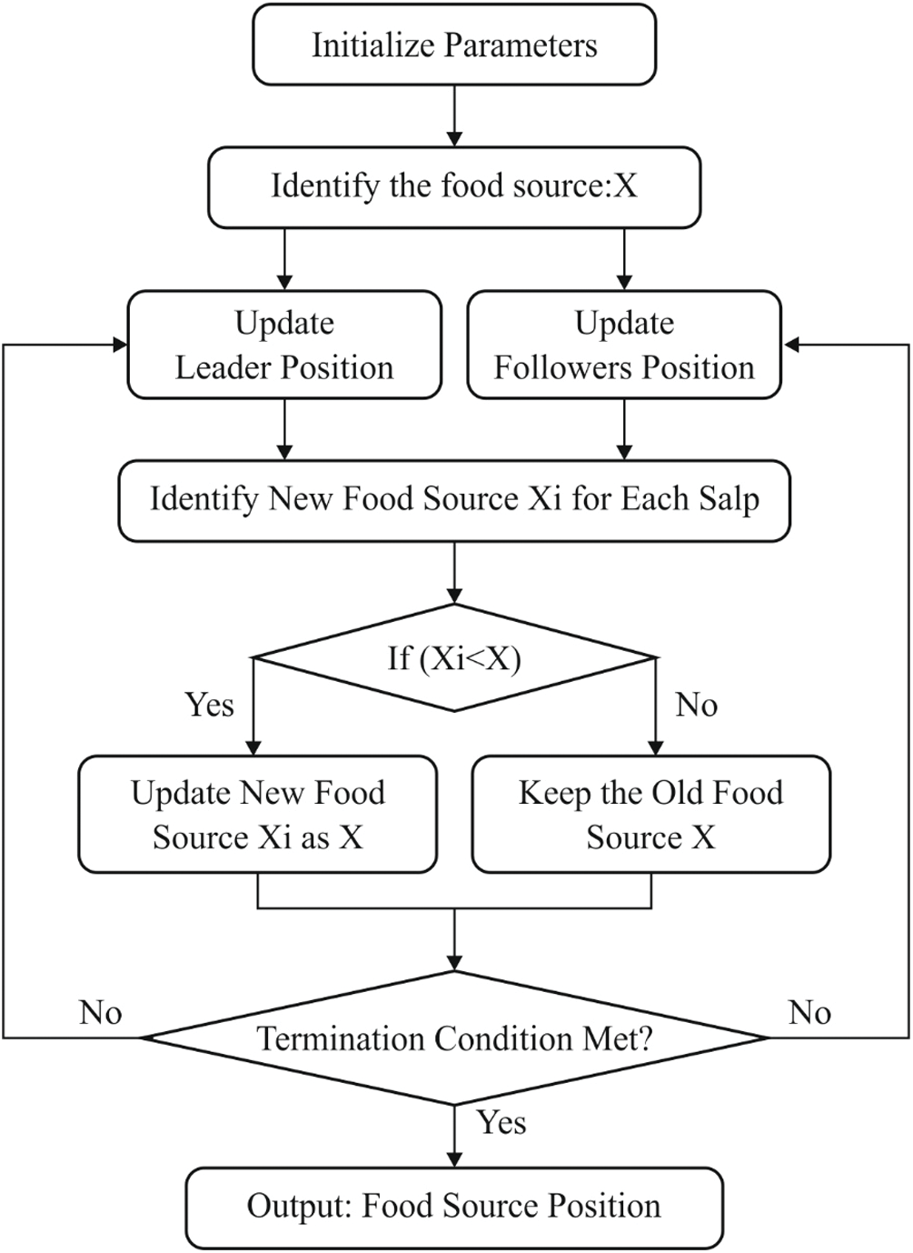
Figure 3: The flowchart of SSA model
Salp Swarm Algorithm (SSA) is a population-relied optimization model. The hierarchy of SSA is better, since it computes salp chain to explore the best food sources. In SSA, the salps are classified into leaders or followers based on the individuals’ (salps) location in the chain [19]. Fig. 3 shows the major phases in SSA. It is initialized by salp population, and swarm X of n salps is depicted in Eq. (20) as 2D matrix. Followed by, the fitness of a salp is determined based on optimal fitness. Hence, the leader position is upgraded by applying Eq. (21).
where
where L represents high iterations and l denotes the recent iteration. It is significant to note that coefficient r1 denotes considerable management between exploration and exploitation in complete search process. Eq. (23) refers to the position update of SSA:
where
where
In order to improve the performance of SSA, QSSA is derived by the incorporation of quantum computing. QSSA is a processing method which applies the models relevant to quantum theory namely, quantum measurement, state superposition and quantum entanglement. qubit is the fundamental unit of quantum processing. The fundamental states |0 > and |1 > make qubit as a linear integration of two basic states as stated herewith.
Quantum gates modify the state of qubits like rotation gate, NOT gate, Hadamard gate, etc. Rotation gate is a mutation operator that develops quanta approach, results in optimal solutions and finally identifies the global best solution [20].
Rotation gate is described herewith.
Here, each FF implies the fittest solution for the applied problem. In routing, every FF denotes the data forwarding route from CH to sink node. The significance of FF is similar to CH available in the network, whereas the excess position is added for sink. The supremacy of FF is same as m + 1, where m denotes the number of CHs involved in the system. Consider,
The identification of optimal route from CH to sink remains the primary task to be achieved. It is attained with the help of FF in different sub objectives like RE, Euclidean distance as well as NDE.
For data delivery, consecutive hop receives the data and transmits it to BS. Therefore, maximum RE of next-hop is prioritized. Also, initial sub objective by means of RE f1 is enhanced by,
It is the distance between CH next hop & sink. When the distance is minimum, the power consumption rate is also less. The second objective is to minimize the distance between CHs and sink. As a result, network lifetime gets maximized and second sub objective refers to the distance of f2 which is measured as follows.
ND denotes the number of CHs with next-hop. If next-hop is comprised of limited CH members, then it consumes low energy in gaining data from adjacent members. It further stays alive for a long period. Therefore, next-hop with limited node degree is chosen prominently. Finally, NDE is defined with respect to node degree i.e., f3 and is expressed as follows
Then, weighted sum model is applied to all sub objectives and are converted as single objective as shown in Eq. (32). Here
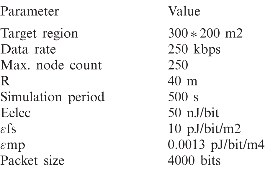
The working function of QoSCRSI method was verified by the researcher under different factors. The newly developed method was simulated under NS2.35 environment. Networks with 50–250 nodes were developed in a random fashion at sensing region. Tab. 1 shows the parameters involved in simulation.
Tab. 2 shows the comparative analysis of QoSCRSI model and existing models under different parameters such as network lifetime, TEC, and throughput analysis. In WSN, the network duration depends upon the count of active nodes and the connectivity between each node.
Fig. 4 shows the results for network duration analysis of QoSCRSI approach under different number of sensor nodes. The figure concludes that ATEER method attained the least duration compared to other schemes. Afterwards, moderate network lifetime was accomplished by OQoS-CMRP technique. Simultaneously, FUCHAR approach yielded a considerable network lifetime, when compared with traditional approaches; however, these values are ineffective compared to the proposed QoSCRSI scheme. The QoSCRSI approach accomplished the highest network lifetime under different count of nodes. For example, under 100 nodes, QoSCRSI model achieved 23993 s. In case of ATEER, OQoS-CMRP, and FUCHAR models, they reached low network lifetime values such as 20105, 21145, and 23073 s correspondingly. Likewise, under 500 nodes, QoSCRSI model gained the maximum network lifetime of 18457 s, while the sensor nodes in ATEER, OQoS-CMRP, and FUCHAR methodologies yielded the least lifetime values of 12619, 14981, and 17875 s correspondingly. Hence, the above values conclude that the QoSCRSI approach has a greater network lifetime than conventional models.
Table 2: Performance analysis of QoSCRSI model with existing techniques
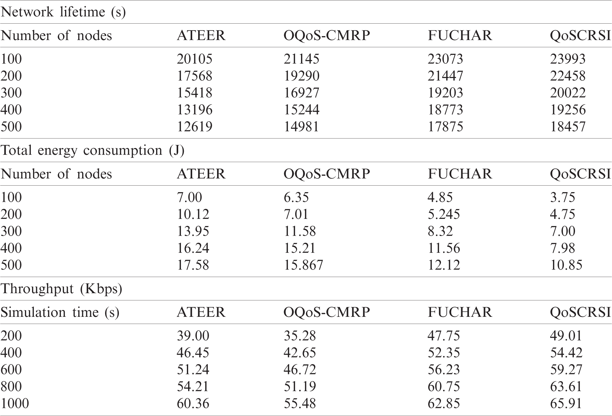
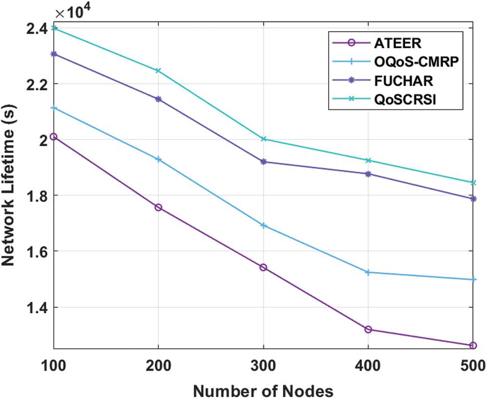
Figure 4: Results of QoSCRSI model in terms of network lifetime
TEC, in sensor nodes, denotes the power expended for sensing, computing, and transmission. The TEC of cluster-based routing protocol should be minimum which implies high power efficiency. Fig. 5 shows TEC investigation of QoSCRSI method and other models under different node counts. From the figure, it is apparent that ATEER model applied high energy than conventional schemes. In line with this, the OQoS-CMRP approach demanded moderate volume of energy, when compared with ATEER, except FUCHAR and QoSCRSI methods. Simultaneously, FUCHAR approach managed to gain low TEC under different node counts. But, the presented QoSCRSI technology accomplished the least TEC compared with other models even under different node counts. For example, under 100 nodes, the QoSCRSI method demanded the minimum TEC of 3.75 J. While ATEER, OQoS-CMRP, and FUCHAR frameworks looked for the maximum TEC values of 7, 6.35, and 4.85 J correspondingly. Similarly, under 500 nodes, the QoSCRSI approach required minimal TEC value of 10.85 J whereas ATEER, OQoS-CMRP, and FUCHAR technologies demanded the maximum TEC values of 17.58, 15.867, and 12.12 J correspondingly. From the result, it can be inferred that QoSCRSI applied the least energy during every performance in the system.
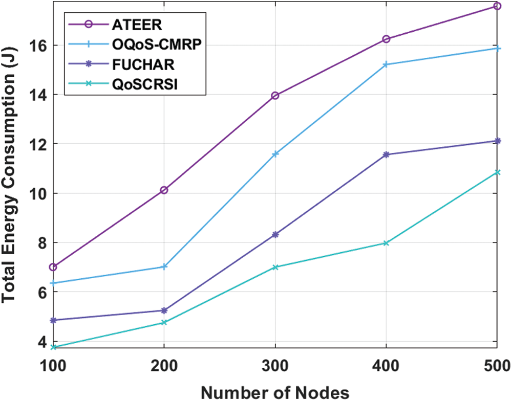
Figure 5: Results of QoSCRSI model in terms of TEC
Fig. 6 shows the results from simulation analysis of QoSCRSI and other compared techniques in terms of throughput. If throughput value is higher, it infers the routing performance is highly productive. The figure depicts that OQoS-CMRP model gained minimum throughput in comparison with previous approaches. The ATEER model exhibited a considerable throughput, when compared with OQoS-CMRP approach. Likewise, the FUCHAR framework offered a moderate throughput than existing schemes, though it was not superior to QoSCRSI model. The proposed QoSCRSI technology achieved high throughput under different counts of nodes. For example, under 200 nodes, the QoSCRSI model accomplished a supreme throughput of 49.01 kbps while ATEER, OQoS-CMRP, and FUCHAR frameworks achieved throughput values of 39 kbps, 35.28 and 47.75 kbps respectively. In line with this, under 1000 nodes, the QoSCRSI technique attained the highest throughput of 65.91 kbps, while the sensor nodes in ATEER, OQoS-CMRP, and FUCHAR models resulted in the least throughput of 60.36, 55.48, and 62.85 kbps, respectively. These values conclude that the proposed QoSCRSI model produced higher throughput over traditional methods.
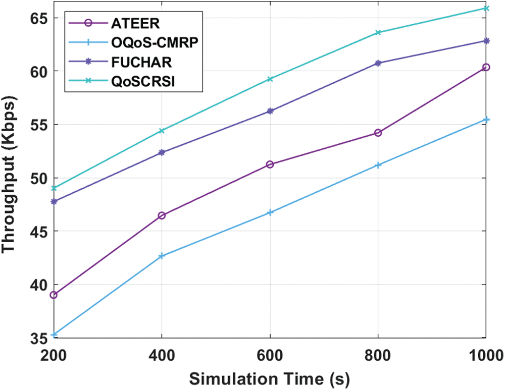
Figure 6: Results of QoSCRSI model in terms of throughput
Fig. 7 shows the results of comparative analysis of QoSCRSI model against existing models under two parameters i.e., Normalized overhead and ETE delay. Normalized overhead is defined as the overall count of control packets that got normalized using whole count of gained data packets. This value infers the results of normalized burden under the existence of different nodes. It further denotes the maximum count of nodes resulted in network overload. Further, the figure conveys that the overhead got maximized further, when the count of nodes was enhanced. It is implied that ATEER and OQoS-CMRP methodologies achieved greater overhead in comparison with conventional methods. At the same time, FUCHAR accomplished a limited overhead than former approaches. However, the newly projected QoSCRSI model obtained a least overhead under diverse scenarios. In case of 100 nodes, the QoSCRSI approach achieved a least overhead of 2.5%, while ATEER, OQoS-CMRP, and FUCHAR models achieved high overhead values of 7.142%, 4.475%, and 4.12% respectively. In line with this, for 500 nodes, QoSCRSI model gained the least overhead of 4.12%, whereas the ATEER, OQoS-CMRP, and FUCHAR approaches achieved the highest overhead of 14.213%, 13.23%, and 6.75% respectively. These values conclude that QoSCRSI does not demand high overhead like other traditional approaches.
ETE delay describes the time consumed by a packet to get transmitted from a node to target in a system. It encloses different types of delays namely, communication delay, queuing delay, processing delay, and so on. ETE delay is applied to exhibit robust features present in routing mechanism. Fig. 7 shows the results of ETE analysis for different methods under distinct simulation time. The figure depicts that the projected QoSCRSI mechanism required only less ETE delay value than the existing technologies. In detail, ATEER and OQoS-CMRP technologies accomplished reasonable and closer ETE delay values, while high ETE delay was achieved by FUCHAR model. For example, under the simulation time of 200 s, the QoSCRSI method attained the least ETE delay of 0.018 s. However, the ATEER, OQoS-CMRP, and FUCHAR methodologies achieved higher ETE delay values of 0.037, 0.035 and 0.028 s correspondingly. In line with this, in case of 1000 nodes, the QoSCRSI approach gained the least ETE delay of 0.021 s, while ATEER, OQoS-CMRP, and FUCHAR frameworks demanded higher ETE delays of 0.044, 0.039 and 0.031 s correspondingly. These values conclude that the proposed QoSCRSI model scheme experienced not much ETE delay compared to other methods. From the results, it is evident that the proposed QoSCRSI approach satisfies QoS demand in terms of power efficiency and ETE delay. Further, it is also established that the QoSCRSI technique is productive compared to other models under different factors such as TEC, ETE delay, overhead, throughput, and network duration. Thus, it can be applied as an efficient cluster-based routing protocol to gain QoS practically.
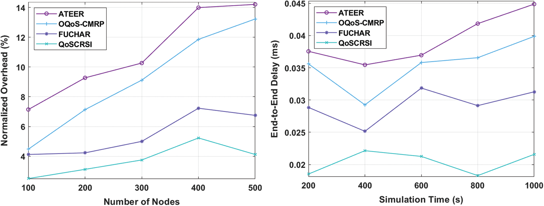
Figure 7: Results of QoSCRSI model in terms of normalized overhead and ETE delay
In current research work, the authors presented a novel QoSCRSI algorithm to satisfy the QoS requirements of WSN. The presented QoSCRSI technique has two-level clustering processes followed by proficient routing process. At first, the nodes in WSN were arbitrarily placed in the target region. Then, the initialization process was executed to collect the details about neighboring nodes. Subsequently, the HFGSOC technique was applied to select the two levels of CHs. Followed by, QSSAR technique was exploited to select the optimal routes for destination node. Once the selection of probable routes was accomplished, the CMs observed the target region, forwarded the data to CH while the latter transmitted the data to BS via inter clusters. The experimental performance of the presented QoSCRSI technique was examined under different node counts. The attained experimental outcomes apparently confirmed that the QoSCRSI technique is superlative compared to other state-of-the-art methods in terms of energy efficiency, network lifetime, overhead, throughput, and delay. In future, data reduction approaches can be exploited to reduce the quantity of redundant data transmission, thereby increasing the energy efficiency.
Funding Statement: The authors received no specific funding for this study.
Conflicts of Interest: The authors declare that they have no conflicts of interest to report regarding the present study.
1. I. F. Akyildiz, W. Su, Y. Sankarasubramaniam and E. Cayirci, “Wireless sensor networks: A survey,” Computer Networks, vol. 38, no. 4, pp. 393–422, 2002. [Google Scholar]
2. D. Caputo, F. Grimaccia, M. Mussetta and R. E. Zich, “An enhanced GSO technique for wireless sensor networks optimization,” in Proc. of the 2008 IEEE Congress on Evolutionary Computation (IEEE World Congress on Computational IntelligenceHong Kong, China, pp. 4074–4079, 2008. [Google Scholar]
3. S. Okdem and D. Karaboga, “Routing in wireless sensor networks using an ant colony optimization (ACO) router chip,” Sensors, vol. 9, no. 2, pp. 909–921, 2009. [Google Scholar]
4. S. Yahiaoui, M. Omar, A. Bouabdallah, E. Natalizio and Y. Challal, “An energy efficient and QoS aware routing protocol for wireless sensor and actuator networks,” AEU International Journal of Electronics and Communications, vol. 83, no. 7, pp. 193–203, 2018. [Google Scholar]
5. V. K. Subhashree, C. Tharini and M. S. Lakshmi, “Modified LEACH: A QoS-aware clustering algorithm for wireless sensor networks,” in Proc. of 2014 Int. Conf. on Communication and Network Technologies, Sivakasi, India, pp. 119–123, 2014. [Google Scholar]
6. E. Alnawafa and I. Marghescu, “New energy efficient multihop routing techniques for wireless sensor networks: Static and dynamic techniques,” Sensors, vol. 18, no. 6, pp. 1863–1883, 2018. [Google Scholar]
7. D. Kumar, T. C. Aseri and R. B. Patel, “EEHC: Energy efficient heterogeneous clustered scheme for wireless sensor networks,” Computer Communications, vol. 32, no. 4, pp. 662–667, 2009. [Google Scholar]
8. D. Sharma and A. P. Bhondekar, “Traffic and energy aware routing for heterogeneous wireless sensor networks,” IEEE Communications Letters, vol. 22, no. 8, pp. 1608–1611, 2018. [Google Scholar]
9. S. Dutt, S. Agrawal and R. Vig, “Cluster-head restricted energy efficient protocol (CREEP) for routing in heterogeneous wireless sensor networks,” Wireless Personal Communications, vol. 100, no. 4, pp. 1477–1497, 2018. [Google Scholar]
10. Z. Hong, R. Wang and X. Li, “A clustering-tree topology control based on the energy forecast for heterogeneous wireless sensor networks,” IEEE/CAA Journal of Automatica Sinica, vol. 3, no. 1, pp. 68–77, 2016. [Google Scholar]
11. A. Moussaoui and A. Boukeream, “A survey of routing protocols based on link-stability in mobile ad hoc networks,” Journal of Network and Computer Applications, vol. 47, no. 1, pp. 1–10, 2015. [Google Scholar]
12. T. He, J. A. Stanko, T. F. Abdelzaher and C. Lu, “A spatiotemporal communication protocol for wireless sensor networks,” IEEE Transactions on Parallel and Distributed Systems, vol. 16, no. 10, pp. 995–1006, 2005. [Google Scholar]
13. S. K. Priya, T. Revathi and K. Muneeswaran, “Multi-constraint multi-objective QoS aware routing heuristics for query driven sensor networks using fuzzy soft sets,” Applied Soft Computing, vol. 52, pp. 532–548, 2017. [Google Scholar]
14. D. R. Chen, “An energy-efficient QoS routing for wireless sensor networks using self-stabilizing algorithm,” Ad Hoc Networks, vol. 37, no. 2, pp. 240–255, 2016. [Google Scholar]
15. M. Faheem and V. C. Gungor, “Energy efficient and QoS aware routing protocol for wireless sensor network-based smart grid applications in the context of industry 4. 0,” Applied Soft Computing, vol. 68, no. 7, pp. 910–922, 2018. [Google Scholar]
16. Y. Li, C. S. Chen, Y. Q. Song, Z. Wang and Y. Sun, “Enhancing real-time delivery in wireless sensor networks with two-hop information,” IEEE Transactions on Industrial Informatics, vol. 5, no. 2, pp. 113–122, 2009. [Google Scholar]
17. S. Arjunan and P. Sujatha, “Lifetime maximization of wireless sensor network using fuzzy based unequal clustering and ACO based routing hybrid protocol,” Applied Intelligence, vol. 48, no. 8, pp. 2229–2246, 2018. [Google Scholar]
18. Y. Xiuwu, L. Qin, L. Yong, H. Mufang, Z. Ke et al., “Uneven clustering routing algorithm based on glowworm swarm optimization,” Ad Hoc Networks, vol. 93, no. 3, pp. 101923, 2019. [Google Scholar]
19. L. Abualigah, M. Shehab, M. Alshinwan and H. Alabool, “Salp swarm algorithm: A comprehensive survey,” Neural Computing and Applications, vol. 32, no. 15, pp. 11195–11215, 2020. [Google Scholar]
20. D. Wang, H. Chen, T. Li, J. Wan and Y. Huang, “A novel quantum grasshopper optimization algorithm for feature selection,” International Journal of Approximate Reasoning, vol. 127, no. 6, pp. 33–53, 2020. [Google Scholar]
 | This work is licensed under a Creative Commons Attribution 4.0 International License, which permits unrestricted use, distribution, and reproduction in any medium, provided the original work is properly cited. |