Computers, Materials & Continua DOI:10.32604/cmc.2021.016362
Article

Phase Error Compensation of Three-Dimensional Reconstruction Combined with Hilbert Transform

Tao Zhang*,1, Jie Shen1 and Shaoen Wu2

1School of Mechanical Engineering, North China University of Water Conservancy and Hydroelectric Power, Zhengzhou, 450045, China
2Department of Computer Science, Ball State University, Muncie, 47306, IN, USA
*Corresponding Author: Tao Zhang. Email: ztncwu@126.com
Received: 31 December 2020; Accepted: 01 March 2021

Abstract: Nonlinear response is an important factor affecting the accuracy of three-dimensional image measurement based on the fringe structured light method. A phase compensation algorithm combined with a Hilbert transform is proposed to reduce the phase error caused by the nonlinear response of a digital projector in the three-dimensional measurement system of fringe structured light. According to the analysis of the influence of Gamma distortion on the phase calculation, the algorithm establishes the relationship model between phase error and harmonic coefficient, introduces phase shift to the signal, and keeps the signal amplitude constant while filtering out the DC component. The phase error is converted to the transform domain, and compared with the numeric value in the space domain. The algorithm is combined with a spiral phase function to optimize the Hilbert transform, so as to eliminate external noise, enhance the image quality, and get an accurate phase value. Experimental results show that the proposed method can effectively improve the accuracy and speed of phase measurement. By performing phase error compensation for free-form surface objects, the phase error is reduced by about 26%, and about 27% of the image reconstruction time is saved, which further demonstrates the feasibility and effectiveness of the method.

Keywords: Three-dimensional reconstruction; structured light; Hilbert transform; phase compensation

1  Preface

Structured light three-dimensional (3D) measurement technology, with non-contact, high-speed, and high-precision measurement, has become a commonly used tool [1–4] in areas such as machine vision, virtual reality, reverse engineering, and industrial measurement. Structured light technology projects a sequence of fringe images on the surface of the measurement object, and the fringe is deformed by the contour of the object. The phase calculation [5–7] of the collected fringe image can realize reconstruction of the three-dimensional contour of the object. However, due to the influence of instrument design, gamma nonlinear distortion [8] between the projector and camera will produce measurement phase errors, and the collected grating fringes will not be an ideal cosine function, but a function with certain distortion. To improve the accuracy of phase calculation requires compensation for the phase error caused by the gamma nonlinear distortion. This has been the topic of much research, mainly of methods of curve calibration, imaging defocusing, and phase error modeling.

Curve calibration makes no changes to the projection fringe pattern, but compensates for the phase error in the phase calculation process. First, the method calibrates a brightness transfer function from projector to camera, and performs a gamma inverse transformation when generating the pattern image to realize advance correction of the input value of the projected image, or gamma correction of a distorted fringe image. Huang et al. [9] established the grayscale mapping relationship between the input fringe image and the fringe image collected by a camera, and deduced the nonlinear phase error caused by nonlinear system response. Guo et al. [10] proposed a technique for gamma correction based on the statistical characteristics of fringe images. Gamma and phase values can be estimated simultaneously through the normalized cumulative histogram of fringe images. Liu et al. [11] modeled the phase error caused by gamma distortion, deduced the relationship between high-order harmonic phase and gamma value, obtained the high-order harmonic phase through a multi-step phase shift, and calibrated the gamma coefficient and performed gamma correction. Li et al. [12] considered the defocusing effect of the projector in the phase error model, for more accurate gamma calibration.

Phase error compensation corrects the projection pattern so that the collected fringe image has an approximately sinusoidal intensity distribution. The phase error is calibrated in advance according to its inherent regularity, and the calculated distortion phase is compensated to obtain the correct phase. Zhang et al. [13] obtained a regular phase error distribution through statistical analysis of the experimental data of a three-step phase shift method, and established a lookup table to compensate for the phase error. Pan et al. [14] pointed out that harmonics higher than the fifth order rarely appear in the digital fringe projection 3D measurement system, so the response signal containing the fifth harmonic is used to derive the phase error model of three-, four-, and five-step phase shift methods. These phase error models are used to design error iteration algorithms, and to calculate the optimal phase.

The defocus imaging method uses the suppression effect of image defocus on high frequency and reduces the high-order harmonic energy of the captured image, thereby reducing the phase error. The method generates a low-pass filter through the defocus of a projector to obtain a fringe image without gamma distortion, thereby avoiding the gamma effect. Zhang et al. [15] used projector defocusing technology to effectively reduce the non-sinusoidal error of fringe images. Zheng et al. [16] binarized grayscale fringes and processed the defocus of the projector to obtain high-quality phase information.

In summary, whether to establish a phase reference, calibrate the gamma value, or defocus projection, auxiliary conditions are needed for phase error compensation. For example, curve calibration and phase error compensation need to quantify the nonlinear response of a system, and defocus imaging method needs to adjust the optical parameters of a system, and both procedures affect a method’s flexibility and robustness.

Current nonlinear phase-error compensation methods all require auxiliary conditions, such as phase reference construction, gamma calibration, and response curve fitting, which affect the flexibility and robustness of the method. This paper presents an adaptive phase error compensation method based on a Hilbert transform. The method introduces a π/2 phase shift in the signal to filter out the direct current (DC) component while the signal amplitude remains unchanged. By comparing the distribution characteristics of the phase error in the Hilbert transform domain and spatial domain, the two domain phases are averaged to compensate for the phase error, without auxiliary conditions.

2  Basic Principle

2.1 Structured Light 3D Reconstruction Error Model

In the structured light 3D reconstruction system, the grating fringes, which are obtained with gamma distortion on the projection reference plane, can be expressed as

Ins(x,y)=A+∑k=1∞[Bk cos(φ+δn)]=α(In)γ(1)

where Ins(x,y) is the fringe gray value distribution, A is the background light intensity, B is the fringe modulation degree, Bk represents the coefficients of the harmonic components in the Fourier series expansion, δn indicates the phase shift of the deformed fringe after modulation, α is a scale factor, ϕ is the ideal phase, and γ is the system gamma value.

According to the principle of least squares, the image data can calculate the package phase information, which can be expressed as

ψ=-arctan(∑i=1N(Ins sinδn)∑i=1N(Ins cosδn))=-arctan(∑n=1N∑k=1∞[Bk cos(ϕ+δn) sinδn]∑n=1N∑k=1∞[Bk cos(ϕ+δn) cosδn])(2)

Due to the nonlinear characteristics of the projection line, the fringe pixel intensity produces nonlinear error. The resulting phase difference is expressed as

Δϕ=ψ-ϕ= arctan(tanψ- tanϕ1+ tanψ⋅ tanϕ)(3)

Substituting Eq. (2) in Eq. (3), the phase difference can be obtained as

Δϕ= arctan(∑n=1N∑k=2∞[(Bk+1-Bk-1) sin(kϕn)]NB1+∑n=1N∑k=2∞[(Bk+1-Bk-1) cos(kϕn)])(4)

The relationship [16] between phase error and GN −1 is given by

Δϕ= arctan{∑m=1∞[(GmN+1-GmN-1) sin(mNϕ)]1+∑m=1∞[(GmN+1+GmN-1) cos(mNϕ)]}(5)

where Gk=BkB1 is a coefficient related to the gamma value. The relationship, which is deduced from Gk and the gamma value [11], is given by

Gk=∏i=2kγ-i+1γ+i(6)

The absolute value of Gk decreases significantly with the harmonic order k. Since GN −1 decreases rapidly with the increase of the number of phase shift steps, and the effect of GN+1 on phase error correction is negligible, considering that the N-order harmonics can already meet the accuracy requirements, Eq. (5) is simplified as

Δϕ= arctan[-GN-1 sin(Nϕ)1+GN-1 cos(Nϕ)](7)

Eq. (7) shows that the phase error is a periodic function related to ideal phase ϕ, phase shift steps N, and gamma value, and its frequency is N times the fringe image, so it is a universal nonlinear phase error model suitable for any number of phase shift steps. Based on this model, different phase-error compensation methods can be proposed according to application requirements.

2.2 Hilbert Transform Compensates Phase Error

The Hilbert transform does not need to rely on external auxiliary conditions to introduce a phase shift in the image signal to compensate for the phase. The Hilbert transform of the phase-shift fringe image is expressed as

InH=H[In]=-Bsin(ϕ+δn)(8)

where InH is the transform image intensity, and H is the Hilbert transform operator. During the Hilbert transformation process, the DC component in the fringe image may not be completely filtered out, and will remain in the transformed image, but it will not affect the phase calculation result because the phase shift method can cancel the DC component. Moreover, when the modulation area of the object to the fringe is less than one fringe period, the Hilbert transform of the fringe image will bring transformation errors. However, in practical applications, dense fringe projection is usually used to obtain high-precision measurements, and the fringe modulation is rarely less than one fringe period.

Due to the nonlinear response, the transformed fringe image also contains high-order harmonics, so the actual transformed image is given by

InHS=H[InS]=-∑k=1∞[Bk sin(kδn)].(9)

According to Eqs. (2)–(7), the actual phase of the transform domain is

ψ= arctan(∑i=1N(Insc cosδn)∑i=1N(Insc sinδn))= arctan(∑n=1N∑k=1∞[Bk sin(ϕ+δn) cosδn]∑n=1N∑k=1∞[Bk sin(ϕ+δn) sinδn])(10)

The phase error in the transform domain is the deviation between the actual phase and true phase. According to the phase derivation formula in the space domain, the phase error is given by

ΔϕH= arctan[GN-1 sin(Nϕ)1-GN-1 cos(Nϕ)](11)

Like the phase error distribution in the space domain, the phase error in the transform domain is a periodic function related to the number of ideal phase shift steps N and the gamma value. By comparing the phase error models in the space domain and transform domain, it can be seen that their amplitudes are equal, but the phase difference is half a period, i.e., the sign is opposite. Therefore, the phase error can be compensated for the help of the Hilbert transform.

Let ψM=(ψ+ψH)/2 be the average phase of the space domain and transform domain. The deviation between the average phase and true phase can be obtained by Eqs. (7) and (11) as

ΔϕM=12arctan[GN-12 sin(2Nϕ)1-GN-12 cos(2Nϕ)].(12)

It can be seen from Eq. (12) that the phase error of the average phase is still a periodic distribution, and its frequency is twice the phase error of the spatial domain. By solving the derivative of the phase errors in Eqs. (7), (11), and (12), the corresponding maximum phase error is obtained. Because |GN-1|<1, the maximum phase error of the average phase is smaller than that of the spatial domain and transform domain. Fig. 1 shows the phase-error distribution curve of the corresponding average phase. It can be seen that this is less than the phase error of the two domains.

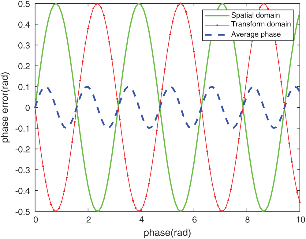
Figure 1: Phase error comparison

2.3 Image Denoising Based on Spiral Phase Function

In an ideal state, the effect of Hilbert transform recovery is good, and there is no need to introduce auxiliary images for processing, but in the Hilbert transform fringe image, there is still a small amount of noise mixed in the eigenmode function components. If one simply applies global mean filtering to the fringes, the overall image will become blurred. Instead of improving the quality, it will reduce the resolution. Moreover, in order to adapt to the needs of images, the Hilbert transform is extended to a two-dimensional space, and its sign function will cause high anisotropy, which cannot meet the requirement of scale invariance. Combining the spiral phase function ϕ(u,v) in the spatial frequency domain, a scale-invariant two-dimensional symbol function is proposed as

SP(u,v)=u+jvu2+v2= exp[jϕ(u,v)](13)

According to Eq. (13), the two-dimensional Hilbert transform operator can be derived as

sH=-jexp(-jβ)F-1{SP(u,v)F[s(x,y)]}(14)

The optimization of the Hilbert transform based on the spiral phase is as follows.

(1) Use the Hilbert spiral to calculate the amplitude distribution of each selected BIMF component and smooth it.

(2) Set a threshold to identify the noise area, and specify that the part whose amplitude distribution is lower than the threshold is noise; the part above the threshold is ignored and not processed.

(3) Smooth the image locally. The identified noise part is subjected to local mean filtering, and the non-noise part is directly used for image reconstruction without processing.

3  Experimental Results and Analysis

To verify the performance of the algorithm, we constructed a structured light 3D measurement system composed of a DLP digital projector BenQ es6299 projector with 1920×1200 resolution, Canon E550D digital camera, and Lenovo T470 notebook computer, as shown in Fig. 2. The period of the projection grating fringe was 50 pixels, the horizontal distance from the projection system to the imaging system d=150 mm, and the distance from the imaging system to the reference surface L=1500 mm. All experiments were carried out on this system.

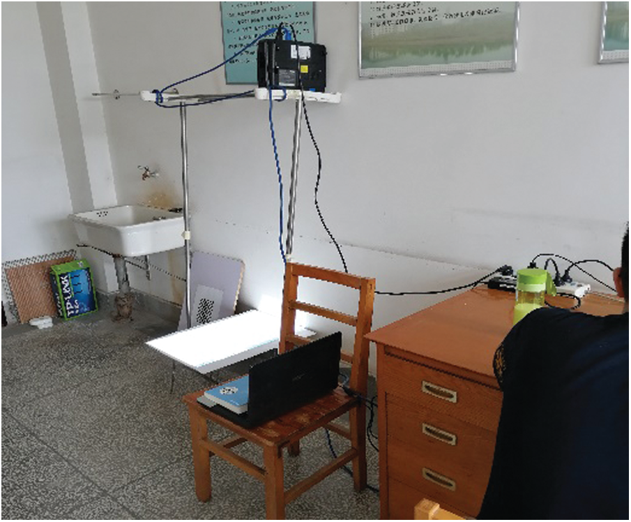
Figure 2: Experimental environment

The system first generated projection grating fringes, where N=60, A=150, B=70. We used simulated fringes to project onto the measurement object, as shown in Fig. 3.

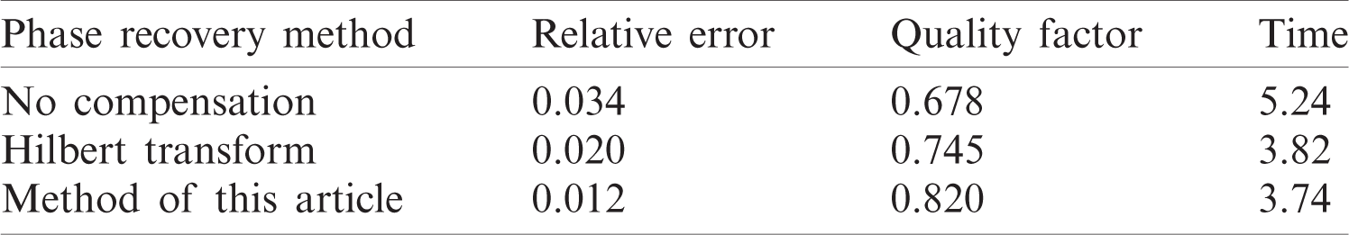
Figs. 4 and 5 show the sinusoidal fringe curve without phase compensation and the generated object profile, respectively. Figs. 6 and 7 are the sinusoidal fringe curve and the generated object contour after phase compensation using the Hilbert transform, respectively. After compensation, the phase error was reduced, but due to the influence of other error sources, such as sensor noise, quantization error, and ambient light interference, the extracted object contour still had a small amount of error. Figs. 8 and 9 are respectively the sinusoidal fringe curve and the generated object profile after phase compensation using the method in this paper. Because the image quality was improved before the Hilbert transform, the phase error of the sine fringe was greatly reduced, the object contour became smooth, and the noise was eliminated.

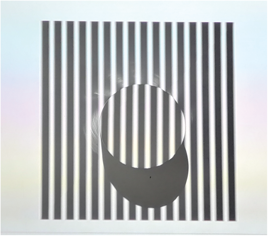
Figure 3: Image with stripe structured light

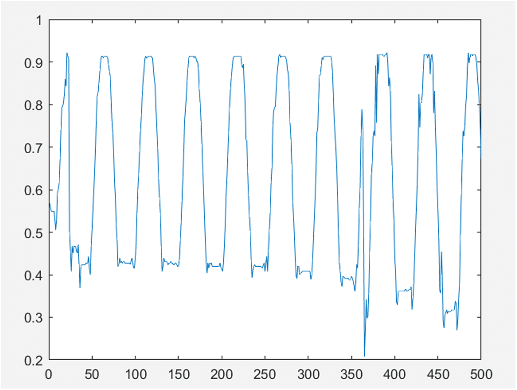
Figure 4: Sinusoidal fringe curve without phase compensation

To more accurately reflect the effect of phase recovery, the relative error RMSE and image quality factor Q are introduced as evaluation criteria. The relative error RMSE is the expected value of the square of the image error,

RMSE=1m*n∑im*n(xi-yi)2(15)

where x and y are the original signal and compensation signal, respectively, and m*n is the image size. The image quality factor does not depend on external observation conditions. It is a standard to evaluate whether the image is distorted and an objective indicator for evaluating the quality of image restoration. It is defined as

Q=4σxyx¯y¯(σx2+σy2)(x¯2+y¯2)(16)

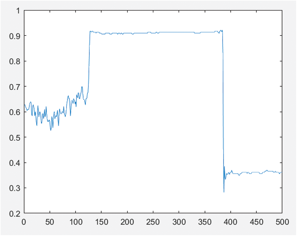
Figure 5: Object profile in cross-sectional direction

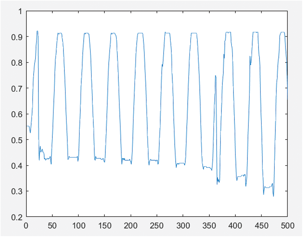
Figure 6: Sinusoidal fringes using Hilbert transform

where x¯ and y¯ are the average values of the original signal and compensated signal, respectively; σx and σy are the variances of the two images; and σx,y is their covariance. The range of Q is [ −1, 1]. When Q is equal to 1, it is the optimal value, i.e., when the variances of the two images are equal, the best value is used. At this time, the image compensation effect is the best. In addition, the time consumed by various methods to restore the phase is also counted. The specific data is shown in Tab. 1.

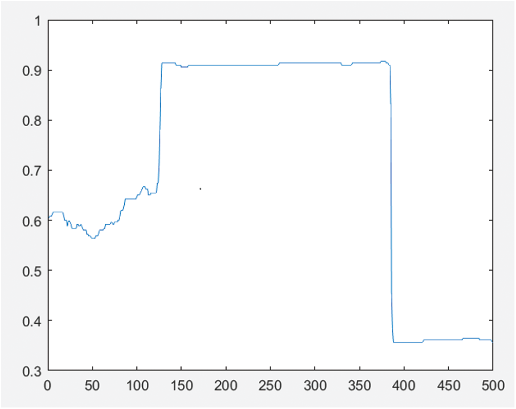
Figure 7: Object profile in cross-sectional direction

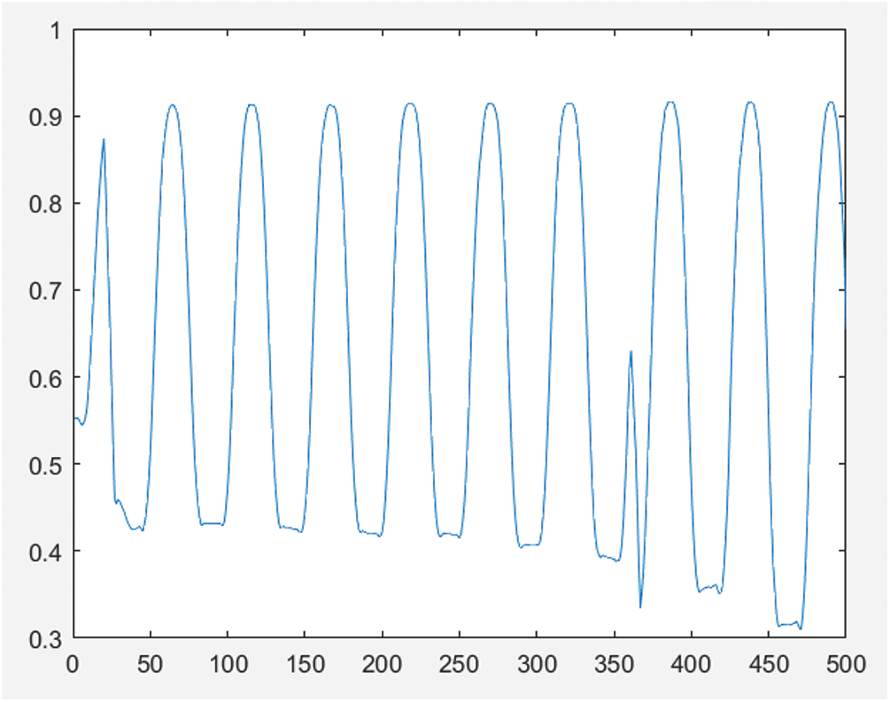
Figure 8: Sinusoidal fringe curve using this method

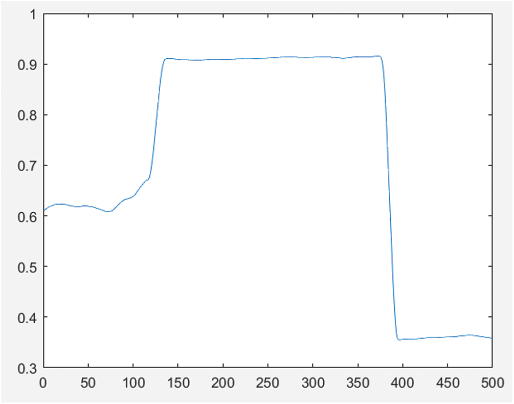
Figure 9: Object profile in cross-sectional direction

Table 1: Comparison of phase recovery of various methods

4  Conclusions

Gamma nonlinearity may result in phase error in a structured light 3D reconstruction system. The phase model and phase error model of gamma distortion are derived from the analysis of the relationship between the gamma distortion and phase error. A nonlinear phase error compensation method based on a Hilbert transform was proposed, making use of the property of the Hilbert transform that induces a phase shift of 2π to a signal, and comparing the nonlinear phase error in the spatial domain and the Hilbert transform domain. By combining the method with the spiral phase algorithm to further improve the image quality, rapid phase compensation was realized to improve the quality of the reconstructed phase.

Acknowledgement: The authors thank Dr. Jinxing Niu for his suggestions. The authors thank the anonymous reviewers and the editor for the instructive suggestions that significantly improved the quality of this paper. We thank LetPub (www.letpub.com) for its linguistic assistance during the preparation of this manuscript.

Funding Statement: This work is funded by the Scientific and Technological Projects of Henan Province under Grant 152102210115.

Conflicts of Interest: The authors declare that they have no conflicts of interest to report regarding the present study.

This work is licensed under a Creative Commons Attribution 4.0 International License, which permits unrestricted use, distribution, and reproduction in any medium, provided the original work is properly cited.