DOI:10.32604/cmc.2021.016893
| Computers, Materials & Continua DOI:10.32604/cmc.2021.016893 | |
| Article |
Enhanced Accuracy for Motor Imagery Detection Using Deep Learning for BCI
1National University of Sciences and Technology (NUST), Islamabad, 44000, Pakistan
2Department of Software, Sejong University, Seoul, Gwangjin-gu, Korea
3College of Computer Engineering and Sciences, Prince Sattam bin Abdulaziz University, Al-Kharj, 11942, Saudi Arabia
*Corresponding Author: Oh-Young Song. Email: oysong@sejong.ac.kr
Received: 14 January 2021; Accepted: 01 March 2021
Abstract: Brain-Computer Interface (BCI) is a system that provides a link between the brain of humans and the hardware directly. The recorded brain data is converted directly to the machine that can be used to control external devices. There are four major components of the BCI system: acquiring signals, preprocessing of acquired signals, features extraction, and classification. In traditional machine learning algorithms, the accuracy is insignificant and not up to the mark for the classification of multi-class motor imagery data. The major reason for this is, features are selected manually, and we are not able to get those features that give higher accuracy results. In this study, motor imagery (MI) signals have been classified using different deep learning algorithms. We have explored two different methods: Artificial Neural Network (ANN) and Long Short-Term Memory (LSTM). We test the classification accuracy on two datasets: BCI competition III-dataset IIIa and BCI competition IV-dataset IIa. The outcome proved that deep learning algorithms provide greater accuracy results than traditional machine learning algorithms. Amongst the deep learning classifiers, LSTM outperforms the ANN and gives higher classification accuracy of 96.2%.
Keywords: Brain-computer interface; motor imagery; artificial neural network; long-short term memory; classification
Brain-Computer Interface (BCI) is a developing field of exploration that seeks to upgrade the effectiveness and level of computer applications centered on the human. A Brain-Computer Interface based on Motor Imagery (MI) offers ways to express your thoughts to an external system without any vocal communication. For the last two to three decades BCI has gained researcher’s attention and extensive work is done in this field [1–3]. There are many applications of BCI like medicine, education, games, entertainment, and human-computer interaction [4–6]. BCI systems based on motor imagery signals have received a lot of heed in the field of assistive technology. There are two major application categories where MI-based systems are majorly used i.e., for motor action replacement or as a recovery system for motor action recovery.
A BCI framework contains the following components: signal acquiring, signal processing extraction of features, and classification [7]. In Fig. 1, the key components of a BCI system are shown. Whereas, the electrical activity of the brain is recorded in the first part by conducting an experiment or performing some voluntary tasks. Brain signals may be obtained either by invasive or non-invasive approaches. The positioning of electrodes is on the surface of the brain for signal acquisition purposes in the invasive process while in a non-invasive procedure signals are acquired without performing any surgical intervention. With an invasive method, the acquired signal is of better quality, but we prefer the non-invasive method due to its ease of use and implementation. Electroencephalogram (EEG) is one of the most commonly used methods of signal acquiring because of its non-invasive nature, cheapness, and ease of usage. A German psychiatrist Hans Berger for the first time recorded the EEG signals in 1924. EEG is a technique in which electrical impulses from the brain are measured by putting a series of electrodes on the human brain’s surface. The brain signals gather through EEG are then pre-processed. The feature extraction is the next important step after the pre-processing of signals. Different types of features can be removed from pre-processed signals by adopting different feature extraction methods. The features that have been extracted are then given to the classifier for its training. Based on feature values, the trained classifier classifies the human intended actions into one of the predefined classes. The selection of desirable features to obtain the necessary classification results is one of the main challenges in the BCI study.
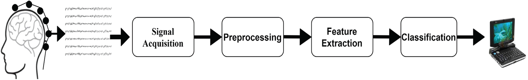
Figure 1: Major components of the BCI system
In traditional machine learning algorithms, the accuracy achieved for the classification of multi-class motor imagery data is insignificant and not up to the mark. The major reason is as features are selected manually, and we are not able to get those features that provide high accuracy results. To overcome this challenge, we proposed an efficient deep learning algorithm. Our contribution included in this article is as follow:
1. A deep learning approach that can be used to manually extract features for the motor imagery signals. The network learns to extract features while training and we just have to feed the signals dataset to the network.
2. By deploying Artificial Neural Network (ANN) and Long Short-Term Memory (LSTM) deep learning algorithms for extracting motor imagery-based features.
Enhanced accuracy for motor imagery detection is a challenging research area in the field of deep learning (DL). For achieving the best accuracy results the desired features are unknown in most of the studies [8]. In the traditional machine learning approach, the features are extracted manually and fed to train the classifier, and we are not able to get those features that provide high accuracy results. Many traditional machine algorithms have already been implemented for the classification of brain signals like support vector machine (SVM) [9], multilayer perceptron (MLP) [10], linear discriminant analysis (LDA) [11].
In another study [8], traditional classifiers like k-NN, SVM, MLP were applied for the classification of signals; the accuracies achieved were not significant enough. In a recent study [12] on EEG data for the classification of motor imagery comparison of traditional and deep learning classifiers was made, the results showed higher accuracies for deep learning classifiers. In our work, we deal with the classification component from brain-computer interface systems with a major focus on deep learning algorithms. In past studies [8], deep learning algorithms have provided better accuracy results in contrast to machine learning algorithms. [13,14] presents different case studies related to machine learning and deep neural networking models. In the deep learning approach, there is no need to manually obtain features from pre-processed signals, the network itself learns to extract the features while training and we just have to feed the dataset to the network. In our study, we analyzed the performance of an artificial neural network (ANN) [15–17] and recurrent neural network (RNN) [18]. Moreover, we implemented long short-term memory (LSTM) [19] in the recurrent neural network. LSTM outperforms ANN and provides higher accuracy results with 96.2%.
During the last decade, a variety of publications have been reported for the classification of multi-class datasets that make use of deep learning [13,14,20,21]. Steady-State Visually Evoked Potential (SSVEP) was used for the classification of EEG based signals in a study [22]. In this work, the subjects were introduced to visual cues at a particular frequency. The accuracy achieved was 97% but the used criteria for reliability rejection was the problem, which resulted in the rejection of a large number of samples resulting in average results. For the classification of data in BCI applications, different approaches have been used like learning vector quantization (LVQ) [23] and CNN [24]. In another study [25], RNN is used for the classification of motor imagery EEG-based data set the accuracy achieved was 79.6% and wavelet filter was used. In a recent work [26], CNN-LSTM based deep learning classifier was used and the maximum test accuracy was targeted at 86.8%. EEG signals were extracted using low cost and invasive headbands in the study.
The next Section 3 summaries the detail of the datasets used in this work, their time paradigm for the collection of raw data from the experiment, and pre-processing steps applied to the raw dataset. After datasets, there is an explanation of both the architectures used in this work. The detailed accuracy results of both the datasets using different architectures and window sizes along with their accuracy and loss graphs are presented in Section 4. Conclusions and discussion are described in Section 5.
In this section, we have discussed all the datasets used in this work, their preprocessing. The datasets involved in the BCI dataset and preprocessing include competition III, dataset IIIa and BCI competition IV, dataset IIa. There is a discussion on the time paradigm and steps involved in the preprocessing of both datasets. Afterward, we have discussed the methodology that has been used in this study. We worked on two algorithms i.e., Artificial Neural Network (ANN) and Long-Short Term Memory (LSTM) for the classification of the datasets. The details are discussed later in this section.
3.1 BCI Dataset and Preprocessing
There are two MI-based four-class datasets used in this work. Both the datasets consist of multiple subjects. The four-class motor imagery corresponds to the MI movement i.e., the right hand, left hand, tongue, and feet. The first dataset used is the IIIa dataset [27] from the third competition of BCI and it comprises 3 subjects. The second dataset IIa [28,29] is from the fourth BCI competition and it consists of 9 subjects. Both the datasets used in this work were available publicly by the Graz University of Technology. Based on a visual cue shown to the participants, all the subjected were asked to carry out four unalike imagery tasks during the experiment. In the next section, there is a detail of both the datasets used, their design.
3.1.1 BCI Competition III, Dataset IIIa
1) Paradigm
The experiment starts with the subject sitting on a relaxing chair. According to a cue, imagery movements i.e.,, left hand, right hand, tongue, and foot were asked to perform. The cues were shown randomly. There were 6 runs and each run contained 40 trials. Each trial comprises of 8 s in total. The first 2 s were blank and quiet, at
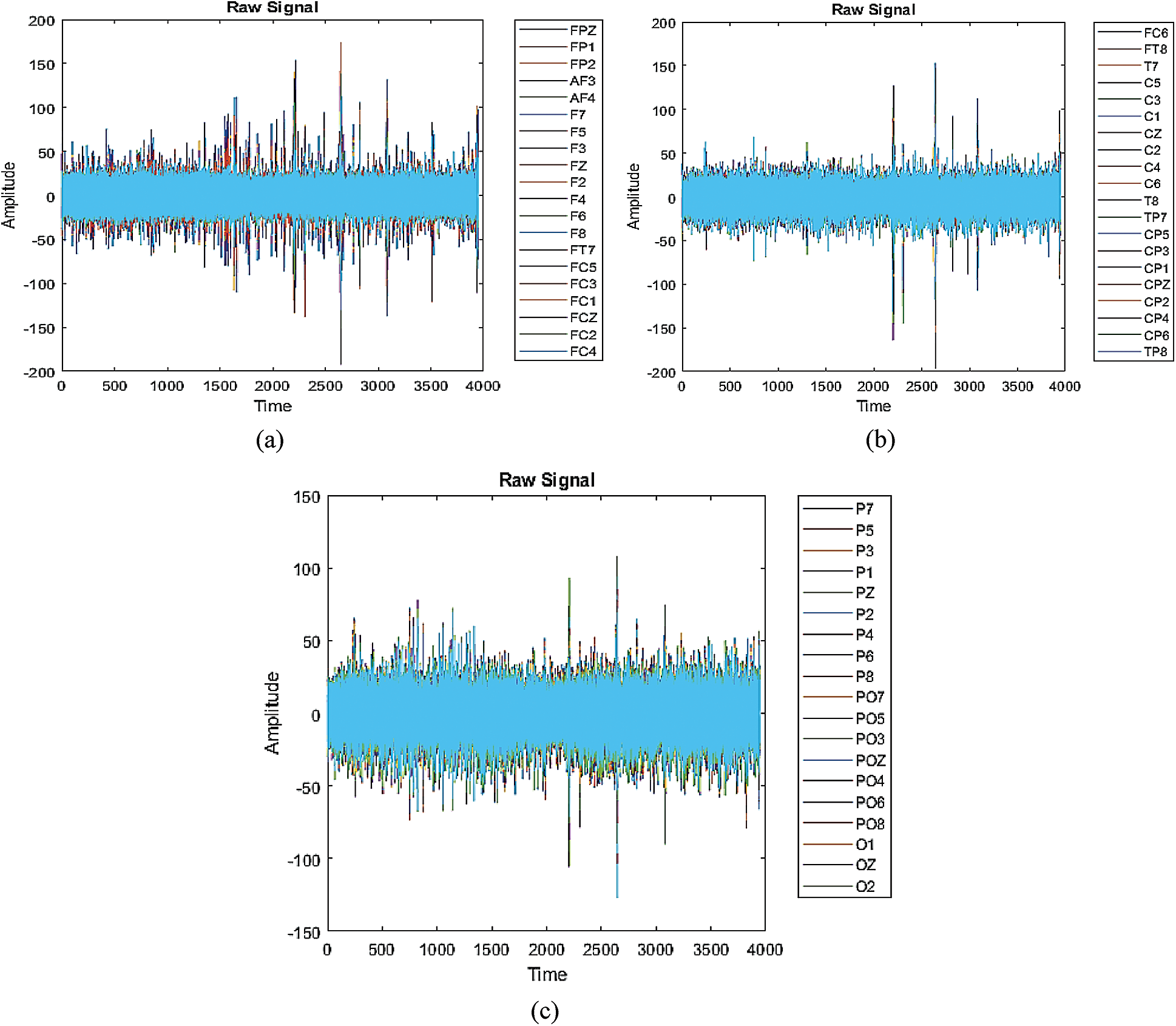
Figure 2: Raw signal combined all trials. (a) Raw signals part 1 (b) raw signals part 2 (c) raw signals part3
2) Pre-processing
A 64-channel electroencephalogram (EEG) amplifier from Neuroscan was used to record data for all the subjects. The left mastoid was used as a reference, and the ground was used for the right one. For the recording of signals, there were 60 electrodes based on EEG that were positioned on the surface of the brain. The EEG signals captured were tested at 250 Hz. For removing noise due to the power line after filtering the signals at 50 Hz, a notch filter was used. The raw and filtered signals are shown in Fig. 3. The raw signal for the single electrode is shown in Fig. 3d and after applying the filter the resultant signal is shown in Fig. 3e.
The trials with artifacts were also included. Trig value in data tells about the start of each trial and Class Label gave information about the classes that were labeled as “1” as the left hand, “2” as the right hand, “3” as the tongue, and “4” as the foot. For our work data of the first three seconds is removed and data from time
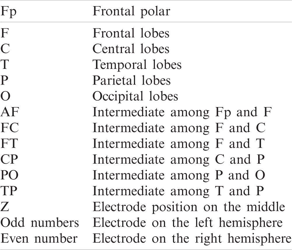
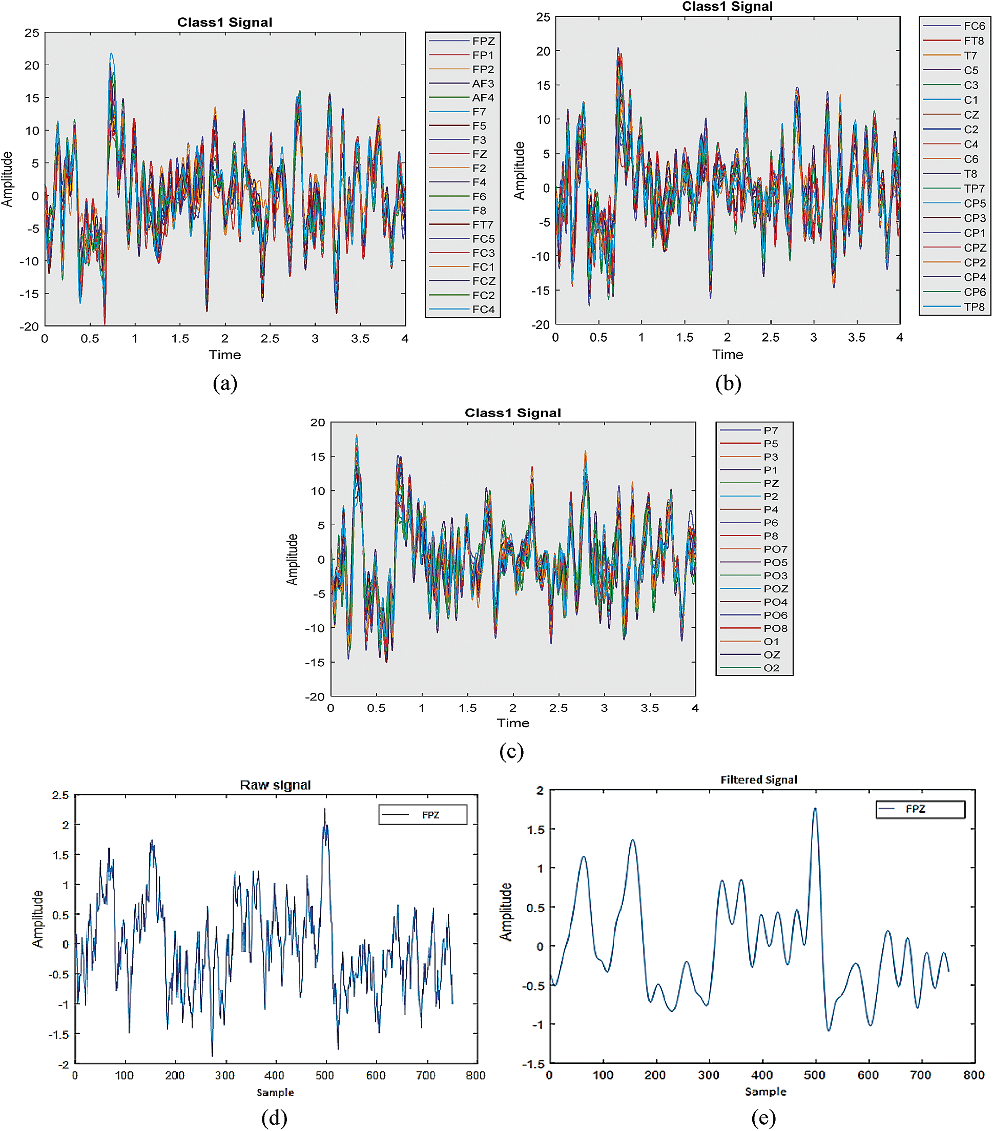
Figure 3: Raw and Filtered Signals. (a) Single class trial part 1 (b) single class trial part 2 (c) single class trial part 3 (d) raw signal (e) filtered signal
3.1.2 BCI Competition IV, Dataset IIa
1) Paradigm
The paradigm of BCI Competition IV, dataset IIa used in this work is shown in Fig. 4. At the time
The data was collected from 9 subjects. There were four different classes labeled as ‘1’, ‘2’, ‘3’, and ‘4’. Class 1 for left-hand motor imagery, 2 for the right hand, 3 for feet, and 4 for tongue imagery. The artifact data is included in this work. Two sessions were held on different days for experimenting and there was a total of 6 runs in each of the sessions. Each run was separated by a short break. There were 48 trials in each run. Overall, there was 288 trial per session for each subject. For each class there were 72 trials, for training and evaluation, there were 288 trials for each subject. The raw data including all the runs along with short breaks for a single subject is shown in Fig. 4a. Each color represents the channel or electrode placed on the scalp. There were a total of 25 channels. Since we were working on EEG signals only the first 22 channels were selected. Fig. 4b shown single class motor imagery activity collected from time
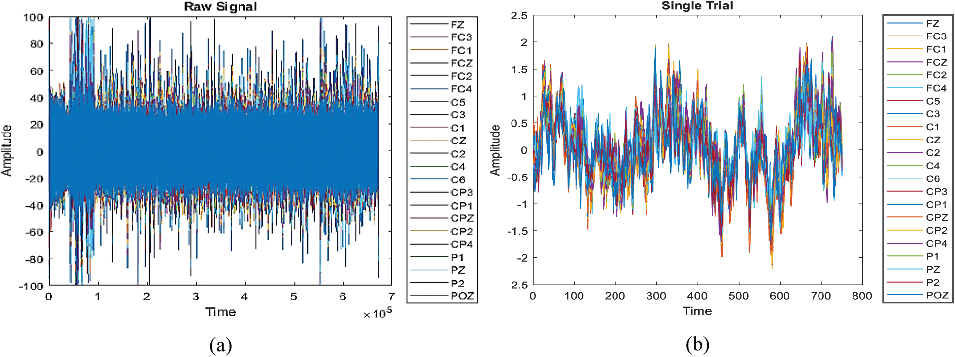
Figure 4: Raw data. (a) Raw data of all trials (b) single trial data
2) Pre-processing
The experiment consisted of 9 subjects and the data set comprises 25 channels. Among those 25, there were 22 electroencephalograms (EEG) channels and 3 monopolar electrooculograms (EOG) channels. For reference, the left mastoid was used while the right one was for a ground purpose. For the recording of signals 22 EEG and 3 EOG, the electrodes were positioned on the brain’s surface and the sampling rate of captured signals was 250 Hz. For the removal of noise due to the powerline the notch filter was applied at 50Hz. Afterward, a bandpass filter was applied at cuff-off frequencies of 0.5 and 100 Hz. In this work, only data samples were used from 22 EEG channels.
The raw dataset was given in the format of GDF and for the loading of the data BioiSig, toolbox functions were used [30]. After on onset of cross fixation we extracted the data samples in a time interval from 3 to 6 s. Each collected sample was further segmented at a rate of 50 Hz. The data set is used with a window size of 1, 2, and 3 s to check the accuracy results of the classifier. Separate datasets were provided for training and testing.
The methodology that was adopted for this work is shown in Fig. 5. Data acquisition and data preprocessing have been discussed in the previous section. After gathering the preprocessed signals the next step is choosing the architecture. In this work, we have used ANN and LSTM architecture for the classification of motor imagery datasets. After selecting the appropriate architecture we trained the model. Then the test datasets were passes to the trained model to get the accuracy results for both the architectures. The architectures used in this work and the accuracy results are discussed in later sections.
In deep neural networks, several layers of neurons are arranged over each other. The performance of the network can be improved by adding hidden layers to the network [31]. As the number of layers increases the complexity of the network increases. The major advantage of deep learning algorithms is there is no need to manually extract features which is a challenging task in the machine learning method. We just have to feed the dataset to the network it automatically learns the features. In this work we use two methods; we worked on ANN and RNN with LSTM architecture.
3.3.1 Artificial Neural Network (ANN)
The ANN is a feed-forward network consisted of various layers [32]. Backpropagation is used to update the weights. The architecture comprises 10 layers. There are the following different types of layers in this architecture: an input layer, a ReLU layer, and fully connected dense layers. The network has an input layer that is then converted to a one-dimensional array and connected to eight fully connected dense hidden layers. In each hidden layer, the neurons depend on the inputs of the input layer. In these layers, input and output are linked through a learnable weight. Each connected layer is also passed through non-linear activation functions such as ReLU. The final layer typically has the same number of nodes as the number of classes the input data must be classified into. The last layer’s activation function is chosen very carefully and is usually different from previous fully connected layers. One of the most commonly used layers is SoftMax, which normalizes the results between 0 and 1 based on the probability of each class. Typically, neural networks are updates by stochastic gradient descent. The training algorithm was chosen as stochastic gradient descent (SGD). The size of the batch was set to 64 and the layers. All the hyperparameters like the number of neurons, learning rate, weights, optimizer, and batch size were chosen empirically with repeated network training for achieving optimized accuracy results. The accuracy results are greatly affected by the selection of hyper-parameters [33] and the hyper-parameters used in this study are shown in Tab. 2. It is convenient to adjust the training iterations freely [34]. Apart from hyperparameters mentioned, Bayesian optimization can also be utilized to improve the overall performance of the system. In our work, the model was trained on 150 epochs. For this specific study, the learning rate selected was 0.01. A larger learning rate causes divergence in the network inversely, the smaller the learning rate network convergence will be slow. For the performance analysis metrics, the mean classification accuracy for different window sizes on the subjects was considered. A deep learning approach was used as we do not need to manually extract features for the motor imagery signals. The network learns to extract features while training and we just have to feed the signals dataset to the network. As in CNN and RNN, more data inputs or features are required to achieve the better accuracy as compared to ANN. However, the proposed method has employed deep learning approach using ANN as it does not require to extract many features. The architecture used in this study is shown in Fig. 6.
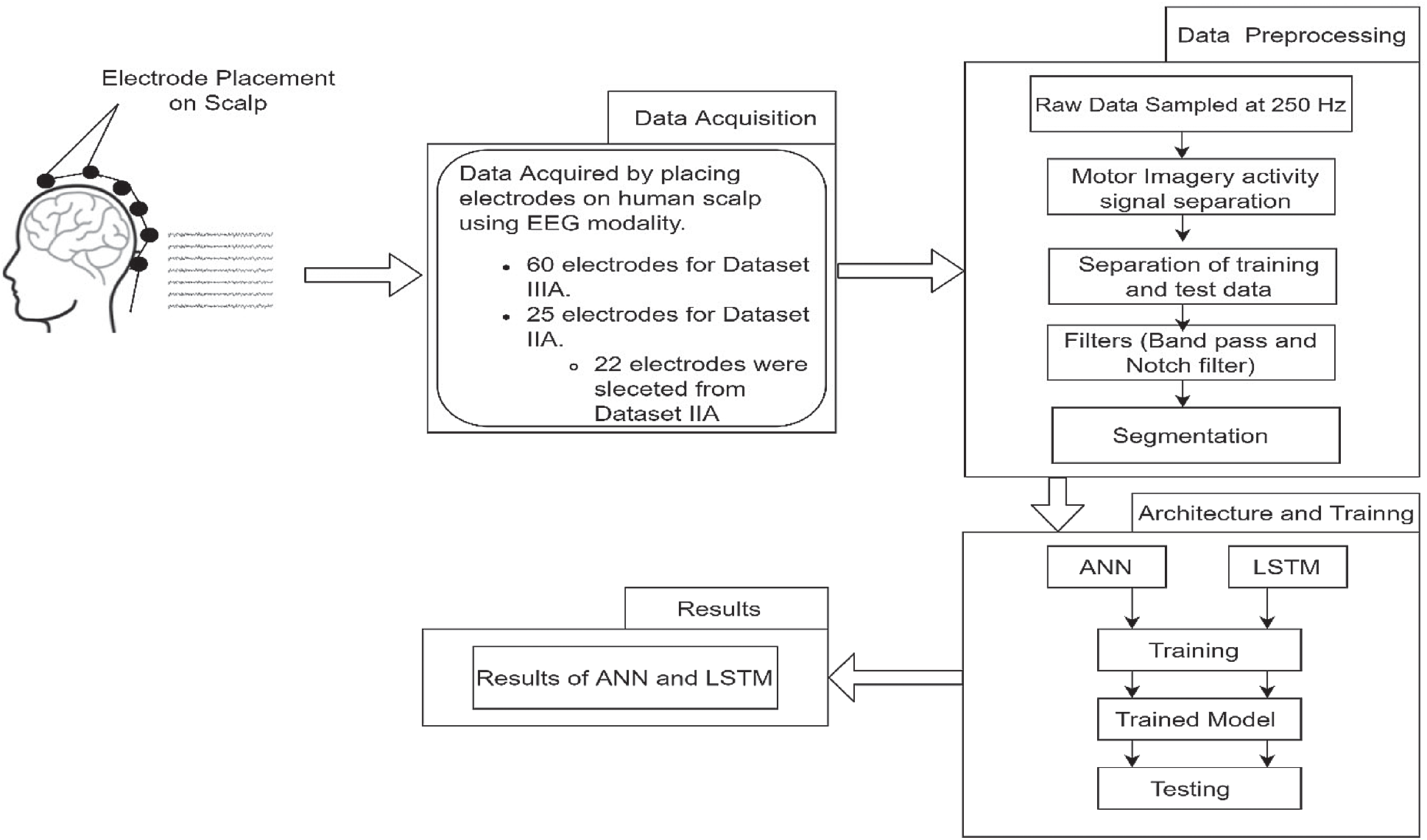
Figure 5: Flow chart for adopted methodology
3.3.2 Long Short-Term Memory (LSTM)
The other Architecture that we are using for exploring the classification of EEG signals is long short-term memory (LSTM). It is one of the types of recurrent neural networks. The Recurrent Neural networks were initially represented by Schmidhuber’s research group [35,36]. According to previous studies LSTM networks provide the best results for time series data classification, and it also provides better results as compared to conventional neural networks [37,38]. It works on the principle of saving the output of a layer and feeding that output to the next input layer which helps in the prediction of the layer’s outcome. LSTM is one of the types of RNN which can learn from observation which is an advantage of LSTM over other RNN types and neural networks. The major of LSTM is the cell state which can be changed i.e., can be deleted or added. [39] There are three gates in LSTM i.e., forget gate, input gate, and output gate. The purpose of forget gate is to delete the information from the cell. The input gate’s purpose is to check which information is to be updated. Whereas, the output gate gives the final output of the network [40].
Table 2: Parameters to train ANN
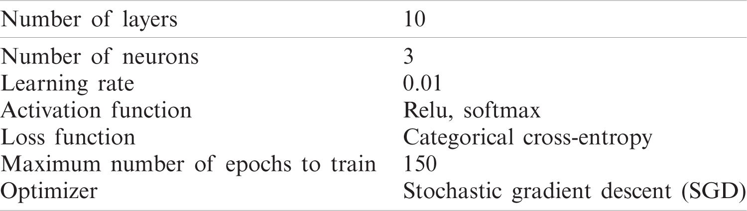
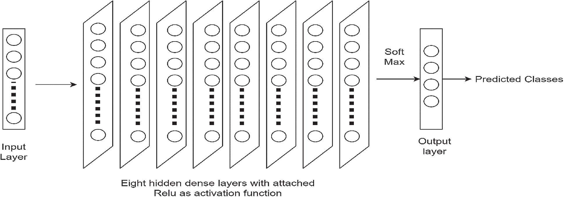
Figure 6: Proposed ANN architecture
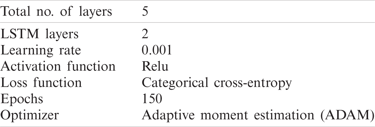
There are the following different types of layers in this architecture: an input layer, lstm layer, ReLU layer, and the fully connected dense layers. The proposed architecture is shown in Fig. 7. Pre-processed samples are given as input to the LSTM layer. LSTM layer is connected to the hidden layers which include a flatten layer and dense layer. After the dense layer, the Relu layer is added. Followed by Relu is the output layer which has softmax as the activation function. The output layer has 4 nodes as there are four classes in our datasets. The optimizer used in LSTM was Adam. For the performance analysis metrics, the mean classification accuracy for different window sizes on the subjects was considered. The parameters used in this study for LSTM architecture are given in Tab. 3. All the hyper-parameters were selected empirically after training the network. The aim was to achieve maximum accuracy results.
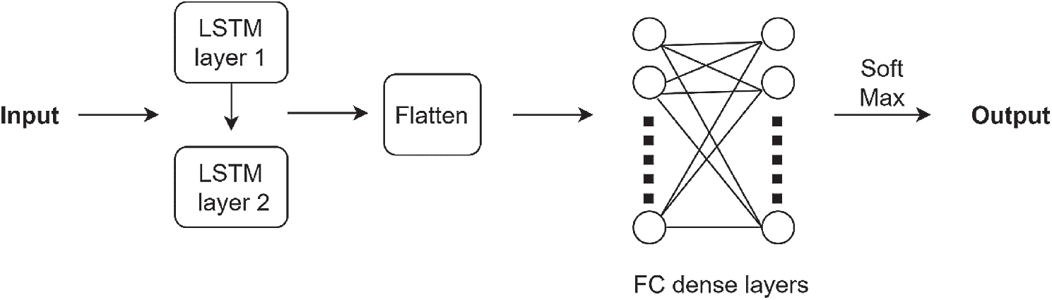
Figure 7: Proposed LSTM architecture
Table 3: Parameters to train LSTM
The results of the different classifiers used in this study are presented in this section. Two different deep learning classification algorithms were tested on both datasets IIIa, IIa, and for all the subjects of both the datasets the accuracy, results are listed in the table. Tab. 4 presents the classification results ANN and LSTM using BCI competition III, dataset IIIa. Whereas, Tab. 5 presents the classification results ANN and LSTM using BCI competition IV, dataset IIa.
From the results tables, we have concentrated on two things: the first comparison of both the architectures used in the study for both datasets and secondly, accuracy results using different window sizes. For BCI competition III, dataset IIIa if we compare the results of ANN with LSTM, the LSTM Architecture gave higher accuracy results. Four different window sizes of 1, 2, 3, and 4 s were used for dataset IIIa and the results in Tab. 4 prove that if we increase the window size classification accuracy improves inversely, decreasing the window size from 4 to 3 s, 2 s, or 1 s the accuracy decreases. LSTM shows more classification accuracy in comparison to the ANN. The maximum accuracy achieved on dataset IIIa using ANN is 94.7% and for LSTM the maximum accuracy on 4 s window size is 96.2%.
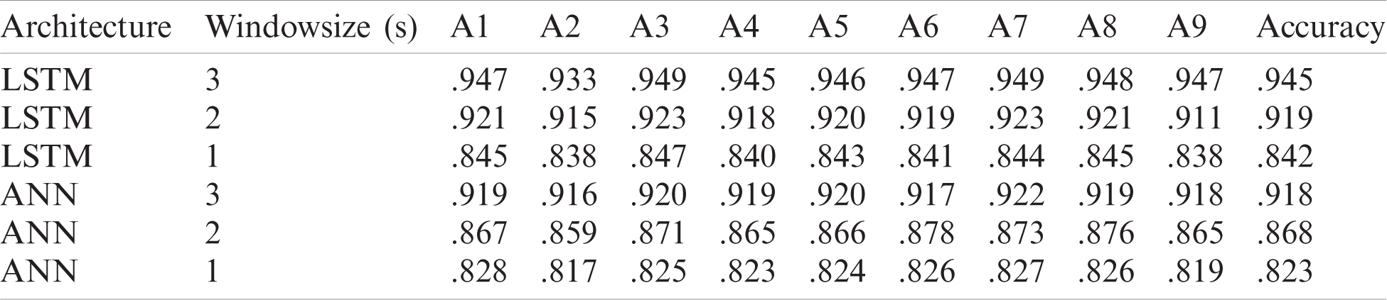
For dataset IIa different window sizes of 1, 2 s and 3 s was used and the results in the table show that accuracy results are higher at 3 s window size. The ANN architecture gave a maximum accuracy of 91.8% and for LSTM maximum achieved accuracy is 94.5% at 3 s window size. The deep learning methods outperform significantly. They can give better results without feature extraction as the network itself learned the desired features automatically.
Table 4: Classification accuracies for dataset IIIa using different window sizes
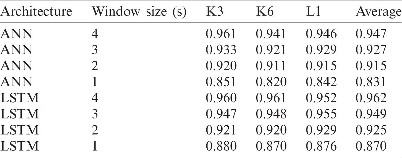
Table 5: Classification accuracies for dataset IIa using different window sizes
Accuracy and loss plots for the datasets for ANN are shown in Figs. 8a, 8b, and for LSTM in Figs. 9a and 9b. Accuracy plots show that’s as the number of epochs increases the training and test accuracy increases and after a certain number of epochs it increases to its maximum value. The green color shows the training accuracy while blue shows the test accuracy. For loss plots in Figs. 8b and 9b loss value decrease as the training, iterations are increasing, and after a certain epoch, loss reaches its minimum value.
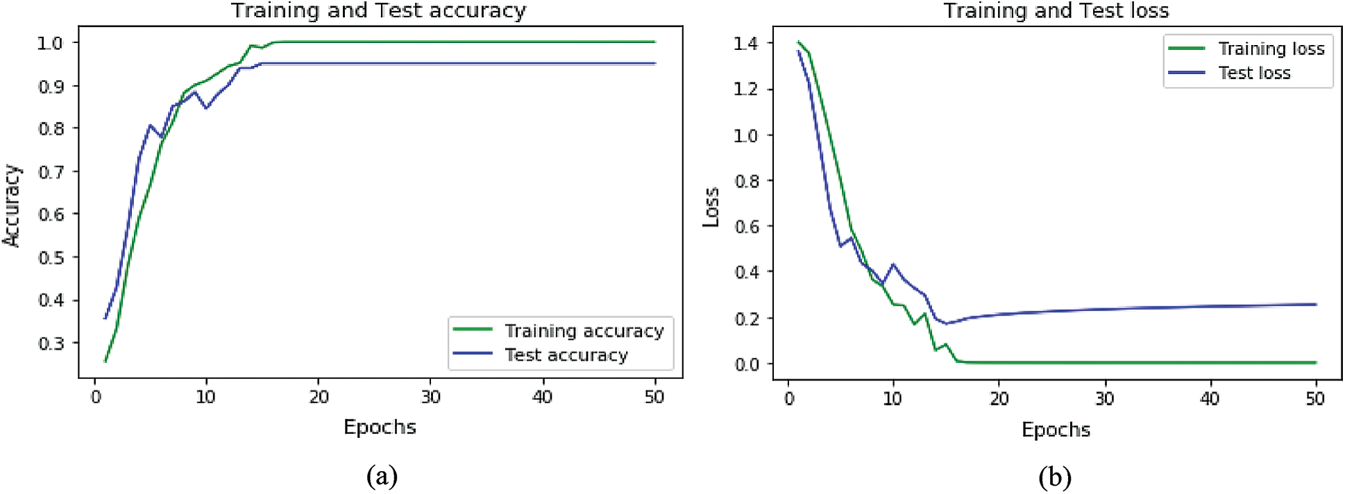
Figure 8: Accuracy and loss graphs for ANN: (a) Accuracy graph for ANN (b) loss graph for ANN
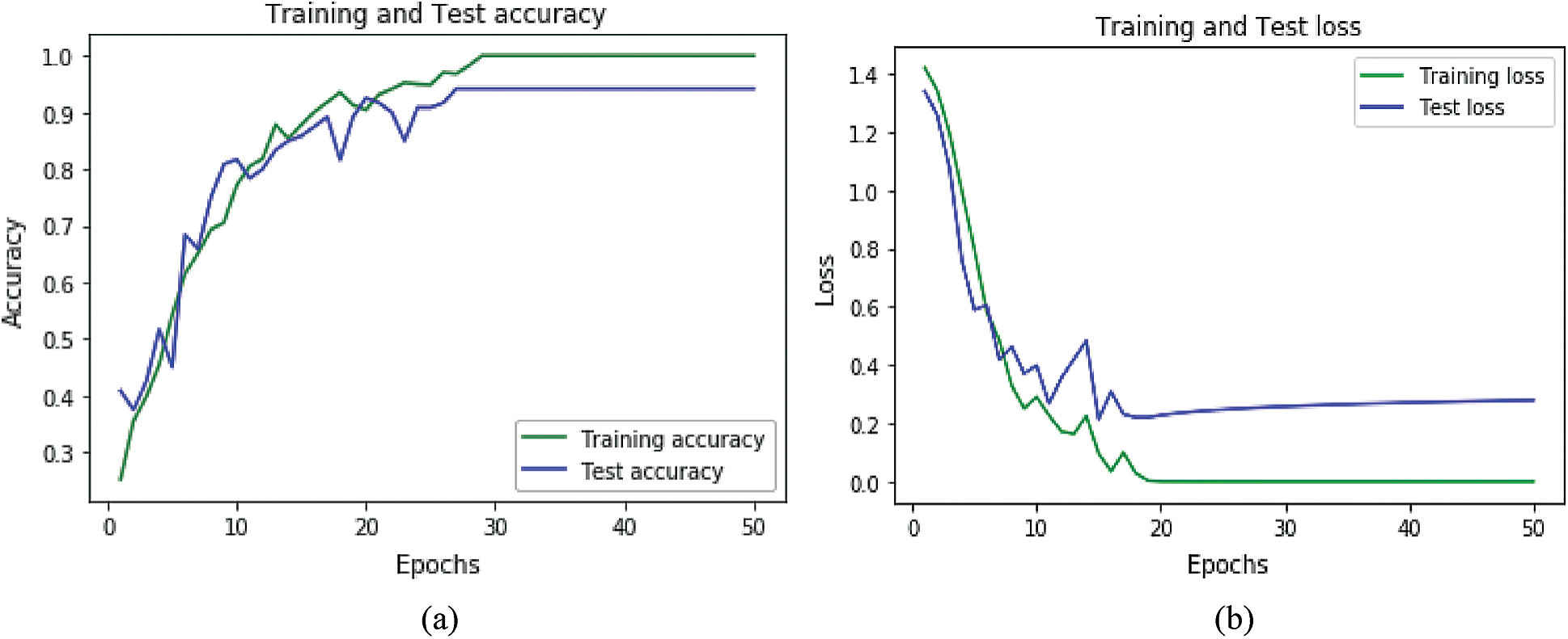
Figure 9: Accuracy and loss graphs for LSTM: (a) Accuracy graph for LSTM (b) accuracy and loss graph for LSTM
We have explored the classification algorithms for four-class motor imagery-based EEG signals. The target of the work was to critically analyze and assess the efficiency of the machine and deep learning technique. Two publicly available motor imagery datasets comprising of a total of 13 subjects and 4 classes were used to train, validate, and test the deep learning models. The datasets were in the form of electrical signals, before training the model, the data was pre-processed. ANN and LSTM, a machine and deep learning classifier, respectively have been used to classify waste collections. Classification accuracies have been reported to test the performance of both the classifiers. The effect of choosing different window sizes is also evaluated. The results show that increasing the window size has a better effect on classification accuracy.
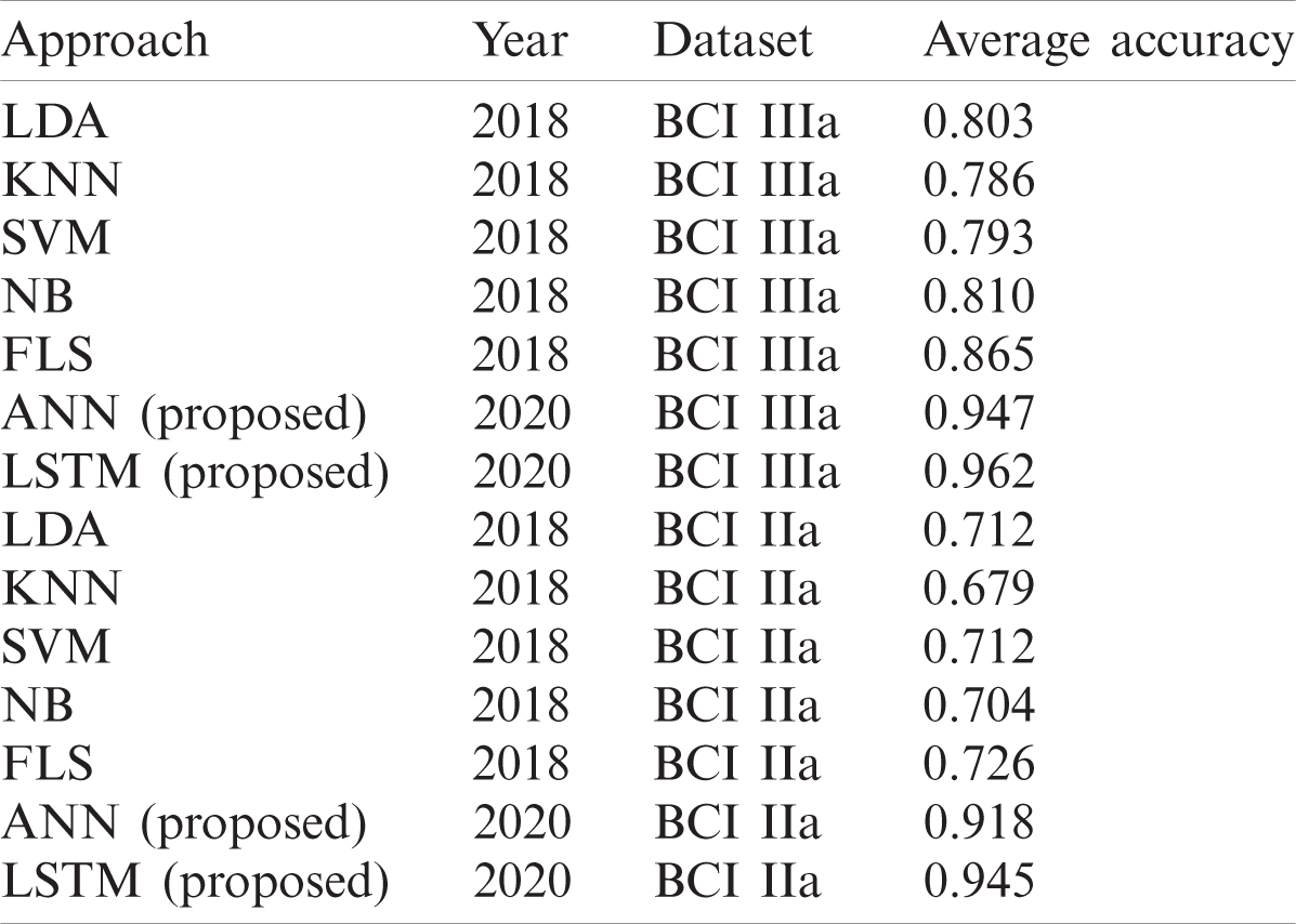
For dataset IIIa, BCI competition III a comparison Tab. 6 is shown below according to a study [41]. For accuracy results for this dataset, our proposed LSTM gives the performance having an accuracy of 0.962. The second best method is ANN that gives an accuracy of 0.947. The algorithm with the least accuracy is LDA. For dataset IIa, BCI competition IV the results are similar to the previous dataset, LSTM attains the performance with an average accuracy rate of 0.945 and ANN classifier with an average accuracy of 0.918 whereas, KNN gives the lowest average accuracy of 0.679 percent.
Apart from manual feature extraction, machine learning algorithms tend to generalize the complicated data patterns and therefore resulted in poor performance when we increase the number of classes. Most of the previous studies worked on binary classes using traditional machine learning algorithms. But when we discuss the classification of two mental tasks the achieved accuracy was 87% using the conventional ML algorithm SVM [42]. In the same study, 87.2% accuracy was achieved using SVM on two different brain signals.
The results showed that the LSTM outperforms ANN in classifying the datasets. For dataset IIIa, the accuracy results of ANN ranges from 83.0 to 94.7% for four different window sizes, and for LSTM it ranges from 87.1 to 96.2% for a window size of 1 to 4 s. For dataset IIa, the accuracy for ANN ranges from 82.3 to 91.8%, and for LSTM it ranges from 84.2% to 94.5% for a window size of 1 to 3 s.
Table 6: Comparison of deep learning algorithms on BCI competition III, dataset IIIa, and BCI competition IV, dataset IIa
In future work, increasing the dataset may have better effects on accuracy. Similarly, we can focus on developing efficient algorithms that can work for noisy signals.
Acknowledgement: This research work was supported by National University of Sciences and Technology, Pakistan.
Funding Statement: This research was financially supported in part by the Ministry of Trade, Industry and Energy (MOTIE) and Korea Institute for Advancement of Technology (KIAT) through the International Cooperative R&D program. (Project No. P0016038) and in part by the MSIT (Ministry of Science and ICT), Korea, under the ITRC (Information Technology Research Center) support program (IITP-2021-2016-0-00312) supervised by the IITP (Institute for Information & communications Technology Planning & Evaluation).
Conflicts of Interest: The authors declare that they have no conflicts of interest to report regarding the present study.
1. L. F. Nicolas-Alonso and J. Gomez-Gil, “Brain-computer interfaces, a review,” Sensors, vol. 12, no. 2, pp. 1211–1279, 2012. [Google Scholar]
2. C. G. Coogan and H. Bin, “Brain-computer interface control in a virtual reality environment and applications for the internet of things,” IEEE Access, vol. 6, pp. 10840–10849, 2018. [Google Scholar]
3. R. A. Ramadan and A. V. Vasilakos, “Brain-computer interface: Control signals review,” Neurocomputing, vol. 223, no. 1, pp. 26–44, 2017. [Google Scholar]
4. J. van Erp, F. Lotte and M. Tangermann, “Brain-computer no interfaces: Beyond medical applications,” Computer, vol. 45, no. 4, pp. 26–34, 2012. [Google Scholar]
5. G. Z. Yang, J. Bellingham, P. E. Dupont, P. Fischer, L. Floridi et al., “The grand challenges of science robotics,” Sci. Robot, vol. 3, no. 14, pp. eaar7650, 2018. [Google Scholar]
6. M. Ahn, M. Lee, J. Choi and S. C. Jun, “A review of brain-computer interface games and an opinion survey from researchers, developers, and users,” Sensors, vol. 14, no. 8, pp. 14601–14633, 2014. [Google Scholar]
7. S. N. Abdulkadesr, A. Aria and M.-S. M. Mostafa, “Brain-computer interfacing: Applications and challenges,” Egyptian Informatics Journal, vol. 16, no. 2, pp. 213–230, 2015. [Google Scholar]
8. J. Thomas, T. Maszczyk, N. Sinha, T. Kluge and J. Dauwels, “Deep learning-based classification for brain-computer interfaces,” in 2017 IEEE Int. Conf. on System, Man, and Cybernetics, Banff, AB, pp. 234– 239, 2017. [Google Scholar]
9. M. A. Hearst, S. T. Dumais, E. Osuna, J. Platt and B. Scholkopf, “Support vector machines,” IEEE Intelligent Systems and Their Applications, vol. 13, no. 4, pp. 18–28, 1998. [Google Scholar]
10. H. Ramchoun, M. Amine, J. Idrissi, Y. Ghanou and M. Ettaouil, “Multilayer perception: Architecture optimization and training,” IJIMAL, vol. 4, no. 1, pp. 26–30, 2016. [Google Scholar]
11. D. F. Morrison, “Multivariate analysis, overview,” 2005. [Online]. Available: https://onlinelibrary.wiley.com/doi/abs/10.1002/0470011815.b2a13047. [Google Scholar]
12. X. An, D. Kuang, X. Guo, Y. Zhao and L. He, “A deep learning method for classification of EEG data based on motor imagery,” in D. S. Huang, D. S. Huang, K. Han, M. Gromiha (eds.Intelligent Computing in Bioinformatics, vol. 8590, 2014. [Google Scholar]
13. T. Reddy, S. Bhattacharya, P. K. Maddikunta, S. Hakak, W. Z. Khan et al., “Antlion re-sampling based deep neural network model for classification of imbalanced multimodal stroke dataset,” Multimed Tools Appl., vol. 9, pp. 1–25, 2020. [Google Scholar]
14. C. Iwendi, S. Khan, J. H. Anajemba, A. K. Bashir and F. Noor, “Realizing an efficient IoMT-assisted patient diet recommendation system through machine learning model,” IEEE Access, vol. 8, pp. 28462–28474, 2020. [Google Scholar]
15. J. Yang, H. Singh and E. L. Hines, “Channel selection and classification of electroencephalogram signals: An artificial neural network and genetic algorithm-based approach,” Artificial Intelligence in Medicine, vol. 55, no. 2, pp. 117–126, 2012. [Google Scholar]
16. J. M. Aguilar, J. Castillo and D. Elias, “EEG signals processing based on fractal dimension features and classified by neural network and support vector machine in motor imagery for a BCI,” VI Latin American Congress on Biomedical Engineering, vol. 49, pp. 615–618, 2014. [Google Scholar]
17. M. Serdar Bascil, A. Y. Tenseli and F. Temurtas, “Multichannel EEG signal feature extraction and pattern recognition on horizontal mental imagination task of 1-D cursor movement for the brain-computer interface,” Australasian Physical & Engineering Science in Medicine, vol. 38, no. 2, pp. 229–223, 2015. [Google Scholar]
18. R. J. Williams and D. Zipser, “A learning algorithm for continually running fully recurrent neural networks,” Neural Computation, vol. 1, no. 2, pp. 270–280, 1989. [Google Scholar]
19. S. Hochreiter and J. Schmidhuber, “Long short-term memory,” Neural Computation, vol. 9, no. 8, pp. 1735–1780, 1997. [Google Scholar]
20. J. Dihong, Y. Lu, M. A. Yu and W. Yuanyuan, “Robust sleep stage classification with single-channel EEG signals using multimodal decomposition and HMM-based refinement,” Expert Systems with Applications, vol. 121, pp. 188–203, 2019. [Google Scholar]
21. D. Ravi, “Deep Learning for health Informatics,” IEEE J. Biomed. Heal. Informatics, vol. 21, no. 1, pp. 4–21, 2017. [Google Scholar]
22. M. Srirangan, R. K. Tripathy and R. B. Pachori, “Time-frequency domain deep convolutional neural network for the classification of focal and non-focal EEG signals,” IEEE Sensors Journal, vol. 20, no. 6, pp. 3078–3086, 2019. [Google Scholar]
23. E. C. Djamal, M. Y. Abdullah and F. Renaldi, “Brain computer interface game controlling using fast fourier transform and learning vector quantization,” Journal of Telecommunication, Electronic and Computer Engineering, vol. 9, no. 2–5, pp. 71–74, 2017. [Google Scholar]
24. J. Liu, Y. Cheng and W. Zhang, “Deep learning EEG response representation for brain computer interface,” in Chinese Control Conf., pp. 3518–3523, 2015. [Google Scholar]
25. E. C. Djamal and R. D. Putra, “Brain-computer interface of focus and motor imagery using wavelet and recurrent neural networks,” TELKOMNIKA Telecommunication Computing Electronics and Control, vol. 18, no. 4, pp. 2748–2756, 2020. [Google Scholar]
26. F. M. Garcia-Moreno, M. Bermudez-Edo, M. J. Rodríguez-Fórtiz and J. L. Garrido, “A CNN-LSTM deep learning classifier for motor imagery EEG detection using a low-invasive and low-cost BCI headband,” in 16th Int. Conf. on Intelligent Environments, Madrid, Spain, pp. 84–91, 2020. [Google Scholar]
27. B. Blankertz, “The BCL competition III: Validating alternative approach to actual BCI problems,” IEEE Trans. Neural Syst Rehabil. Eng, vol. 14, no. 2, pp. 153–159, 2006. [Google Scholar]
28. M. Tangemment, “Review of the BCI competition IV,” Frontiers Neurosci, vol. 6, pp. 55, 2012. [Google Scholar]
29. K. K. Ang, Z. Y. Chin, C. Wang, C. Guan and H. Zhang, “Filter bank common spatial pattern algorithm on BCI competition IV datasets 2a and 2b,” Frontiers Neurosci, vol. 6, pp. 39, 2012. [Google Scholar]
30. L. F. Nicolas-Alonso and J. Gomez-Gil, “Brain-computer interface, a review,” Sensors, vol. 12, no. 2, pp. 1211–1279, 2012. [Google Scholar]
31. D. S. Kermany, M. Goldbaum, W. Cai, C. Valentim, H. Liang et al., “Identifying medical diagnoses and treatable diseases by image-based deep learning,” Cell, vol. 172, no. 5, pp. 1122–1131, 2018. [Google Scholar]
32. F. Lotte, L. Bougrain, A. Cichocki, M. Clerc, M. Congedo et al., “A review of a classification algorithm for EEG-based brain-computer interface: A 10-year update,” J. Neural Eng., vol. 15, no. 3, pp. 31005, 2018. [Google Scholar]
33. L. N. Smith, “Cyclical learning rates for training neural networks,” in IEEE Winter Conf. on the Application of Computer Vision, Santa Rosa, CA, pp. 464–472, 2017. [Google Scholar]
34. Y. Bengio, “Practical recommendation for gradient-based training of deep architecture,” in G. Montavon, G. B. Orr, K. R. Muller (eds.Neural Networks: Tricks of the Trade. Lecture Notes in Computer Science, vol. 7700. Berlin, Heidelberg: Springer, 2012. [Google Scholar]
35. J. Schmidhuber and S. Hochreiter, “Long short-term memory,” Neural Computation, vol. 9, no. 8, pp. 1735–1780, 1997. [Google Scholar]
36. L. C. Schudlo and T. Chau, “Dynamic topographical pattern classification of multichannel prefrontal NIRS signals,” II: Online Differentiation of Mental Arithmetic and Rest. J Neural Eng., vol. 11, pp. 1741–2560, 2013. [Google Scholar]
37. A. Graves, M. Liwick, S. Fernandez, R. Bertolami, H. Bunke et al., “A Novel connection systems for unconstrained handwriting recognition,” IEEE Trans. Part. Anal. Mach. Intel, vol. 31, no. 5, pp. 855–868, 2009. [Google Scholar]
38. A. Graves, A. R. Mohamed and G. Hinton, “Speech recognition with deep recurrent neural networks,” in ICASSP IEEE Int. Conf. in Acoustics, Speech and Signals Processing, Vancouver, BC, pp. 6645–6649, 2013. [Google Scholar]
39. K. Greff, R. K. Srivastava, J. Koutunik, B. R. Steunebrink and J. Schmidhuber, “LSTM: A search space odyssey,” IEEE Trans. Neural Network. Learn. Syst, vol. 28, pp. 2222–2232, 2016. [Google Scholar]
40. Y. Luan and S. Lin, “Research on text classification based on CNN and LSTM,” in IEEE Int. Conf. on Artificial Intelligence and Computer Application, Dalian, pp. 352–355, 2019. [Google Scholar]
41. T. Nguyen, I. Hettiarachchi, A. Khatami, L. Gordon-Brown, C. P. Lim et al., “Classification of multi-class BCI data by common spatial pattern and fuzzy Systems,” IEEE Access, vol. 6, pp. 27873–27884, 2018. [Google Scholar]
42. N. Naseer and K. S. Hong, “Classification of functional near-infrared spectroscopy signals corresponding to right-and left-wrist motor imagery for development of a brain-computer interface,” Neurosci Letter, vol. 553, pp. 84–89, 2013. [Google Scholar]
 | This work is licensed under a Creative Commons Attribution 4.0 International License, which permits unrestricted use, distribution, and reproduction in any medium, provided the original work is properly cited. |