Computers, Materials & Continua DOI:10.32604/cmc.2021.017086
Article

Data Matching of Solar Images Super-Resolution Based on Deep Learning

Liu Xiangchun1, Chen Zhan1, Song Wei*,1,2,3, Li Fenglei1 and Yang Yanxing4

1School of Information Engineering, Minzu University of China, Beijing, 100081, China
2National Language Resource Monitoring and Research Center of Minority Languages, Minzu University of China, Beijing, 100081, China
3CAS Key Laboratory of Solar Activity, National Astronomical Observatories, Beijing, 100101, China
4Department of Physics, New Jersey Institute of Technology, Newark, New Jersey, 07102-1982, USA
*Corresponding Author: Song Wei. Email: songwei@muc.edu.cn
Received: 20 January 2021; Accepted: 23 March 2021

Abstract: The images captured by different observation station have different resolutions. The Helioseismic and Magnetic Imager (HMI: a part of the NASA Solar Dynamics Observatory (SDO) has low-precision but wide coverage. And the Goode Solar Telescope (GST, formerly known as the New Solar Telescope) at Big Bear Solar Observatory (BBSO) solar images has high precision but small coverage. The super-resolution can make the captured images become clearer, so it is wildly used in solar image processing. The traditional super-resolution methods, such as interpolation, often use single image’s feature to improve the image’s quality. The methods based on deep learning-based super-resolution image reconstruction algorithms have better quality, but small-scale features often become ambiguous. To solve this problem, a transitional amplification network structure is proposed. The network can use the two types images relationship to make the images clear. By adding a transition image with almost no difference between the source image and the target image, the transitional amplification training procedure includes three parts: transition image acquisition, transition network training with source images and transition images, and amplification network training with transition images and target images. In addition, the traditional evaluation indicators based on structural similarity (SSIM) and peak signal-to-noise ratio (PSNR) calculate the difference in pixel values and perform poorly in cross-type image reconstruction. The method based on feature matching can effectively evaluate the similarity and clarity of features. The experimental results show that the quality index of the reconstructed image is consistent with the visual effect.

Keywords: Super resolution; transition amplification; transfer learning

1  Introduction

The study of solar activity has always been a key issue in the field of astronomy. Obtaining high-precision solar images is the basis to study the Sun. We hope to train a super-resolution network from the Helioseismic and Magnetic Imager (HMI: a part of the NASA Solar Dynamics Observatory (SDO) solar images with low-precision but wide coverage to Goode Solar Telescope (GST, formerly known as the New Solar Telescope) at Big Bear Solar Observatory (BBSO) solar images with high precision but small coverage. The HMI covering the whole sun is captured by an orbiting satellite, which is not affected by the atmosphere. The shooting range includes the whole sun, and the precision is only 1 angular second per pixel (Fig. 1).

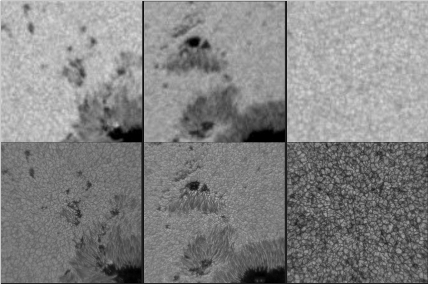
Figure 1: HMI, GST example diagrams, up: HMI, down: GST

GST solar images are captured by Big Bear Solar Observatory and the precision is 0.034 angular second per pixel, however, the shooting time and shooting range are easily affected by atmospheric turbulence and diurnal rhythm factors and the quantity is very small.

So far there has been super-resolution convolution neural network that puts the high-definition images and their down-sampling into the model to train the network. However, it is not feasible to replace the original GST down-sampling image with the HMI image directly when training from HMI images to GST images. For there is no strong feature alignment and similarity between HMI images and GST images comparing to the down-sampling GST images. And their feature offset and the feature detail deviations are very common. The receptive field of convolution operation is directly affected by the size of the convolution kernel. The reconstruction of these features will be difficult to be learned once the feature offset exceeds the radius of the convolution kernel. When building the HMI and GST images super-resolution network, the feature pre-alignment is needed to reduce the difference between the two types of images, and these tasks will be undertaken by the network training process if using the traditional deep-learning network, which will greatly increase the difficulty of training. To solve the problem, we try to add a transition image between a source image and a target image, which is an image of source image size and has a strong connection with both ends of the network. We call this network Transition-Amplification Network (TA Network), which inserts the transition image and divides the origin process into two sub-network parts (the image conversion and super-resolution), reducing the training difficulty of the two sub-networks greatly, avoiding designing or learning specific down-sampling methods to achieve pixel-level feature alignment from the GST image to the HMI image. The training of the network contains three parts. Firstly, it gets the transition images by reconstruction of high-definition and low-definition. Secondly, it maps from low-definition images to equal size transition images (transition network). Thirdly, it maps from transition images to target images (amplification network). In the test procedure, the low-definition images are reconstructed to the same size transition images from transition network and then reconstructed to the super-resolution images from amplification network. Finally, the super-resolution images close to the GST image definition is obtained.

2  Related Work

Before deep-learning is applied to solar image super-resolution, the traditional solar super-resolution reconstruction methods mainly include three types: speckle imaging (SI), multi-frame blind deconvolution (MFBD), and phase diversity (PD). SI need to count a group of short exposure images in advance and can be divided into frequency domain processing and spatial processing. The common methods of frequency-domain reconstruction include the Labeyrie’s method [1], Knox Thompson [2] (K-T) method, and speckle mask [3–5] method. The common methods of spatial reconstruction include simple displacement superposition [6–9], iterative displacement superposition [10], and correlation displacement superposition. Both the MFBD and PD methods use direct deconvolution to recover the target and use the optimization iterative method to get the target and wavefront phase for it is difficult to obtain the instantaneous point spread function of the sun accurately. The idea of blind deconvolution was first proposed by Stockham et al. [11] and then applied to blind deconvolution by Ayers et al. [12] and Davey et al. [13]. The phase difference method was proposed by Gonsalves et al. [14], which was only used in the field of wavefront detection at first, and then extended to the field of astronomical image restoration. Different from traditional ones, the deep-learning method based on supervised learning is almost divorced from prior knowledge, and the network optimizes the parameters in training to improve the reconstruction quality. This kind of network usually has a good effect, but the controllability is weak because gradient descent algorithm, the basic parameter learning mechanism, seeks the local optimal solution rather than the global one, which leads to the parameter learning affected by the initial value, the step length of a parameter change, the number of iterations of parameters, etc. And these factors often change with the learning progress of the network. In the process of parameter learning in a TA Network, the current parameters are reduced by reducing differences between input and target in the way of adding transition images, which means the length of the learning path is reduced for the original long learning path is split into two shorter paths, improving the controllability and stability of the separate training progress of the two networks.

3  The Data Matching Algorithm

3.1 Overall Framework

TA Network training includes three parts: transition image acquisition, transition network training with source images and transition images, and amplification network training with transition images and target images. The training quality of both the two networks has a great relationship with the transition images, so the acquisition of transition image is the core part of this framework. The model training process is in Fig. 2.

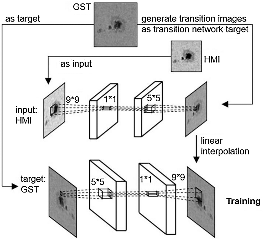
Figure 2: Model training process

3.2 Transition Images Acquisition

The method to get a transition image has a strong connection with the data set and application. Since HMI solar images and GST solar images have certain feature migration problems, and little similar work or data sets are available for reference.

We cannot retrain a supervised learning-based generation network. Considering the total training time, non-learning algorithms or network generation methods can be chosen. Unlike deep-learning methods [15–17], non-learning methods get functions and parameters determined with prior knowledge and generally remain unchanged with the using process. We use the classical scale-invariant Feature Transform [18] (SIFT) algorithm to extract potential feature points, and then extract potential matching feature pairs with the K-nearest Neighbor [19] (KNN) algorithm, and then use the Random Sample Consensus [20] (RANSAC) algorithm to remove the inconsistent feature pairs and calculates the homography matrix, transformation matrix, based on the rest extracted feature pairs. Finally, we multiply the GST images and the transformation matrix to obtain the transition images of the same size as the HMI image.

The network generation method does not need to prepare the transition image in advance but firstly takes the amplification network target image as the transition network target image. When the transition network training is completed, another group of test images with equal number are put into the transition network. The output images are the transition images. The advantage of this method is of wide adaptability for super-resolution, image conversion, and other fields. However, the transition images generated by this method are affected by many factors, including but not limited to the difference between the source images and the target images, the structure of the transition network, and the amount of data. Adjustments will be needed based on the application.

To verify the effect of adding a transition image, we use the basic Super-Resolution Convolutional Neural Network [21] (SRCNN) as the transition network and amplification network.

3.3 Transition Network

Different with the standard SRCNN, we need to learn a mapping network of equal end size. Since the output and input image size of the network are equal, we remove the bicubic interpolation amplification part in the front end of the network. The rest is the same as SRCNN, which includes three convolution layers. The convolution kernel sizes are 9×9, 1×1, and 5×5, and the number of output channels is 64, 32, 1. The dimensions, depth, and size of network input and output are consistent with the standard SRCNN.

3.4 Amplification Network

The amplification network is a standard SRCNN network. The transition image is interpolated as the network input to realize the super-resolution task from the transition image to the GST solar image. The role is the same as the traditional super-resolution network.

4  Relevant Algorithm

4.1 SRCNN

SRCNN (Fig. 3) is the first deep-learning network applied to super-resolution reconstruction. The network structure is simple relatively, including only three layers of neurons, without the common activation and pooling operations. SRCNN first enlarges the low-resolution image to the size of the target images by bicubic interpolation and then learns end-to-end mapping through three-layer convolution. The three-layer convolution structure is divided into three steps: patch extraction and representation, non-linear mapping, and reconstruction. The convolution kernels used by the three-layer neurons are 9×9, 1×1, and 5×5, The numbers of output features are 64, 32, 1 respectively.

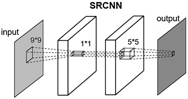
Figure 3: SRCNN structure

4.2 SIFT

SIFT feature extraction includes five parts-scale-space generation, scale detection, spatial extreme points, accurate location of extreme points, and assignment of direction parameters for each key-point, generation of key-point descriptors. The key-point descriptor is a 32-dimensional SIFT feature vector, which can be used for feature matching and etc.

4.3 RANSAC

RANSAC algorithm uses random sampling to remove the feature points that do not meet the consistency and derive the homography matrix. The algorithm effect is similar to Fig. 4.

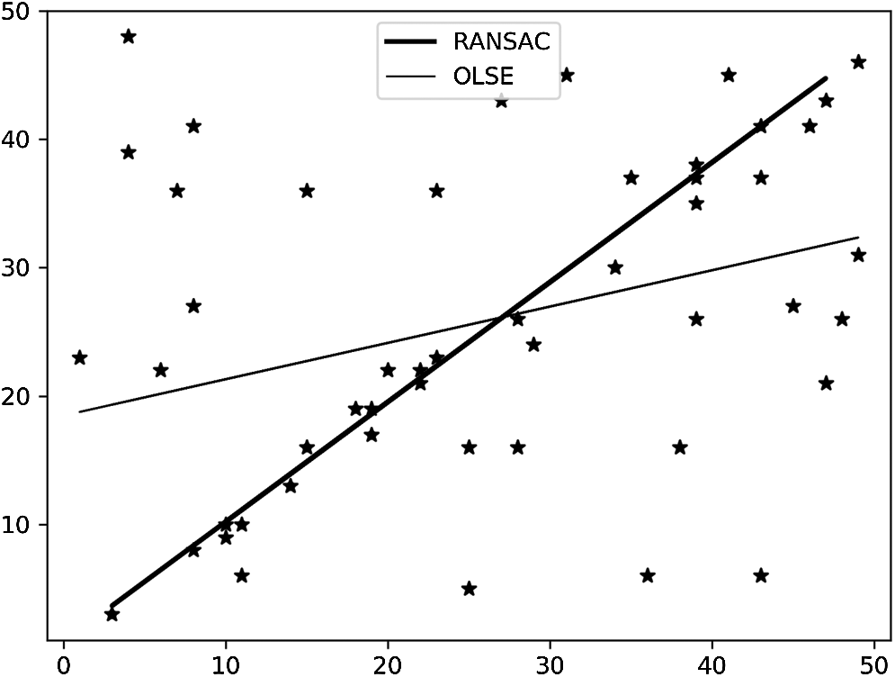
Figure 4: RANSAC, OLSE comparison diagram

Let n be the number of elements in the sample subset, p is the expected successful probability of the algorithm, w is the probability that the selected point belongs to the consistent set, and k is the number of iterations. The probability of all failures in k samples is:

p=(1-wn)k(1)

Namely:

k=log(1-p)log(1-wn)(2)

4.4 K-Nearest Neighbor Matching

After filtering out the feature points, we need to use the feature points matching algorithm to get feature pairs. Here we use K-Nearest Neighbor matching. When matching, we select k points from the source images that are most similar to the feature points of the target images. When the distance between the K feature points is large, the most similar point is selected as the matching point. Generally, K is selected to be 2. The correct matching needs to ensure that the distance between the K points is large.

5  Experimental Results and Analysis

This experiment runs on Python 3.6, Keras 2.3. The computing equipment is GTX1060 and i7-8750h processor. The data set includes HMI images of precision 1 angular second per pixel and GST images of precision 0.034 angular seconds per pixel. To convert the data into quadruple super-resolution standard data, we first rotate and segment the HMI image, and control the field of view to be equal to the GST image. Finally, the GST images are quadruply down-sampled, and we trim the edge of the GST and the HMI images. Finally, two hundred 114×114 HMI images and two hundred corresponding 456×456 GST images are obtained. At this time, the precision of the GST image is about 7-times than that of the HMI image.

To verify the necessity of the transition network, we controlled the same total training time and compared it with the SRCNN super-resolution network for HMI image to GST image. We discussed the limitations of evaluation indexes such as PSNR and SSIM in this field and proposed a new matching rate based on clarity and feature similarity as evaluation index.

In order to verify the effectiveness of the proposed method, three groups of experiments were carried out. Experiment 1: TA Network with SIFT transition images. Control two sub-networks with the same epoch. The training data is 50 groups of pictures, each group of the pictures includes a 114×114 fuzzy HMI image, a 114×114 generated SIFT image, a 456×456 clear GST image (Fig. 5).

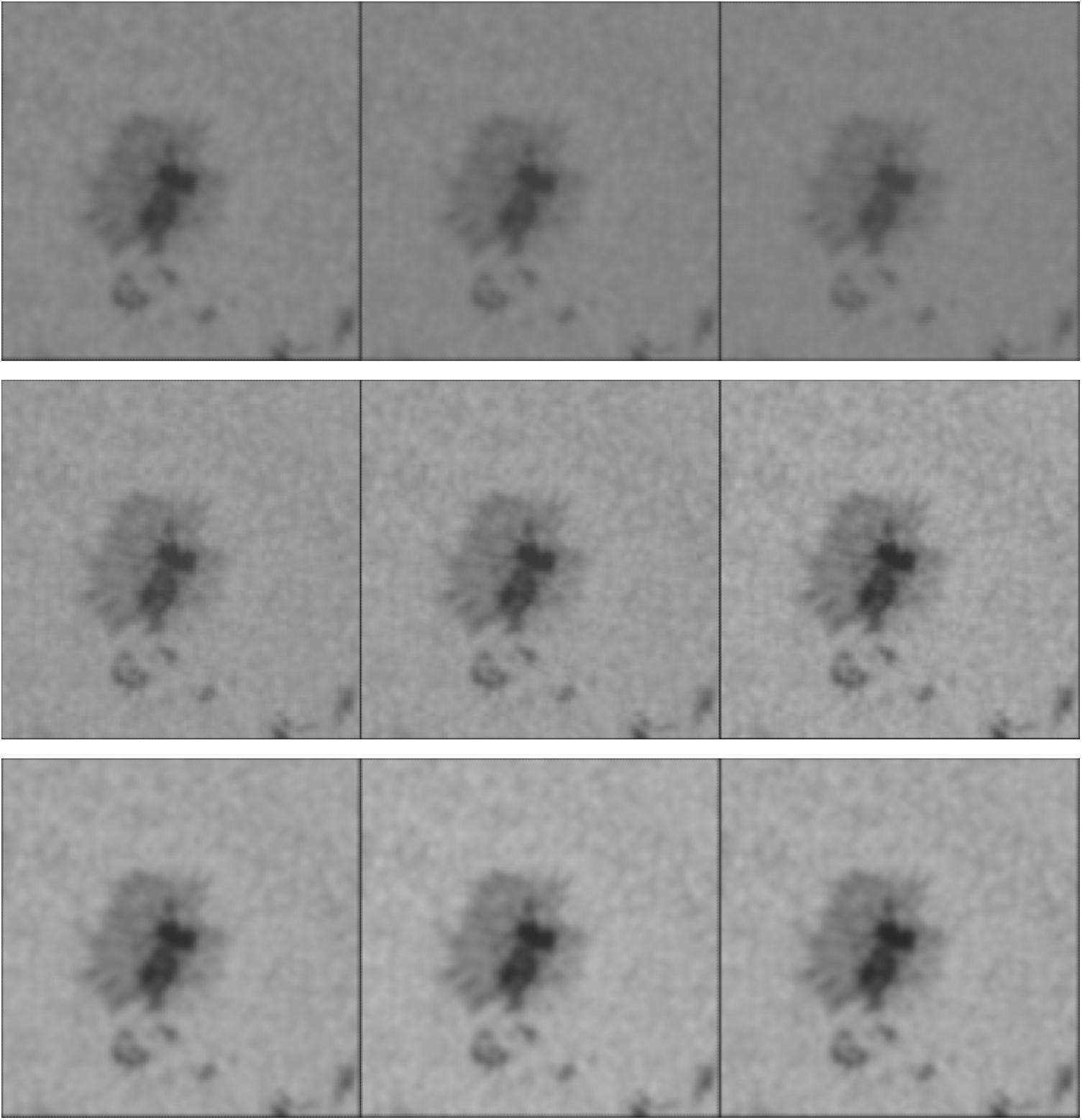
Figure 5: Visual contrast with training deepening (upper: TA network with SIFT, middle: TA network with generated GST, lower: SRCNN with HMI and GST)

Experiment 2: TA Network with generated transition images. Control the two sub-networks with the same epoch. The training data is 50 groups of pictures, each group of the pictures includes a 114×114 fuzzy HMI image, a 114×114 transition image generated by the transition network, a 456×456 clear GST image.

Experiment 3: Direct SRCNN end-to-end network from HMI images to GST images. The training data is 50 groups of pictures. Each group of the pictures includes a 114×114 fuzzy HMI image and a clear 456×456 GST image as the model input and target.

5.1 The Analysis of Traditional Evaluation Criteria

PSNR and SSIM are common evaluation criteria for image quality. PSNR calculates the mean square deviation between the source images and the target images as the denominator, the maximum value of the pixels is the numerator, the final value is given by taking the logarithm of the fraction and multiplying it by a fixed multiple. SSIM constructs brightness, contrast, and structure functions with image grayscale, standard deviation, and variance respectively. The overall similarity is the product of three functions.

PSNR and SSIM are the most widely used image evaluation indicators. The former compares the pixel value difference between the two images to evaluate image quality, while the latter uses three statistical indicators of pixel value distribution to evaluate image quality in three aspects. And they directly consider pixel value without the clarity of the reconstructed images or the macro-similarity of the feature.

Figure 6: Comparison between PSNR and SSIM with the training

Fig. 6 describe the changes of PSNR and SSIM of the TA Network and SRCNN with the deepening of training. We find that the PSNR and SSIM of the traditional SRCNN network increase slowly, while those of the TA Network decrease step by step with the deepening of training. However, with the visual effect of Fig. 5, we find that the visual effect of the SRCNN network is getting worse and worse during the process, and the features gradually become fuzzy, and the background color is gradually deepened, which is close to the background style of the GST image. We found that the PSNR and SSIM of SRCNN network are improved by constantly learning the average gray level of the GST image background, but the image details are gradually lost. In the training process of the two TA Networks, while the image style transformation, the recovery of details is strengthened, and the feature clarity is better.

5.2 Matching Rate Based on Feature Matching

Since the traditional evaluation criteria are not suitable for the application of cross-type images, a new evaluation criterion named matching rate is proposed, which is mainly based on the feature matching mechanism. The new evaluation criterion needs to measure the image clarity as well as the feature distortion. We use feature points with strong anti-interference capability to measure the two abilities. The number of feature points to reflect the clarity of the reconstructed, and the matching degree between the generated image feature points and GST image feature points is used to reflect the feature distortion. Feature points widely exist in the corner of the object boundary, which is the highest density of image information area. The number of feature points can indicate the amount of information in image reconstruction. If the feature points with high information and anti-interference can’t match the target image, it indicates that the reconstruction information is distorted and the reconstruction quality is still unsatisfactory.

The matching proportion and the reconstruction amount of feature points are respectively called similarity and clarity, and the product is used as the final evaluation criterion matching rate. When calculating the similarity, the overlapped parts of the two images are recorded as S1 and S2 respectively. Then the feature point extraction function E() is used to calculate E(S1) and E (S2) respectively to obtain the feature point matrix. The similarity is defined as follows:

R1=∑ M(E(S1),E(S2))min(∑ E(S1),∑ E(S2))(3)

where the numerator part is the matched pairs amount of feature points, and the denominator part is the maximum possible matched pairs, and the similarity range is 0 to 1. When calculating the clarity, the overlapping parts S1 and S2 of two images are also used to calculate E(S1) and E(S2). The definition of clarity is as follows:

R2=∑ E(S1)∑ E(S1)+∑ E(S2)(4)

The final matching rate is as follows:

R=R1×R2=(∑ M(E(S1),E(S2)))×∑ E(S1)min(∑ E(S1),∑ E(S2))×(∑ E(S1)+∑ E(S2))(5)

The feature point extraction function E(X) and the feature point matching function M(X, Y) can be adjusted according to the application. In the super-resolution reconstruction from HMI to GST, the overlapped part is the whole processing image. We use the SIFT to extract the feature points and use RANSAC and KNN as the feature point matching function M(X, Y). Although the feature points are obtained by SIFT, they are not specially processed and do not affect the feature matching process.

With the clarify, similarity at Fig. 7 and the matching rate at Fig. 8, it can be found that the traditional SRCNN’s ability to recover features continues to decline, and the combination of clarity and similarity indexes further verified our previous guess. In cross-type images, direct training of the end-to-end network is prone to feature blurring and background conversion, which can improve PSNR and other criteria but greatly lose image clarity. In the transition-amplification network, adding the transition images and splitting the network can improve the matching degree, reduce the difficulty of training, and greatly improve the image reconstruction quality.

Figure 7: Changes of clarify, similarity with the training

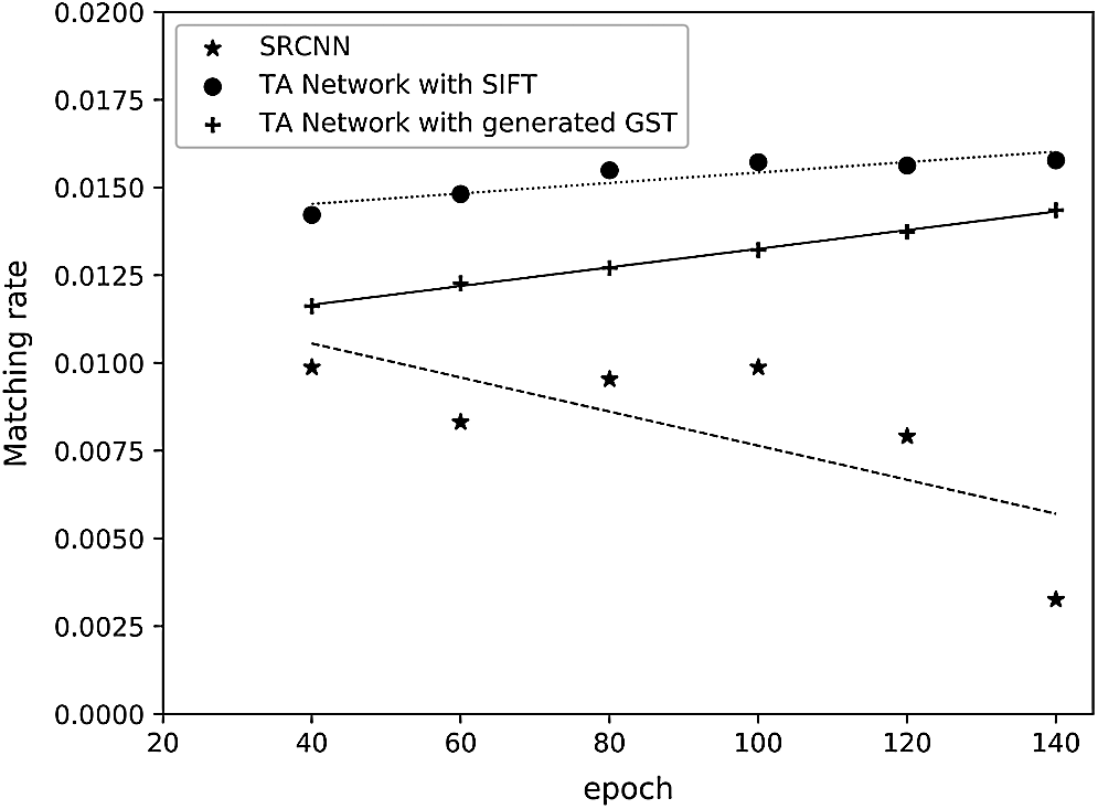
Figure 8: Changes of matching rate with the training

6  About Transfer-Learning

The above experiments (Tab. 1) have proved that the TA Network has a good effect on reducing the feature difference and offset between the source images and the target images. An intuitive idea is to discard HMI images in training and directly use GST images and their down-sampled images, which belongs to transfer-learning problem. We combine the pix2pix algorithm with a strong image conversion ability to do further experimental analysis.

Table 1: SRCNN experimental results (Net1:SRCNN, Net2:TA network with SIFT, Net3; TA network with generated GST)

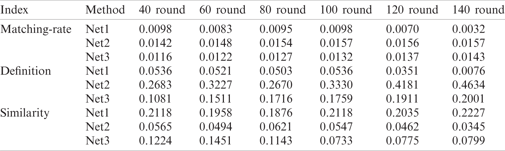
Figure 9: Different dataset comparison, upper from left to right (PIX2PIX with HMI and GST, TA network with generated transition images, original HMI image), down from left to right (PIX2PIX with down-sampling GST and GST, TA network with down-sampling GST and generated transition images, original GST image)

The experiment includes four networks: super-resolution network with HMI and GST, TA Network with HMI and GST, super-resolution network with GST and its down-sampling, TA Network with generated GST and GST. The data set and other environment is the same as the above. Due to using GST down-sampling images, the source images are naturally aligned with the target images, we do not need transition images produced by SIFT and homography matrixes.

The experimental results are shown in Fig. 9. For the two kinds of networks using HMI images as the input, the TA Network has better reconstruction quality for highlight part of umbra, but both have poor recovery effects on the fiber part of penumbra (radial texture) and typical lightspot (rice grain texture). The two networks using down-sampling GST images as input have better reconstruction quality. Networks using down-sampling GST produces some wavy distortion texture, which may be generated by individual high-weight convolution kernel. Transition-amplification network has better reconstruction quality for umbra fiber, and the reconstruction on lightspot is also clearer.

When GST down-sampling is used as the source images, the reconstruction performance of the basic GST down-sampling-GST network is much higher than that of the transition amplification network using HMI image as the source images. For large-scale umbra (block black part), the influence of source image change on reconstruction quality is not obvious, while that of smaller scale penumbra fiber and typical lightspot is huge. The reception field of a deep-learning network is directly controlled by the size of the convolution kernel. Small features are more easily affected by feature offset. When the offset distance approaches or exceeds the convolution kernel radius, the network will lose the ability to learn such small features. When using down-sampling GST as input, there is no feature offset between the source images and the target images, and the reconstruction will be better.

When facing cross-type applications, transfer-learning is worth considering. Whether it is directly using the high matched data to train the network or inheriting its weights to train further, it has a positive effect on improving the reconstruction quality.

7  Conclusion

We propose the Amplification Network for HMI images and confirm that the matching degree between the source images and target images has a great impact on network performance. We also optimize data feature offset to avoid reconstruction ability decreasing. Feature alignment can be better by adding a transition image. Both cross-type network or network using transfer-learning will be worked. The process of TA Network includes the generation of transition images, the construction of the transition network, and the construction of the amplification network.

Acknowledgement: The algorithm implementation and writing were mainly completed by Xiangchun Liu, Zhan Chen. Wei Song provided the methodology, experimental environment and the treasured suggestions on writing. Fenglei Li, and Yanxing Yang participated in the implementation of the algorithm.

Funding Statement: This work was supported in part by CAS Key Laboratory of Solar Activity, National Astronomical Observatories Commission for Collaborating Research Program (CRP) (No: KLSA202114), National Science Foundation Project of P. R. China under Grant No. 61701554 and the cross-discipline research project of Minzu University of China (2020MDJC08), State Language Commission Key Project (ZDl135-39), Promotion plan for young teachers’ scientific research ability of Minzu University of China, MUC 111 Project, First class courses (Digital Image Processing KC2066).

Conflicts of Interest: The authors declare that they have no conflicts of interest to report regarding the present study.

This work is licensed under a Creative Commons Attribution 4.0 International License, which permits unrestricted use, distribution, and reproduction in any medium, provided the original work is properly cited.