Computers, Materials & Continua DOI:10.32604/cmc.2021.017275
Article

Gait Recognition via Cross Walking Condition Constraint

Runsheng Wang1, Hefei Ling*,1, Ping Li1, Yuxuan Shi1, Lei Wu1 and Jialie Shen2

1HuaZhong University of Science and Technology, Wuhan, 430074, China
2Queen’s University, Belfast, BT7 1NN, UK
*Corresponding Author: Hefei Ling. Email: lhefei@hust.edu.cn
Received: 23 January 2021; Accepted: 25 February 2021

Abstract: Gait recognition is a biometric technique that captures human walking pattern using gait silhouettes as input and can be used for long-term recognition. Recently proposed video-based methods achieve high performance. However, gait covariates or walking conditions, i.e., bag carrying and clothing, make the recognition of intra-class gait samples hard. Advanced methods simply use triplet loss for metric learning, which does not take the gait covariates into account. For alleviating the adverse influence of gait covariates, we propose cross walking condition constraint to explicitly consider the gait covariates. Specifically, this approach designs center-based and pair-wise loss functions to decrease discrepancy of intra-class gait samples under different walking conditions and enlarge the distance of inter-class gait samples under the same walking condition. Besides, we also propose a video-based strong baseline model of high performance by applying simple yet effective tricks, which have been validated in other individual recognition fields. With the proposed baseline model and loss functions, our method achieves the state-of-the-art performance.

Keywords: Gait recognition; metric learning; cross walking condition constraint; gait covariates

1  Introduction

Gait, as a type of effective biometric feature, can be used to identify persons at a distance. Since gait is an unconscious behavior, it can be recognized without cooperation of subjects. Therefore, besides person re-identification approaches [1,2], gait recognition methods have extensive deployment prospect on surveillance video and public security. Recent years, gait recognition has attracted the attention of many researchers. The past years has witnessed the rapid development of deep learning in image recognition and retrieval [3–5]. With the development of deep learning, many neural-network-based gait recognition methods are proposed. Typically, gait recognition can be divided into image-based methods and video-based methods.

Image-based methods [6–8] take Gait Energy Images (GEI) as input and use CNN to judge whether the input GEI pair belongs to the same identity. Reference [9] introduces GAN to get rid of the adverse influence of viewpoints. However, GEI-based methods which take image as input cannot capture spatial temporal gait information. Video-based methods capture motion pattern from a gait sequence. Reference [10] uses LSTM to extract feature from pose estimated by OpenPose to get rid of the adverse influence bag-carrying and clothing. Recently proposed video-based methods focus on aggregating frame-level features from silhouettes sequence via temporal pooling such as GaitSet [11] and GaitPart [12], and use triplet loss as supervision signal. These methods achieve the state-of-the-art performance.

Nevertheless, one issue of gait recognition is that the variance of walking conditions or gait covariates, i.e., normal walking (NM), bag carrying (BG) and clothing (CL), changes the appearance of gait silhouettes. As shown in Fig. 1, the visual differences of cross walking condition intra-class GEI pairs ((a) and (b), (a) and (c)) are large, while the visual difference of inter-class GEI pair from the same walking condition ((a) and (d)) is small.

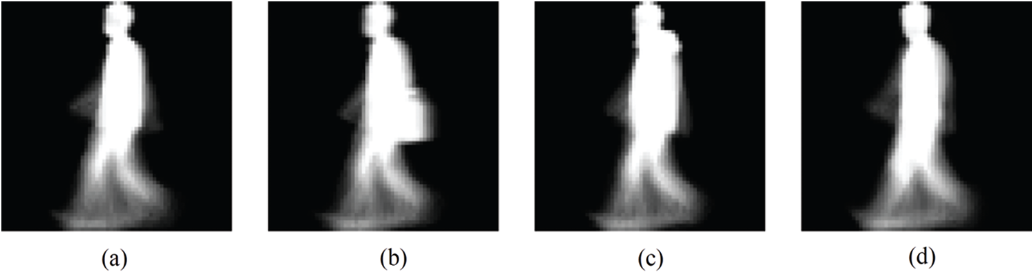
Figure 1: Gait covariates change the appearance of GEI (synthesized by a sequence of silhouettes). (a) is the GEI of NM. (b) and (c) are GEI of BG and CL, respectively. (a)–(c) belong to the same identity. (d) is the GEI of NM from another identity

Thus, the issue of variance of walking conditions results in large distance of positive pairs from different walking conditions, as well as small distance of negative pairs from the same walking condition. Unfortunately, this issue is ignored by the state-of-the-art video-based methods which only employs triplet loss [13] and do not explicitly take walking conditions into account and results in the large intra-class distance and small inter-class distance. We attach more importance on the cross-walking-condition samples, and aim at devise loss functions to explicitly reduce the distance of intra-class gait samples under different walking conditions and enlarge the distance of inter-class gait samples under the same walking condition at feature space. This approach is referred as cross walking condition constraint. Practically, we design center-based and pair-based loss functions.

The center-based loss is named as cross walking condition center loss (XCenter loss). Specifically, this loss contracts the intra-class centers of different walking conditions as well as repulses the inter-class centers of same walking condition. The pair-based loss named as cross walking condition pair-wise loss (XPair loss), which focuses on local pair-wise similarity, intends to decrease distance of cross walking condition positive pairs, as well as enlarge the distance of same walking condition negative pairs.

Secondly, we propose a strong baseline model of high performance for video-based gait recognition by applying simple yet effective tricks, which have been validated in other individual recognition fields [14]. Specifically, we involve batch normalization (BN) layers in our model to mitigate the covariate shift issue as well as make the model easier to train, and combine identification loss (ID loss) and metric learning as the training signal. We also use the second-order pooling for frame-level part feature extraction. With these simple tricks, our baseline model achieves high performance.

Our contributions can be summarized as follows:

•   We propose cross walking condition embedding constraint to explicitly constrain distance between gait samples under different walking conditions, and enlarge the distance of inter-class samples under the same walking condition.

•   We explore tricks which is beneficial for the training of the model. With these tricks, we devise a stronger video-based gait recognition baseline model of high performance. The baseline model can be further used in the future researches.

•   Compared with other existing methods, we achieve a new state-of-the-art performance of cross-view gait recognition on CAISA-B and OU-MVLP dataset. We further validate the proposed methods by ablation experiment.

2  Related Work

2.1 Video-Based Gait Recognition

Video-based methods take a sequence of gait silhouettes as input and aggregate frame-level features into a video-level feature. Reference [15] uses LSTM and CNN to extract spatial and temporal gait features. Reference [16] apply 3D convolution operation on feature maps of frames. GaitNet [17] disentangles gait features from colored images via novel losses and uses LSTM to extract temporal gait information. Recently, GaitSet and GaitPart, as video-based methods, focus on aggregating features from gait silhouettes via spatial pooling and temporal pooling. GaitSet [11] extract frame-level feature by CNN and then propose Set Pooling (SP), which is practically an order-less temporal max pooling, to generate the video-level feature map. GaitPart [12] capture temporal information by a short-term motion capture module. These video methods focus on capturing discriminative spatial temporal information, yet do not explicitly consider the issue of gait covariates. Our method is closely related with GaitSet [11] and GaitPart [12], both of which achieve the state-of-the-art performance, and focuses more on cross walking condition gait recognition.

2.2 GEI-Based Cross Walking Condition Gait Recognition

In the real situation, gait representation can be interfered by bag-carrying or clothing change (referred as variance of walking condition), since the real shape of human and motion pattern of limbs are invisible or occluded by clothes. Many GEI-based methods strive for cross walking condition gait recognition. Early works [6,18] design networks to learn the similarity of cross walking condition GEI pairs. Reference [7] learn the similarities of GEI pairs in a metric learning manner. Some works devise Generative Adversarial Network (GAN) based methods to solve this issue. Generative methods [9,19] use GAN based methods to overcome the influence of variance of views. References [9,20] generate GEI images of normal walking condition. Reference [21] uses AutoEncoder based network disentangles gait features from GEI of different walking condition to get rid of the influence of clothing and bag-carrying. Reference [22] designs a visual attention-based network to focus on limbs that is invariant for clothing change. However, these GEI-based methods fail to capture dynamic motion information, since they only take one image as input, and cannot take advantages of the recently proposed video-based model, which achieve the state-of-the-art performance.

3  Proposed Method

In this section, we first introduce the loss functions, designed for cross walking condition constraint, i.e., XCenter and XPair loss, in Sections 3.1 and 3.2. Then, we introduce the framework of the proposed baseline model, and simple yet effective tricks involved in the framework.

3.1 Cross Walking Condition Center Loss (XCenter)

In this section, we present our cross-walking-condition center loss, which is named as XCenter loss. As discussed in Section 1, the variance of walking conditions results in large intra-class discrepancy and small inter-class discrepancy. Two manipulations of centers are proposed. The first manipulation is the Center Contraction Loss (CCL) which intends to decrease the distance of intra-class centers to reduce the discrepancy of intra-class distribution, while the second manipulation is Center Repulsion Loss (CRL) which manages to repulse the inter-class centers of the same walking condition to enlarge the inter-class distance.

Computation of Centers: We compute the centers of samples under different walking condition for each identity. Take i-th identity we sample in a mini-batch, the centers of three walking conditions, i.e., normal walking (NM), bag-carrying (BG) and clothing (CL) are computed as:

cinm=1|Snmi|∑j∈Snmifj,cibg=1|Sbgi|∑j∈Sbgifj,cicl=1|Scli|∑j∈Sclifj(1)

Here, Snmi, Sbgi and Scli are three sets of samples of i -th identity of NM, BG and CL, respectively. cinm, cibg, cicl denote three centers of i -th identity of the three walking conditions, which are computed by averaging the features of corresponding walking conditions (denoted as fj in the above equation). Note that the computation of centers is conducted within a mini-batch.

Center Contraction Loss (CCL): To reduce the intra-class discrepancy, we propose a loss named as Center Contraction Loss (CCL) that helps the intra-class centers contract. Since the gait samples of NM are not interfered by other gait covariates (clothing and bag-carrying) and represent the real gait information of humans. As shown in Fig. 2a, we intend to decrease the distance between the center of NM and the intra-class centers of other two walking conditions.

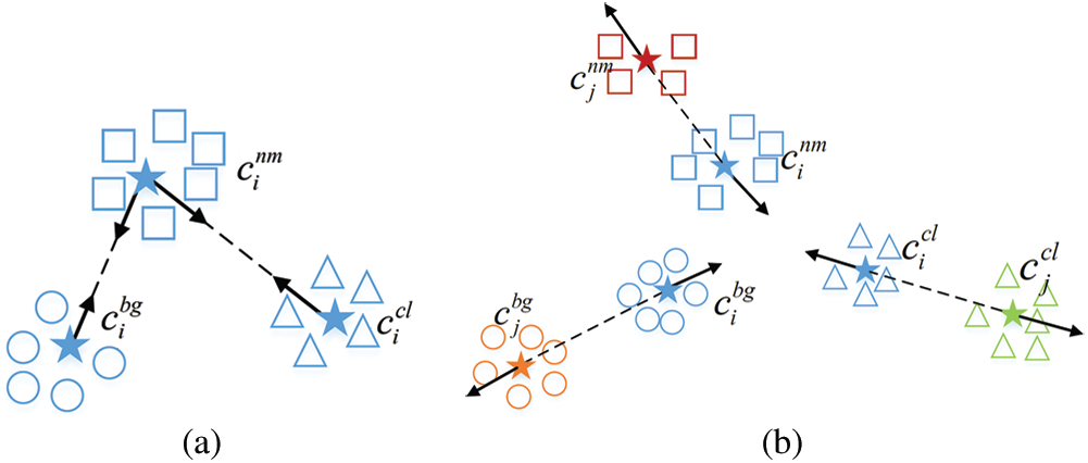
Figure 2: A diagram of XCenter loss. (a) Center contraction loss (CCL), (b) Center repulsion loss (CRL)

Points of different color represent samples of different identities. Squares, circles, and triangles denote samples of NM, BG and CL, respectively. The solid stars enclosed by samples denote the centers of corresponding samples. Fig. 2a is the diagram of CCL, where intra-class centers of different walking conditions (stars of same color yet enclosed by points of different shape) are pulled closer. Fig. 2b is the diagram of CRL, where the inter-class centers of the same walking condition (stars of different colors yet enclosed by points of same shape) are repulsed. Thus, CCL can be represented as:

Lcon=1K∑i=1Kd(cinm,cibg)+d(cinm,cicl)(2)

where K is the number of identities in a mini-batch, and d(⋅,⋅) measures the Euclidean distance of two given centers. d(cinm,cibg), d(cinm,cicl) denote the Euclidean distance between the center of NM and the center of BG, the center of NM and the center of CL, respectively.

Center Repulsion Loss (CRL): We design a center-based repulsion loss to enlarge the discrepancy of interclass samples under the same walking condition. As shown in Fig. 2b, CRL repulses the inter-class centers under the same walking condition away. CRL can be expressed as follow:

Lrep=1K∑i,t[m-minj≠id(cit,cjt)]+(3)

Here, subscript i and superscript t are the indicator of identities and walking conditions (i∈{1,2,…,K} and t∈{nm,bg,cl}), respectively. j is the indicator of negative identities. [⋅]+ denotes the hinge function. This loss enlarges the distance of the hardest inter-class centers of the same walking condition. The XCenter loss can be represented as:

Lxcen=Lcon+Lrep(4)

3.2 Cross Walking Condition Pair-Wise (XPair) Loss

As shown in Fig. 3, we also design a pair-wise loss function which focuses on local sample pairs. Intuitively, the dissimilarity of cross walking condition positive (Xpos) pairs should be decreased, while the distance of same walking condition negative (Sneg) pairs should be enlarged. Thus, XPair loss consists of two loss functions.

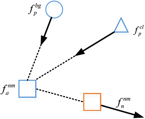
Figure 3: The diagram of XPair loss

We reduce the distance of sample pairs from the same identity (same color) yet different walking condition (different shape), and enlarge the distance of pair from different identities (different color) yet same walking condition (same shape).

Xpos Pair Loss: This loss intends to decrease the dissimilarity of cross walking condition positive (Xpos) pairs. Similar with Section 3.1, we intend to minimize the distance between samples of NM and samples of other two walking condition. Two corresponding sorts of cross walking condition pairs are selected.

LXpos=1|Snm|∑a∈Snm|Snm|maxpd(fanm,fpbg)+maxpd(fanm,fpcl)(5)

Here, fanm is the anchor feature of NM. fpbg and fpcl are the positive features of BG and CL, respectively. This loss decreases the dissimilarity of two kinds of cross walking condition hardest sample pairs.

Sneg Pair Loss: This loss intends to enlarge the distance of negative yet of same walking status (Sneg) pairs. Practically, hardest negative pairs of NM, which is of smallest dissimilarity, are selected:

LSneg=1|Snm|∑a∈Snm|Snm|[m-minnd(fanm,fnnm)]+(6)

Here, n is the indicator of negative samples of anchor a . fnnm is the negative feature of NM. m is the margin for Sneg pair. The XPair consists of the above two loss functions, and can be represented as:

Lxpair=LXpos+LSneg(7)

3.3 Framework with Effective Tricks

Typical video-base gait recognition framework includes frame-level feature extractor, aggregation of video-level feature, horizontal mapping and part-level feature learning. The framework of our model, as shown in Fig. 4, also consists of the above components. The framework takes a sequence of gait images, the length of which is T , as input. In the following, we introduce the details and proposed tricks of all the components.

The frame-level feature extractor generates a matrix of temporal part features, Z=(zp,i)P×T, which represents features of P parts and T frames. SP represents Set Pooling. BNHM denotes Horizontal Mapping with BN layers. SP and BNHM are applied on each part to generate the final video-level part features f1,f2…fP. Then ID loss with BNNeck, triplet loss and proposed loss functions are used for supervision.

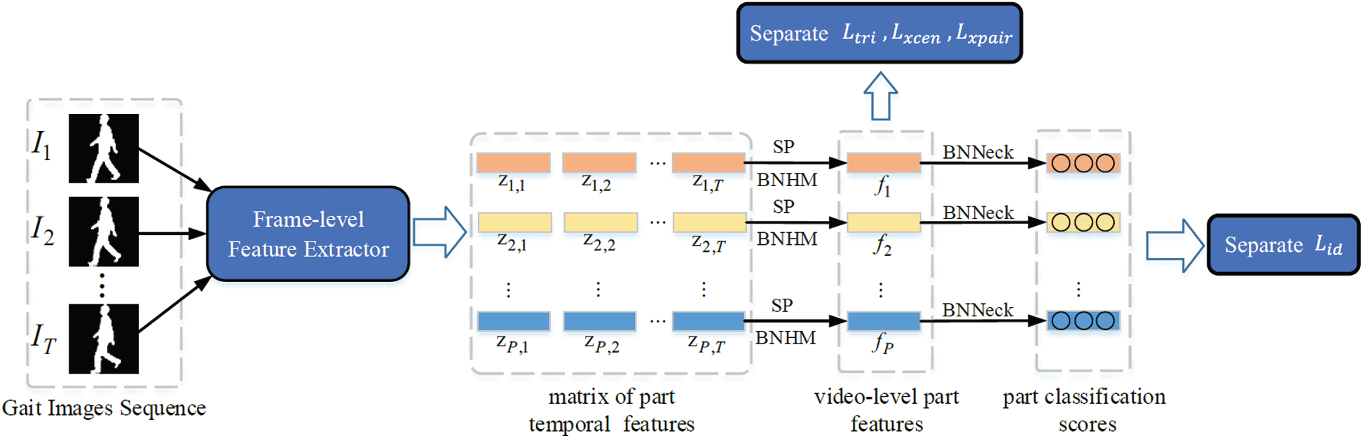
Figure 4: The overall framework of our method

Frame-Level Feature Extractor with PSP: As shown in Fig. 5, a base CNN network is used to extract feature maps for frames. For i-th frame, the extraction of the base network is as:

Xi=F(Ii)(8)

Here, Ii denotes i-th gait image. and Xi is the feature map of Ii. F represents the base convolution neural network. Then, Xi is partitioned into horizontal part-level feature maps.

Xi=(X1,i,X2,i,…,XP,i)(9)

We also use second-order pooling to generate features for different parts, which is called as Part-based Second-order Pooling (PSP) and is introduced in Section 3.4.

zp,i=PSPp(Xp,i)(10)

Here, P is the number of parts and p∈{1,2,…,P}. zp, i represents the feature of p-th part of i-th frame. As shown in Fig. 5, parallel PSP blocks produce features for horizontal parts.

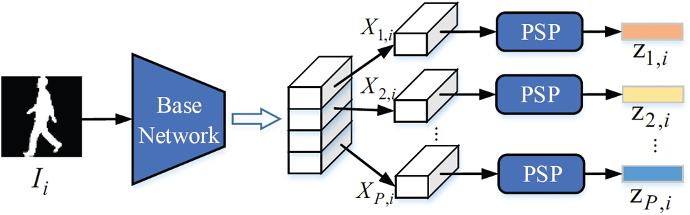
Figure 5: Frame-level feature extractor

Aggregation of Video-Level Feature: As shown in Fig. 4, given T frames, PSP blocks produce the matrix of part temporal features Z=(zp,i)P×T, which represents features of P parts and T frames. Previous work [12] also produce similar feature matrix. Temporal features of each part are aggregated into video-level part feature by Set Pooling (SP) [11]. Taking p-th part as an example, the p-th part video-level feature mp generated by SP can be expressed as:

mp=SP(zp,1,zp,2,…,zp,T)(11)

Usage of BN (BNHM and BNNeck): Since the gait dataset has many different types of gait samples, it is hard to sample all types of data in a mini-batch. This causes the issue of covariate shift. Thus, we involve BN layers in our framework. First, horizontal mapping uses part independent FC layers to project part video-level features into discriminative space. We combine horizontal mapping with BN layers, which is named as BNHM. The p-th part BNHM which generates p-th part video-level feature fp can be denoted as fp=FC(BN(mp)). Secondly, we also involve identification loss (ID loss) in the training process with BNNeck [14]. Practically, the part feature fp first goes through a BN layer, fpbn=BN(fp). And ID loss takes fpbn as input.

Part-Level Feature Learning: For the baseline model, only ID Loss and triplet loss are involved. For our model, as shown in Fig. 4, ID Loss, Triplet loss, and proposed XCenter, XPair loss are applied separately on each part, where ID loss is applied with BNNeck while other loss functions are applied directly on video-level part features.

3.4 Part-Based Second-Order Pooling (PSP)

We use part-based second-order pooling to extract discriminative frame-level part features, since the second-order pooling increases the non-linearity for features and is able to capture discriminative high-order information [23,24].

Suppose that frame-level part feature map Xp, i given in (10) is of c×hw dimensions (denote channel, height, and width, as shown in Fig. 6). For simplicity, subscripts p, i are ignored below. Typically, second-order pooling of X (denoted as B(X)) generate image representation by computing channel-wise covariance matrix:

B(X)=vec(XXT)(12)

Here, vec represents vectorization, and B(X)∈ℝc2, which is of high dimensions. Recent years, many works [25,26] focuses on reducing the computational cost and memory requirement for second-order pooling. We also formulate a light weight second-order pooling module.

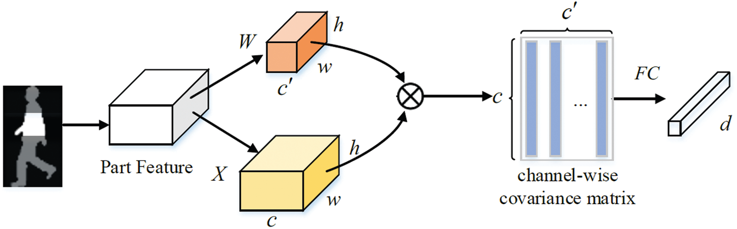
Figure 6: Structure of part-based second-order pooling (PSP)

As shown in Fig. 6, we replace XT with WT in (12). Thus, B(X)=vec(XWT), where W is another part-level feature map generated by a convolutional layer, and the dimension of W is c′×HW, where c′<c. The dimension of B(X) is reduced and B(X)∈ℝcc′. To further reduce the dimension of the matrix, a FC layer is followed to generate the final frame-level part feature of d dimension. Thus, PSP that generates frame-level part feature z can be expressed as:

z=B(X)=FC(vec(XWT))(13)

Note that the PSP blocks are applied on horizontal parts and the parameters of FC layers of PSP are part independent.

3.5 Overall Loss Function

In this part, we first introduce the base loss function which consists of triplet loss and identification loss. Then the overall loss is presented. Base Loss Identification loss and triplet loss are involved in the training process, which are separately applied on each part. The triplet hard loss can be represented as:

Ltri=∑a=1M[maxp∈ℙ(a)d(fa,fp)+m-minn∈ℕ(a)d(fa,fn)]+(14)

where a, p and n represent anchor, corresponding positive and negative sample, respectively. ℙ(a) and ℕ(a) represent the sets of positive samples and negative samples of the given anchor. Different from previous work [11,12], we also incorporate identification loss during training. The features go through a BN layer and FC layer (BNNeck [14]) to generate the classification scores. Thus, the identification loss can be denoted as:

Lid=-∑k=1M log(eWykTfkbn∑c=1NeWcTfkbn)(15)

Here, superscript bn denotes the features generated by the BN layer, and subscript ⋅k denotes k -th sample in the mini-batch. N is the number of identities in the training set. Wc denotes the weight vector of c -th class, and Wyk is the weight vector of the ground truth identity of k -th sample. The combination of Ltri and Lid are referred as base loss functions: Lb = Ltri + Lid.

Overall Loss: The overall loss includes hard triplet loss, identification loss, XCenter loss and XPair loss. The equation of overall loss function can be expressed as:

L=Lb+λxcenLxcen+λxpairLxpair(16)

where λxcen and λxpair control the importance of XCenter loss and XPair loss, respectively.

3.6 Implementation Details

Experiments are implemented based on pytorch with an Nvidia RTX2080Ti GPU. In this part, we introduce the configuration and details of our network. The input silhouettes, the channel of which is set as 1, are cropped into 64×44 in all experiments. For fair comparison, we adopt the same backbone used in previous video-based model [11]. The output channels of each layer in backbone are 32, 32, 64, 64, 128, 128. As for the PSP used in frame-level feature extractor, W mentioned in Section 3.4 is generated by an extra convolutional layer. The channel of W (defined as c′ in Section 3.4) is set as 32. The dimension of frame-level part feature, i.e., d defined in Section 3.4, is set as 256. The Set Pooling is set as max pooling, since previous works [11,12] validate that this setting achieves better performance. The dimension of the final video-level part feature fp is set as 256.

4  Experiment

Two prevailing gait recognition benchmarks, CASIA-B and OU-MVLP, are included in our experiments. In this section, we first introduce two datasets, and then comparative and ablative results are given. In comparison experiments, we report the state-of-the-art models and proposed method on the two datasets. We also visualize the gait features to validate whether the proposed loss functions decrease the intra-class discrepancy.

4.1 Datasets

CASIA-B [27] dataset contains 124 identities. Although the number of subjects is limited, each subject has 110 samples of 11 different views and 10 walking types, and the 10 walking types consists of 6 types of normal walking condition (indexed as nm-01—nm-06), 2 types of bag carrying (BG) (indexed as bg-01, bg-02) and 2 types of clothing (CL) (indexed as cl-01—cl-02). Thus, the dataset contains samples for cross-view and cross-condition evaluation. During training, the samples of first 74 subjects are taken as training data. During testing, the samples of the rest subjects are involved. Concretely, the samples from nm-01–nm-04 are taken as probes. The samples of other types are taken as gallery.

OU-MVLP [28] is a gait dataset of largest population in the world. It contains 10307 persons. 5153 persons consist training set and the other 5154 persons consist testing set. Each person has image sequences of 14 views. The views consist of two groups: (0∘,15∘,…,90∘) and (180∘,195∘,…,270∘), and each view of one person have two gait sequences, where the sequences indexed 01 are used as probes and the sequences indexed 02 are used as gallery, during training.

Evaluation Protocol: For fair comparison, we use cross-view evaluation protocol which is employed in previous work to measure the performance of our model. During evaluation, the probes are used to retrieve the gallery of different views, and mean rank-1 accuracy of galleries of other views is reported. Except for cross-view evaluation, cross-walking-condition evaluations are considered in CASIA-B, which use probes to retrieve the galleries of different walking conditions in the cross-view manner.

Training Parameters: During training, Adam Optimizer is employed in all experiment, where the momentum is 0.9 and the learning rate is 1e −4. The margin of triplet loss is set as 0.2. The margin of CRL is set as 0.5. Batch size can be denoted as (p, k), where p represents the number of subjects, and k represents the number of samples selected from each subject. The batch size of experiment implemented on CASIA-B is (4, 16). We train our model for 15K iterations, which is notable that our model converges significantly faster than previous state-of-the-art models [11,12] during training. In the experiment of OU-MVLP, the batch size is set as (32, 4). We train our model on OU-MVLP for 150K iterations. The learning rate decays to 1e −5 in the last 50K iteration. Since OU-MVLP only contains gait sequences of normal walking condition, proposed loss functions ( Lxcen and Lxpair) is not involved in the experiment.

4.2 Comparison Experiment

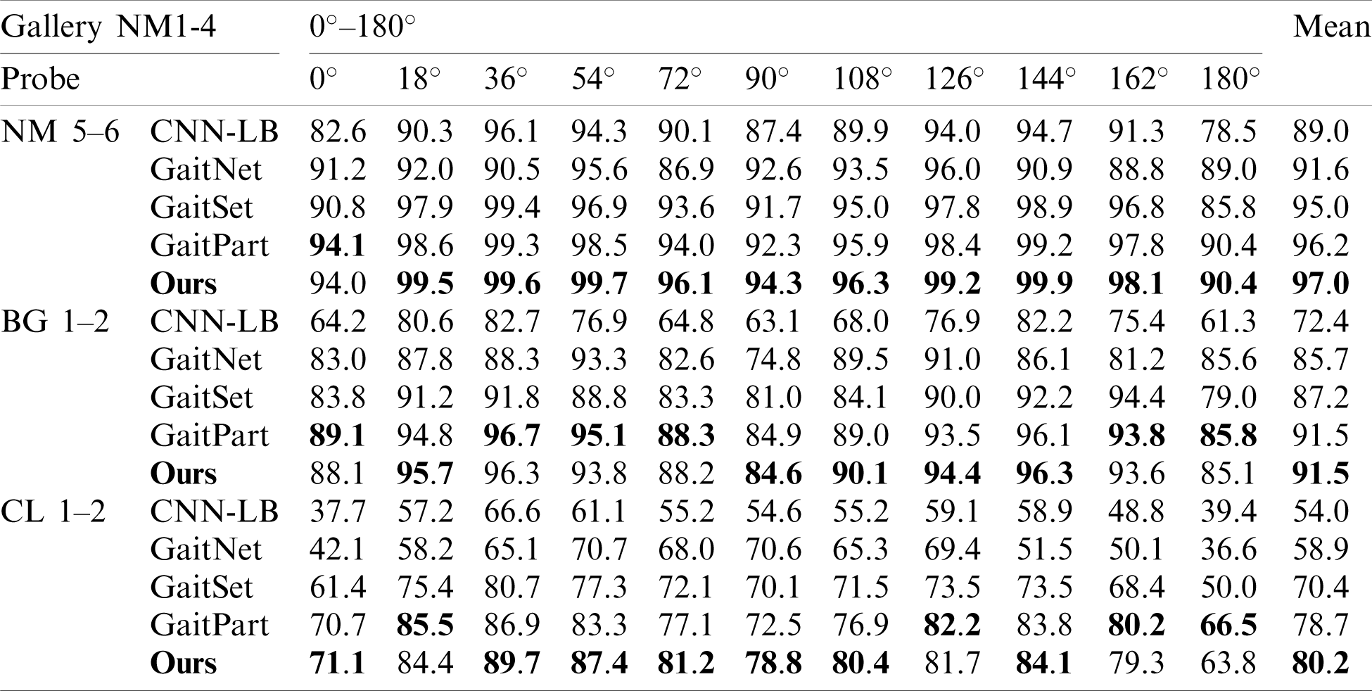
Comparative results on CASIA-B and OU-MVLP are given in Tabs. 1 and 2, respectively.

CASIA-B: Tab. 1 demonstrates the cross-view and cross walking condition recognition result. As shown in the table, our method achieves the state-of-the-art result. For the three walking conditions, we report the rank-1 accuracy of different probe view and the average rank-1 accuracy for different walking condition. Our model achieves 97% and 80.2% rank-1 accuracy under NM and CL. This performance surpasses most of cross-view gait recognition methods to our best knowledge. Several conclusions can be observed: 1) Compared with CNN-LB which takes GEI as input, our method and other video-based methods perform better. This further demonstrates the superiority of video-based methods [11,12] which aggregate frame-level features via temporal pooling or set pooling. 2) Compared with GaitNet [17], our method achieves better results. Both of our method and GaitNet intend to mitigate the adverse impact of the variance of walking conditions on the extraction of gait features. GaitNet introduces LSTM and auto-encoder based disentanglement learning to extract walking condition invariant gait features, while our method intends to apply simple yet effective loss functions to alleviate the discrepancy of the gait features from different walking conditions. 3) Our method is better than GaitSet [11] and GaitPart [12] which are so far the state-of-the-art approaches. Specifically, the two cross walking condition recognition performance (reported by the rows of BG and CL in Tab. 1) surpass [11,12] by a large margin. We believe the reason is that the proposed loss functions focus more on cross walking condition gait recognition, while GaitSet and GaitPart simply use BA+ triplet loss [13] and do not take the variance of walking conditions into account.

Table 1: Performance of advanced methods

OU-MVLP: Since this dataset is so far the largest gait dataset, we implement experiments on this dataset to further validate our method. Tab. 2 reports performance of our method and other advanced methods under the cross-view evaluation protocol. Since the proposed loss functions focus on clothing and object carrying invariant gait recognition, and this dataset does not contain corresponding samples, we only report the performance of the proposed baseline model without using the XCenter and XPair loss functions. It can be observed that our method performs better than previous methods. Time consuming is tested on this dataset. During evaluation, which is implemented with one RTX2080Ti GPU, GaitSet costs 17 min while ours costs 10 min. Note that since the hardware setting in our experiment is different with [11], the time costed by evaluations of GaitSet reported in our implementation is different with that given in [11].

4.3 Ablation Study on Involved Tricks of Framework

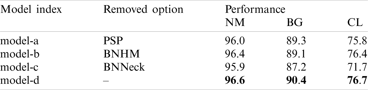
In Tab. 3, we validate several options that benefit the proposed framework, including PSP block, BNHM, and BNNeck. The results of four models are given.

Model-a replaces the PSP with max-pooling and a FC layer for fair comparison, while model-b removes the BN layers in BNHM, which is turned into ordinary horizontal mapping [11]. Model-c removes BNNeck. Model-d is the strong baseline model trained with all the proposed tricks. Both above models are trained with base loss function Lb. Following points can be observed: 1) Effectiveness of PSP: We compare model-a with model-d. It can be seen that model-d with PSP block surpasses the model-a with max pooling (first-order pooling). This indicates that the proposed light-weight second-order pooling is better for extracting local frame-level feature from gait silhouettes. 2) Effectiveness of BNHM: Model-b removes the BN layer before horizontal mapping. Obvious performance drop proves the necessity of BNHM. We believe that since the variance of walking conditions causes the discrepancy of gait features, the BN layer is beneficial for horizontal mapping. 3) Effectiveness of BNNeck: Model-c removes BNNeck and degrades in performance. This proves the effectiveness of BNNek used in our framework.

Table 2: Performance of advanced methods on OU-MVLP

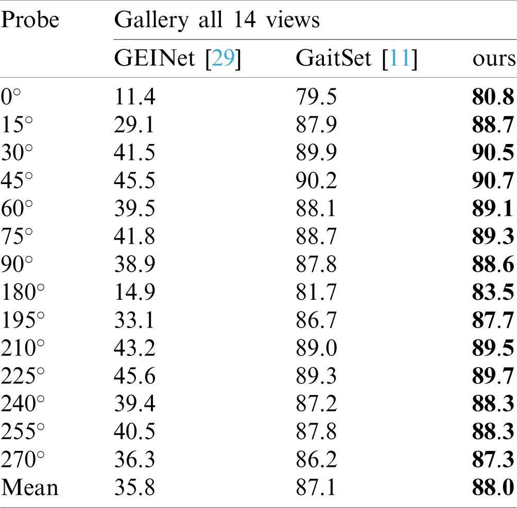
Table 3: Results of ablation study on proposed framework

The three tricks are simple and effective. Furthermore, they make the model easier to train. Our baseline model can converge after 15K iterations, while GaitSet converges after 80K iterations.

4.4 Ablation Study on Loss Functions

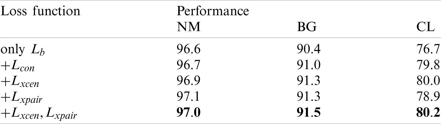
In Tab. 4, we report the ablative results of proposed loss functions. Four rows of results are given. The first row is the baseline model trained with base loss function Lb. The second row gives the result of model trained with Lb and center contraction loss Lcon. The third row gives the result of model trained with Lb function and XCenter loss Lxcen. The fourth row shows the result of model trained with Lb and XPair loss Lxpair. The last row gives the performance of the model trained with both Lb, Lxcen and Lxpair.

Columns of BG and CL in Tab. 4 report the accuracy of using NM probes to retrieve BG and CL galleries, respectively. Thus, the two columns report the performance of cross walking condition recognition. The 2-nd row is the model trained with Lb and Lcon (which means the XCenter loss without Lrep). Thus, comparison between 3-rd row and 2-nd row proves the effectiveness of Lrep. From 3-rd row and 4-th row, we can observe that both two loss functions improve the accuracy of cross walking condition gait recognition. The last row shows that joint training of two loss functions is effective for both cross view and cross walking condition recognition. Consequently, we believe the proposed loss functions are able to reduce the intra-class discrepancy caused by gait covariates. We also test λxcen and λxpair. In the experiment, λxcen is set from 0.1 to 0.5 and λxpair is set from 0.01 to 0.05. We find the best λxcen is 0.1 and the best λxpair is 0.02 for the joint training of XCenter and XPair loss.

Table 4: Ablation study on proposed loss functions

4.5 Analysis of Gait Features

The features are visualized by T-SNE [30] in Fig. 7, where Fig. 7. Fig. 7a is the visualization result of the features from the model trained with proposed losses and Fig. 7b is the result of features generated by the baseline model. It can be seen from Fig. 7b that features of CL (triangle shaped points) are separable from other features that belongs to the same person, since the triangle points can be easily circled out by the red circles. However, features from the same subject tend to stay together in Fig. 7a. It can be concluded that the intra-class divergence is decreased by the constraint of proposed methods.

We select several identities to visualize their samples, where squares, circles and triangles represent the features of NM, BG and CL, respectively. Points of different colors represent features from different identities. Fig. 7a visualizes features generated from the model trained with proposed loss functions. Fig. 7b visualizes features produced by the baseline model.

We also present the statistical result of the distance of cross walking condition positive (Xpos) pairs in Fig. 8. Blue curve is the distribution of Xpos pairs computed from the baseline model, while red curve is the distribution of Xpos pairs generated from the model trained with the constraint of proposed loss functions. It can be seen that with the constraint of Lxcen and Lxpair, the distribution shift left, which means the discrepancy of Xpos pairs decreases.

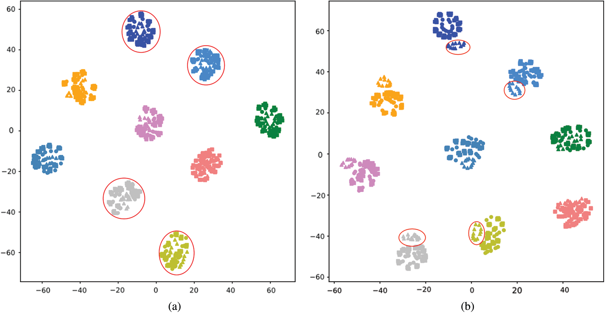
Figure 7: Visualization of features from CASIA-B by T-SNE. (a) With proposed constraint (b) baseline model

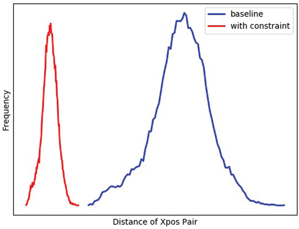
Figure 8: Distribution of distance of cross walking condition positive (Xpos) pairs

5  Conclusion

In this paper, we propose cross walking condition constraint, which specifically contains center-based and pair-wise loss, manages to constrain cross walking condition intra-class discrepancy as well as enlarge inter-class discrepancy of same walking condition. We also present a more effective video-based gait recognition model, which utilizes and simple yet effective tricks such as part-based second-order pooling, usage of BN layers and joint training with ID loss, as a strong baseline model. The proposed method achieves a new state-of-the-art performance.

Funding Statement: This work was supported in part by the Natural Science Foundation of China under Grant 61972169 and U1536203, in part by the National key research and development program of China (2016QY01W0200), in part by the Major Scientific and Technological Project of Hubei Province (2018AAA068 and 2019AAA051).

Conflicts of Interest: The authors declare that they have no conflicts of interest to report regarding the present study.

References

 1.  Y. Shi, Z. Wei, H. Ling, Z. Wang, P. Zhu et al., “Adaptive and robust partition learning for person retrieval with policy gradient,” IEEE Transactions on Multimedia, Early Access, 2020. [Google Scholar]

 2.  Y. Shi, Z. Wei, H. Ling, Z. Wang, J. Shen et al., “Person retrieval in surveillance videos via deep attribute mining and reasoning,” IEEE Transactions on Multimedia, Early Access, 2020. [Google Scholar]

 3.  H. Wu, Q. Liu and X. Liu, “A review on deep learning approaches to image classification and object segmentation,” Computers, Materials & Continua, vol. 60, no. 2, pp. 575–597, 2019. [Google Scholar]

 4.  H. Ling, Y. Fang, L. P. Li, J. Chen, F. Zou et al., “Balanced deep supervised hashing,” Computers, Materials & Continua, vol. 60, no. 1, pp. 85–100, 2019. [Google Scholar]

 5.  H. Yang, J. Yin and Y. Yang, “Robust image hashing scheme based on low-rank decomposition and path integral LBP,” IEEE Access, vol. 7, pp. 51656–51664, 2019. [Google Scholar]

 6.  Z. Wu, Y. Huang, L. Wang, X. Wang and T. Tan, “A comprehensive study on cross-view gait based human identification with deep cnns,” IEEE Transactions on Pattern Analysis and Machine Intelligence, vol. 39, no. 2, pp. 209–226, 2016. [Google Scholar]

 7.  K. Zhang, W. Luo, L. Ma, W. Liu and H. Li, “Learning joint gait representation via quintuplet loss minimization,” in Proc. of the IEEE Conf. on Computer Vision and Pattern Recognition, Long Beach, California, pp. 4700–4709, 2019. [Google Scholar]

 8.  X. Tang, X. Sun, Z. Wang, P. Yu and N. Cao, “Research on the pedestrian re-identification method based on local features and gait energy images,” Computers, Materials & Continua, vol. 64, no. 2, pp. 1185–1198, 2020. [Google Scholar]

 9.  S. Yu, H. Chen, E. B. Garcia Reyes and N. Poh, “Gaitgan: Invariant gait feature extraction using generative adversarial networks,” in Proc. of the IEEE Conf. on Computer Vision and Pattern Recognition Workshops, Honolulu, Hawaii, pp. 30–37, 2017. [Google Scholar]

10. R. Liao, C. Cao, E. B. Garcia, S. Yu and Y. Huang, “Pose-based temporal-spatial network (PTSN) for gait recognition with carrying and clothing variations,” in Chinese Conf. on Biometric Recognition, Shenzhen, China, pp. 474–483, 2017. [Google Scholar]

11. H. Chao, Y. He, J. Zhang and J. Feng, “Gaitset: Regarding gait as a set for cross-view gait recognition,” in Proceeding of the AAAI Conference on Artificial Intelligence, vol. 33, pp. 8126–8133, 2019. [Google Scholar]

12. C. Fan, Y. Peng, C. Cao, X. Liu, S. Hou et al., “Gaitpart: Temporal part-based model for gait recognition,” in Proc. of the IEEE/CVF Conf. on Computer Vision and Pattern Recognition, Virtual, pp. 14225–14233, 2020. [Google Scholar]

13. A. Hermans, L. Beyer and B. Leibe, “In defense of the triplet loss for person re-identification,” vol. abs/1703.07737, arXiv preprint, 2017. [Google Scholar]

14. H. Luo, W. Jiang, Y. Gu, F. Liu, X. Liao et al., “A strong baseline and batch normalization neck for deep person re-identification,” IEEE Transactions on Multimedia, vol. 22, no. 10, pp. 2597–2609, 2019. [Google Scholar]

15. S. Tong, Y. Fu, X. Yue and H. Ling, “Multi-view gait recognition based on a spatial-temporal deep neural network,” IEEE Access, vol. 6, pp. 57583–57596, 2018. [Google Scholar]

16. D. Thapar, A. Nigam, D. Aggarwal and P. Agarwal, “Vgr-net: A view invariant gait recognition network,” in 2018 IEEE 4th Int. Conf. on Identity, Security, and Behavior Analysis, Edinburgh, UK: IEEE, pp. 1–8, 2018. [Google Scholar]

17. Z. Zhang, L. Tran, X. Yin, Y. Atoum, X. Liu et al., “Gait recognition via disentangled representation learning,” in Proc. of the IEEE Conf. on Computer Vision and Pattern Recognition, Honolulu, Hawaii, pp. 4710–4719, 2019. [Google Scholar]

18. N. Takemura, Y. Makihara, D. Muramatsu, T. Echigo and Y. Yagi, “On input/output architectures for convolutional neural network-based cross-view gait recognition,” IEEE Transactions on Circuits and Systems for Video Technology, vol. 29, no. 9, pp. 2708–2719, 2017. [Google Scholar]

19. B. Hu, Y. Gao, Y. Guan, Y. Long, N. Lane et al., “Robust cross-view gait identification with evidence: A discriminant gait gan (diggan) approach on 10000 people,” vol. abs/1811.10493, arXiv preprint, 2018. [Google Scholar]

20. S. Yu, R. Liao, W. An, H. Chen, E. B. García et al., “Gaitganv2: Invariant gait feature extraction using generative adversarial networks,” Pattern Recognition, vol. 87, no. 0031–3203, pp. 179–189, 2019. [Google Scholar]

21. X. Li, Y. Makihara, C. Xu, Y. Yagi and M. Ren, “Gait recognition via semi-supervised disentangled representation learning to identity and covariate features,” in Proc. of the IEEE/CVF Conf. on Computer Vision and Pattern Recognition, Virtual, pp. 13309–13319, 2020. [Google Scholar]

22. H. Ling, J. Wu, P. Li and J. Shen, “Attention-aware network with latent semantic analysis for clothing invariant gait recognition,” Computers, Material & Continua, vol. 60, no. 3, pp. 1041–1054, 2019. [Google Scholar]

23. T.-Y. Lin, A. RoyChowdhury and S. Maji, “Bilinear cnn models for fine-grained visual recognition,” in Proc. of the IEEE Int. Conf. on Computer Vision, Santiago, Chile, pp. 1449–1457, 2015. [Google Scholar]

24. Z. Gao, J. Xie, Q. Wang and P. Li, “Global second-order pooling convolutional networks,” in Proc. of the IEEE Conf. on Computer Vision and Pattern Recognition, Long Beach, California, pp. 3024–3033, 2019. [Google Scholar]

25. Y. Gao, O. Beijbom, N. Zhang and T. Darrell, “Compact bilinear pooling,” in Proc. of the IEEE Conf. on Computer Vision and Pattern Recognition, Las Vegas, Nevada, pp. 317–326, 2016. [Google Scholar]

26. S. Kong and C. Fowlkes, “Low-rank bilinear pooling for fine-grained classification,” in Proc. of the IEEE Conf. on Computer Vision and Pattern Recognition, Honolulu, Hawaii, pp. 365–374, 2017. [Google Scholar]

27. S. Yu, D. Tan and T. Tan, “A framework for evaluating the effect of view angle, clothing and carrying condition on gait recognition,” 18th International Conference on Pattern Recognition, vol. 4, pp. 441–444, 2006. [Google Scholar]

28. N. Takemura, Y. Makihara, D. Muramatsu, T. Echigo and Y. Yagi, “Multi-view large population gait dataset and its performance evaluation for cross-view gait recognition,” IPSJ Transactions on Computer Vision and Applications, vol. 10, no. 1, pp. 4, 2018. [Google Scholar]

29. K. Shiraga, Y. Makihara, D. Muramatsu, T. Echigo and Y. Yagi, “Geinet: View-invariant gait recognition using a convolutional neural network,” in 2016 Int. Conf. on Biometrics, Halmstad, Sweden: IEEE, pp. 1–8, 2016. [Google Scholar]

30. L. v. d. Maaten and G. Hinton, “Visualizing data using T-SNE,” Journal of Machine Learning Research, vol. 9, no. Nov, pp. 2579–2605, 2008. [Google Scholar]

This work is licensed under a Creative Commons Attribution 4.0 International License, which permits unrestricted use, distribution, and reproduction in any medium, provided the original work is properly cited.