Computers, Materials & Continua DOI:10.32604/cmc.2021.017313
Article

Kernel Search-Framework for Dynamic Controller Placement in Software-Defined Network

Ali Abdi Seyedkolaei1, Seyed Amin Hosseini Seno1,*and Rahmat Budiarto2

1Faculty of Engineering, Ferdowsi University of Mashhad, Mashhad, Iran
2Department of Informatics, Faculty of Science and Technology, Universitas Alazhar Indonesia, Jakarta, Indonesia
*Corresponding Author: Seyed Amin Hosseini Seno. Email: hosseini@um.ac.ir
Received: 27 January 2021; Accepted: 01 March 2021

Abstract: In software-defined networking (SDN) networks, unlike traditional networks, the control plane is located separately in a device or program. One of the most critical problems in these networks is a controller placement problem, which has a significant impact on the network’s overall performance. This paper attempts to provide a solution to this problem aiming to reduce the operational cost of the network and improve their survivability and load balancing. The researchers have proposed a suitable framework called kernel search introducing integer programming formulations to address the controller placement problem. It demonstrates through careful computational studies that the formulations can design networks with much less installation cost while accepting a general connected topology among controllers and user-defined survivability parameters. The researchers used the proposed framework on six different topologies then analyzed and compared with Iterated Local Search (ILS) and Expansion model for the controller placement problem (EMCPP) along with considering several evaluation criteria. The results show that the proposed framework outperforms the ILS and EMCPP. Thus, the proposed framework has a 38.53% and 38.02% improvement in reducing network implementation costs than EMCPP and ILS, respectively.

Keywords: Software-defined network; controller placement; kernel search; integer programming; survivability; cost

1  Introduction

Traditional networks are not cost-effective and suitable to fully support the current Internet’s needs due to their lack of flexibility. This limitation triggers the emergence of the SDN network, a newly proposed network generation that meets the needs and has a high packet routing flexibility. Unlike traditional networks, an SDN network has a separate plane of control on a device or program. With this feature, the SDN network can change the route of sending traffic to different locations through automation decisions using program interfaces [1,2].

The controller is responsible for propagating any flows in the network [3]. Thus, the controller plays an essential role in network management [4]. The controller deployment can be centralized, decentralized, or distributed, as illustrated in Fig. 1. Some studies on the controller placement problem have shown that using one controller is enough [5]. However, multiple controllers are used due to problems with one controller, including controller failure, which leads to a necessity to consider aspects such as scalability, fault tolerance, and network latency [6].

Figure 1: Types of controller deployment [5]

When the controllers are distributed, a switch can easily send data through connecting to multiple controllers. It also balances the traffic loads transmitted to the controllers with several controllers’ help [7]. However, in the distributed architecture, adding network controllers does not increase network reliability because sending data between the controllers needs to be connected more. As a result, network management becomes difficult. Moreover, improper controllers’ placement hurts load balance [8–10]. Therefore, the controllers’ placement plays a significant role in network performance. For this reason, it is vital to think through the location of the controllers [11].

Controller placement significantly impacts network metrics, such as delay, survivability, and cost [12]. Controller failure for any reason, including increasing the traffic load over the capacity of the controller, has a significant effect on the controller communications. Also, link failure can cause some paths to be lost. As a result, some switches are disconnected from their controller. Therefore, to select the best location of the controllers must take into account the survivability of the network. The main contributions of this paper are as follows:

•   We introduce a mixed-integer nonlinear programming formulation of the survivable controller placement problem to impose a general connected topology among controllers. Then, we reduce the formulation to a mixed-integer linear program to be solved more efficiently.

•   We show how to incorporate user-defined survivability requirements into our mixed-integer programming formulation.

•   We demonstrate through careful computational studies that our formulation can design networks of much less installation cost while accepting a general connected topology among controllers and user-defined survivability parameters.

•   Using kernel search framework to solve the controller placement problem and considering network dynamics and different network failure states.

•   Load balancing and reducing average delay with optimal allocation of switches and solving the controller placement problem by considering heterogeneous controllers.

The following sections focus on the following points in the paper: Section 2 examines previous work. Section 3 explains the kernel search framework. The analysis of the experiments performed by the proposed framework on the six topologies is described in Section 4. Finally, conclusions are presented in Section 5.

2  Related Works

Work in [13] considers a switching on the controllers and between the controller’s delays and the controllers’ capacity. The researchers propose a clique-based algorithm to find high-quality solutions to the network’s controller placement problem. Research in [14] focused on the community recognition method to deploy controllers. The researchers used a network consisting of several communities as the topology of controllers. The Louvain algorithm was used in each community. The researchers in [15] have proposed a new method that uses the bipartite graph to balance the controllers’ load. The researchers used the Kuhn–Munkres algorithm to assign switches to controllers optimally, and then used genetic algorithms to locate the controllers.

The hierarchical K-means algorithm and segmentation method in large-scale networks were used to solve the controller placement problem [16]. Furthermore, an evolutionary algorithm was used to solve the multi-objective problem in large-scale networks [17]. The algorithm is greedily used to generate initial population and intelligent mechanisms for diversity. Researchers in [18] have used an optimization model to achieve complete flexibility against pre-defined failures. In the study, the goal is to reduce costs so that each switch can be connected to several controllers. Besides, another optimization model was used to minimize the controllers’ backup capacity.

Researchers in [19] consider the quality of services (QoS) in terms of latency and access control paths as a criterion in determining the controller’s appropriate location. A set of connections has been selected to ensure network availability, and an exact method is used along with a heuristic method. In [20], the Varna optimization method was used for reliable placement to minimize the network’s average total latency. Researchers in [21] use the Garter Snake optimization method, a meta-heuristic algorithm that solves new iterations and temperate mating conditions. The algorithm calculates the minimum delays at the appropriate time. Research in [22] introduces a parameter optimization algorithm and model, which solves the controller placement problem with the help of optimized parameters. The researchers use heuristic algorithms, including bat optimization algorithm, firefly, Verna-based optimization algorithm, and particle swarm optimization algorithm.

Research in [23] proposes a Density-Based Controller Placement (DBCP) that uses a cluster-based switch clustering algorithm to segment the network. The installed controllers’ capacity determines each section’s size, and a controller is placed in each area. Researchers in [24] demonstrate the dynamic placement of controllers, including locating controller modules and determining the number of controllers in each module. For this purpose, the researchers use an algorithm called LiDy+, which has a time order of O(n2). Research in [25] examines the controller’s location to minimize the propagation delay. A modified sample-based clustering method based on affinity propagation is used for learning the optimal number and place of controllers according to the network topology. The concept of network partitioning was introduced to reduce end-to-end latency and controller queue latency [26]. For network segmentation, a cluster-based partitioning algorithm was proposed to ensure that each partition can reduce latency. Several controllers are placed in each subnet to minimize the queue delay.

Researchers in [27] ranked the SDN controllers based on their supporting characteristics using the network analysis process. The highly-rated controllers form a hierarchical cluster. Research in [28] used a hierarchical control plane to ensure the quality of service in the end-to-end paths. They used the TOPSIS method to select the path with the most appropriate quality of service

Research in [29] utilizes an integer linear programming method. The objective function is to minimize the cost of changing the topology to find a suitable solution. The researchers considered network’s cost and survivability to solve the problem through an iterated local search algorithm because the network is dynamic [30]. Besides, network failure events were taken into account. Tab. 1 summarizes the existing research on controller placement in SDN networks regarding objective aspects of latency, scalability, reliability, cost, and dynamic network.

Table 1: Comparison related works

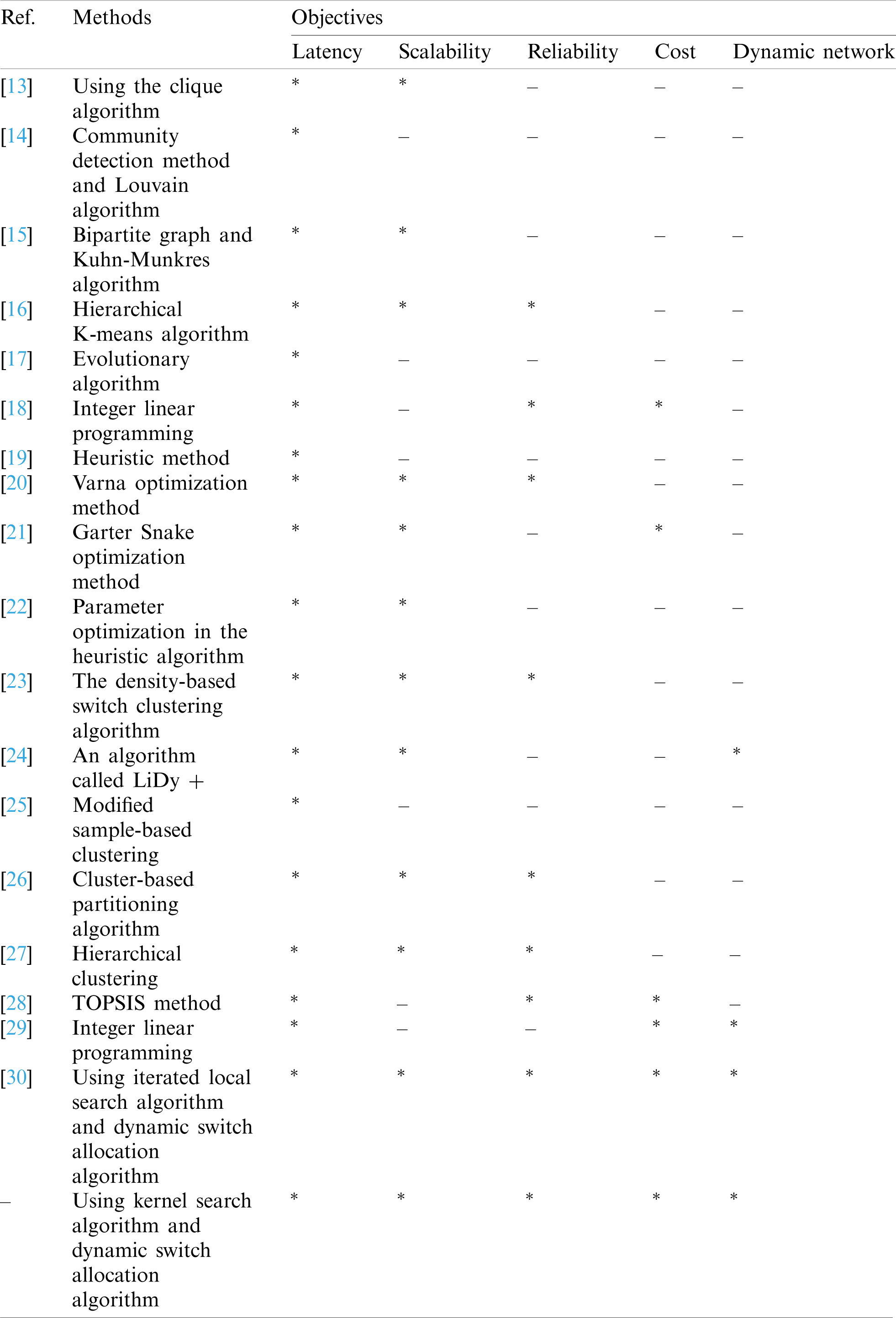
Tab. 1 shows that most of the works focus on latency, reliability, and scalability. Fewer research have focused on cost and network dynamics. Only research work in [30] and latency, reliability, and scalability criteria also focus on cost and network dynamics. Research in this paper extends and improves the work in [30]. Extensive experiments show the significance of the improvement.

3  The Proposed Framework

In this work, we consider the SDN network as a graph. The objective function is multi-objective that also takes into account the cost and survivability. One way to solve multi-objective problems is to turn the objective function into a constraint with multi-objective decision-making techniques. The cost is considered an objective function, and survivability is considered as a constraint in the problem’s mathematical model. We used the kernel search algorithm for the state when the network is in the static state. Then, in the network dynamics state, the dynamic allocation algorithm has been implemented. The scenario used in this paper is as follows:

The graph consists of the locations of the controllers and switches. The switches must be connected to the controllers, and at the controller installation locations, locations are selected as candidates for the controller installation. Graph nodes may form clusters so that there are several controllers in each cluster. From the controllers, one is the cluster head managed by a central controller. The connection of switches and controllers is in-band or out-band. The Controllers, switches, and links each have limitations, including resource constraints, bandwidth constraints, and the amount of data sent, respectively. Each controller processes the load sent by the switches according to its resources. We use the backup controller when the central controller fails. Besides, for link failure, we use disjoint paths.

3.1 The Mathematical Expression of the Problem

Referring to Fig. 2, the network graph consists of nodes V and edges E. V contains switch nodes S and controller nodes P. In other words, V = S ∩ P and S ∩ P = ø.

Figure 2: Network graph with G = (V, E)

Set E also contains two sets of EP and ES such that:

EP={ab∈E|a,b∈P} (1)

ES={ab∈E|a∈S,b∈P} (2)

Other sets include O, and C. O represents ordered pairs of possible locations to install the controller. C indicates the type of controller. In mathematical form:

O={(a,b):a∈P,b∈P,a<b} (3)

C={c1,c2,…} (4)

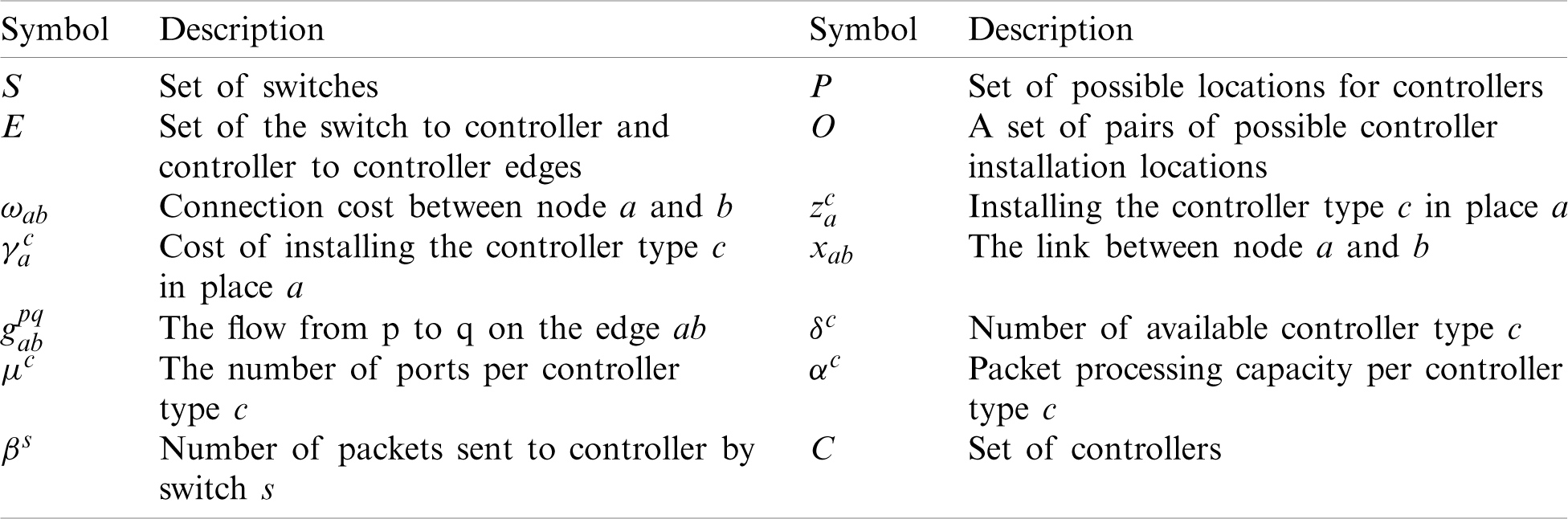
Due to the controller port’s limitations, one controller and the other switches can connect several switches. Also, each controller can communicate with other controllers. Tab. 2 shows the symbols used in the model.

Decision variables:

xab={1If edge (a, b) is selected,0Otherwise,zca={1If a controller of type c is placed in node a,0Otherwise,gabpq={1If a unit flow from location p to location q passes edge (a, b)0Otherwise,

Table 2: Symbols used in the model

Finally, the mathematical model of the problem:

Formulation(1):min∑ab∈Exabωab +∑c∈Cγac∑a∈Pzac∑ab∈EP gabpq−∑ba∈EPgbapq={ ∑c∈C(zpc*zqc)a==p−∑c∈C(zpc*zqc)a==q ∀a∈P, ∀pq∈O0 a≠p,q (5)

∑b∈Pab∈ESxab=1; ∀a∈S (6)

xab≤∑c∈Czbc; ∀ab∈ES, a∈S, b∈P (7)

∑c∈Czac≤1; ∀a∈P (8)

∑a∈Pzac≤δc; ∀c∈C (9)

∑a<bb∈Pxab+∑b∈Sba∈ESxba≤∑c∈Cμc*zac; ∀a∈P (10)

∑b∈Sba∈ESβs*xba≤∑c∈Cαc*zac; ∀a∈P (11)

xab∈{ 0,1 } ∀ab∈E (12)

zac∈{ 0,1 } ∀a∈P,c∈C (13)

gabpq∈{ 0,1 } ∀ab∈EP,∀pq∈O (14)

The objective function represents the minimum costs of connecting network components (switch and controller) and deploying the controller. Constraint (5) indicates the communication between the two controllers. Constraints (6) and (7) indicate that each switch is connected to a controller. Constraint (8) indicates the deployment of only one controller in each location. Constraints (9)–(11) express the controller’s limitations, including the available number, port, and processing capacity.

The expression ∑c∈C(zpc*zqc), in constraint (5), is a nonlinear equation, and to convert it to a linear equation, we do the following:

tpq=∑c∈C(zpc*zqc) (15)

{tpq≤ min(∑c∈Czpc,∑c∈Czqc)tpq≥ max(0,∑c∈Czpc-(1-∑c∈Czqc))∀pq∈O (16)

Or equivalently:

{tpq≤∑c∈Czpctpq≤∑c∈Czqctpq≥∑c∈Czpc-(1-∑c∈Czqc)∀pq∈O(17)

As a result, we have:

Formulation(2):min∑ab∈Exabωab+∑c∈Cγac∑a∈Pzac (5)–(17)

∑ab∈EPgabpq-∑ba∈EPgbapq={tpqa==p-tpqa==q∀a∈P,∀pq∈O0a≠p,q (18)

tpq∈{0,1}∀pq∈O (19)

3.2 The Kernel Search Algorithm

This algorithm [31] is a heuristic used to solve 0–1 program problems, and also used for each Binary Integer Linear Programming (BILP) problem, which is promising binary variables if it equals to 1. All promising variables make up the kernel, and is divided into two types: the private kernel and the public kernel. The former consists of promising variables, and the latter consists of the union of private kernels. Both the private kernel and the public kernel are different.

In the kernel search algorithm [32,33], the original problem’s linear relaxation is first solved. Then the initial private kernels are formed for each variable set. The union of the initial private kernels acquires the initial public kernel. The variables do not contain the initial private kernel, which is categorized into ordered categories, called private buckets. In Algorithm 1, a pseudo-code of the Kernel Search solves the controller placement problem.

In this algorithm, the initial private kernel is based on the answer to the first step. Buckets are made from the smallest to the largest using the reduced cost coefficients. The current private kernel update is as follows. A member variable of the private bucket becomes the current private kernel, which is not considered a promising variable.

BILP (Z, X, V) contains the set of variables representing the controller installation at the location i, the switch and the controller connection, and communication of controllers with each other, respectively. In other words, mathematically:

Z={Zac}∀a∈P,∀c∈C (20)

X={Xab}∀a∈S,∀b∈P (21)

V={Xab}∀a∈P,∀b∈P (22)

The linear relaxation of BILP (Z, X, V) is denoted as LP (Z, X, V). In the kernel search algorithm, the private kernel for the set of X-variables and V-variables should be consistent with the private kernel set of variables Z. The same argument is also used for private buckets.

The private kernel for variables Z, X, and V are represented as K(Z), K(X), and K(V), respectively. Each Zac in K(Z) serves a subset of switches. If Zac values do not exist in K(Z), the variable Xab does not exist in K(X) and K(V). The public kernel is represented by K, obtained from the union private kernels K(Z), K(X), and K(V).

The kernel search algorithm functions in two phases. In the first phase, LP (Z, X, V) is solved. (ZLP, XLP, VLP) indicates the solution to solve the LP problem. If (ZLP, XLP, VLP) is an integer, this value is considered the best solution to the problem, and the algorithm ends. Otherwise, the LP value is considered the lower bound of the objective function, which is used to detect promising variables. Then, the algorithm sorts the set P. For this purpose, the variable Zac reduced cost is obtained from LP, which is indicated by c’(Zac). The positions are then sorted in descending order based on the number of connected switches used in LP (Z, X, V). Places not selected in LP solution, i.e., Zac=0, sorted by ascending order of c’(Zac) values. These sorted values are placed in a list called L. In this list, places to have a controller are first, and the other positions are the last part of the list.

After sorting positions, the switches should be connected to these positions. Therefore, the reduced cost of the variable Xab obtained from the LP solution displayed the symbol c’(Xab). Then, a subset of the switches is connected to the selected positions, with the condition that the value of c’(Xab) for each pair (S, P) must not exceed the threshold value γ. i.e., C′(Xab)≤γ. The value of the parameter γ, obtained from the median of the reduced costs of the variables Xab related to members of the initial private kernel K(Z). i.e.,: γ=median{C′(Xab)|a∈S,b∈K(Z)}.

The created public kernel is called K. The set K(Z) contains m of the variable Zac from the first list L that the value of m is given as the parameter to the algorithm. The K(X) for each member position of K(Z) also contains a subset of the switches associated with that position. The remaining |P| − m positions are classified into NB sets; each set represents as B(Z)h. h takes a value between 1 and NB. B(Z)h=1,…,NB is denoted as private buckets. Each set B(Z)h except for the last set, i.e., h=NB, has the number of lbuck members whose lbuck is equal to the parameter m. The last set has the number of (|P| − m) −((NB −1) * m) members. Thus, according to the contents expressed, the number of buckets can also be calculated with this formula, NB=⌈|P|-mlbuck⌉. Likewise, the NB private bucket creates the variable X, represented as B(X)h=1…,NB. The run algorithm’s maximum number can be considered NB to determine the stopping condition for implementing the kernel search algorithm. Therefore, the NB parameter determines the number of times to run the algorithm.

In this algorithm, the variable zH is used as the upper bound of the BILP problem. Before solving the BILP problem, check that each switch connects at least one set K(Z) position. If the switch is not connected, set K(X) is corrected; through the way, the corresponding switch is connected to all the positions in K(Z) and set K(X) is updated.

In the second phase, the BILP problem along with NB is solved. In each iteration h, where is h = 1, NB, the current public kernel K is updated by adding the member variables of the current private buckets B(Z)h and B(X)h. The BILP problem is solved based on the updated kernel and the definition of two new constraints aiming to reduce computing times. One of these constraints is changing the optimal solution’s upper bound, and another is to select at least one position from the current private buckets to solve the problem. If the BILP problem is feasible, the best solution will be provided according to the ontained optimal solution. In this case, at least one position from its current private bucket is selected in the optimal solution, and the current private Kernel K(Z) updates these variables. The set includes these positions are shown as B(Z)+h.

Conversely, if a position in the current private kernel has not been selected and the number of times t, the variable is not promising, then it is removed from its private kernel. The value of the parameter t in this algorithm is equal to 2. The set, including these positions, is shown as B(Z)−h. Thus, at the end of the iteration h, the current kernel K(Z) at the beginning of iteration h + 1 consists of the members of the set B(Z)+h, and minus the members of the set B(Z)−h. The same procedure is performed for the current private kernel K(X). If a new position is added to the K(Z), the switches associated with the new position are added to the current private kernel K(X). Conversely, when a position is removed from K(Z), the switches associated with that position are removed from the current private kernel K(X). When the last bucket has been evaluated, the algorithm ends.

Fig. 3 shows an iteration of the kernel search algorithm. The black and gray circles represent the initial kernel and buckets at the beginning and end of the first phase, which is BILP (K). At the beginning of the second phase, BILP (K U B1) is considered as a problem. If an optimal solution is obtained, the kernel is updated, i.e., promising variables (empty circles) are added, and variables that are not promising for a long time are deleted from the kernel (cross-references). The second phase continues with solving the BILP (K U B2) that kernel K has been updated.

Figure 3: An iteration of the kernel search algorithm [32]

The algorithm does not work properly in both cases. The first case occurs when there is no feasible solution for LP. The second case occurs when no feasible solution is found for each BILP problem. The latter case occurs while the positions’ capacity to connect the switches associated with it, is not enough. The implementation of the kernel search algorithm depends on the exact determination of the parameters.

In order to examine the complexity of the kernel search algorithm, we consider its execution time. Algorithm execution time is an essential criterion in any algorithm that shows us how long the algorithm takes to complete a given input. One standard method for analyzing the complexity of algorithms is asymptotic analysis. In this method, execution time is calculated according to the size of the input. Since the controller placement problem is to determine the controllers’ number and location and the number of possible locations, P, to install the controller as input to the algorithm is given. Therefore, the complexity of the algorithm depends on the value of P.

As we follow and extend the work in [30], we consider all the conditions mentioned there regarding the events causing the network’s dynamics and failures. Hence, we refrain from stating them again in this section.

4  Experiment and Analysis

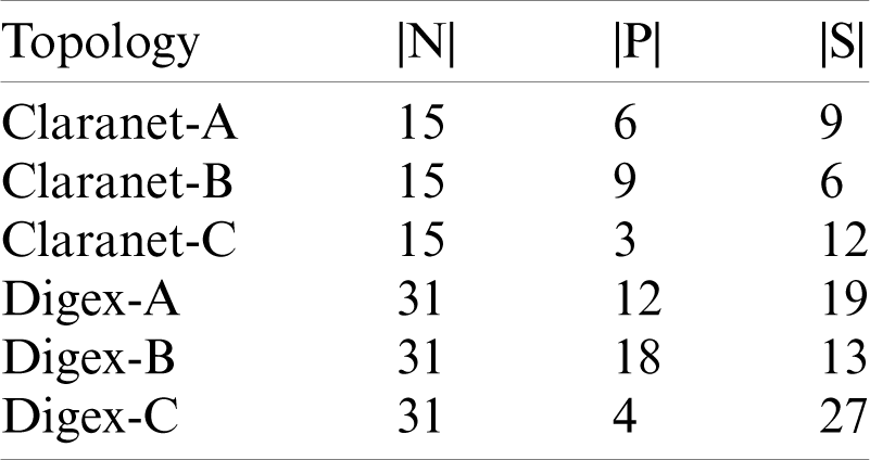
In this section, we have presented the results of the simulation of the proposed framework, which refers to the comprehensive model for controller placement (Section 3.1) and the proposed algorithm (Section 3.2). The is reason is that unlike previous research, the comprehensive model is, to deal with the controller placement problem in more detail and with realistic assumptions. This model comes with the proposed algorithm that can be implemented on any network type, with any size and topology. In order to evaluate our proposed framework, we performed experiments. In these experiments, we compare the proposed framework’s results with EMCPP [29] ILS [30]. To perform these experiments, we select topologies from the Internet Topology Zoo [34]. Tab. 3 shows the information of these topologies.

Table 3: Information of experimented topologies

The experiments were carried out in three steps. First, we evaluated the proposed framework in terms of network cost; then, we examined the network’s survivability. For this purpose, we used formulation (4) defined in [30]. Finally, in the third step, we examined the framework based on connection failure probability and the average delay.

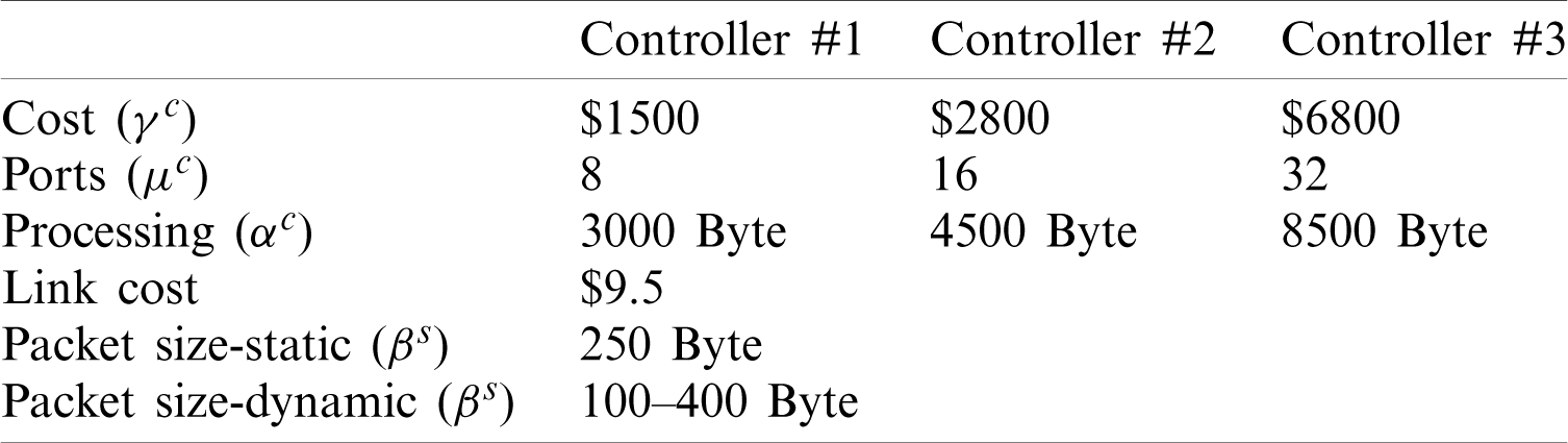
These experiments were performed using a system with Intel Core-i5 processor with 8 GB of RAM. CPLEX and MATLAB software were used to implement the comparison methods. CPLEX is commercial software package and a well-known Branch and Bound solvers of mixed-integer programming problems. Indeed, extensive studies in mathematical programming literature would suggest CPLEX as the most powerful commercial. The parameters used in these experiments are shown in Tab. 4.

Table 4: Experiment parameters

Each experiment was repeated ten times to achieve more accurate results. Tabs. 5 and 6 show the results of these experiments.

Table 5: Comparison of the proposed framework with EMCPP and ILS methods

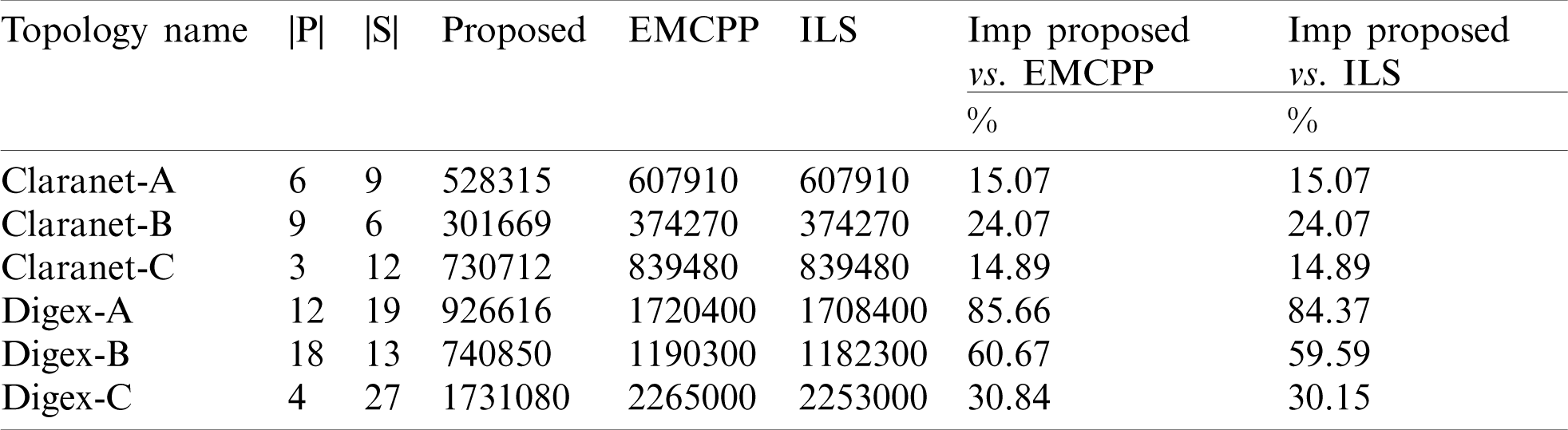
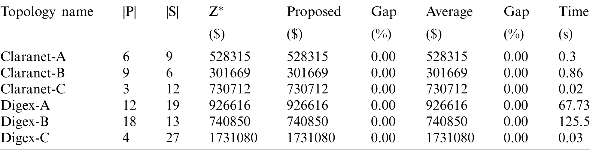
Table 6: Results of the proposed framework

In Tab. 5, the first to third columns show information about the topologies. Columns 4 to 6 show the best cost of the proposed framework and the EMCPP and ILS. The last two columns also express the percentage of improvement of the proposed method compared to EMCPP and ILS, which are calculated by (23) of this percentage.

ProposedorAverage-Z*Z**100(23)

According to the results shown in Tab. 5, it can be concluded that the proposed framework performs better than its counterparts in most of the experimented topologies. This advantage is even more noticeable when the topology size is more extensive. The reason is the proper design of the control plane architecture. The proposed framework designs the control plane in such a way as to reduce the cost of links. Also, survivability remains at a desirable level. However, the methods compared, and used the full mesh topology to connect the controllers. This topology requires many links to connect each controller. Hence, connections impose a high cost on the network. According to the experiments results analysis, at least 67% of the network cost is related to connecting the switch to the controller and the controller to the controller.

The reduction of some topology improvement percentages is related to the topology structure and switches and controllers’ arrangement. For this reason, the controller placement is critical, as the deployment of the switches is random.

The first to third columns in Tab. 6 show information about the experimented topologies form which Z* indicates the best solution for each topology, and the fifth column focuses on the proposed framework for a solution. The Gap expresses the deviation of the best solution, which is calculated by (24).

CostEMCPPorILS-CostproCostpro*100(24)

The average column is the mean of the best solution with ten times runs. The eighth column shows the deviation of this average. The time column expresses the average execution time of the algorithm.

The results related to the network’s survivability are shown in Figs. 4 and 5. In these Figures, R indicates the degree of survivability. The proposed framework is more cost-effective in terms of network survivability in the event of a failure. Thus, the proposed framework receives a higher degree of survivability than the methods compared. The EMCPP does not provide any flexibility in selecting the required survivability. At the same time, the proposed framework receives the required survivability as input. Therefore, a different amount of survivability can be imposed on different network based on user observations. According to these experiments’ results, the proposed framework imposes a lower cost on the network both in terms of implementation and survivability. Also, the proposed framework includes the proper use of ports. Despite applying a complete graph to the installed controllers, each controller needs to connect to other controllers in the full mesh topology, a port occupation. Experiments show that using such a topology imposes a high cost on connecting controllers to the network. This does not show a balance between the various costs of the objective function.

In contrast, the proposed framework usually finds the best balance between the objective function’s different costs. Even the EMCPP cannot guarantee a high degree of survivability for cases where a small number of controllers are installed. For example, when only two controllers are installed, there is only one connecting link between the two controllers, and there is no guarantee that the link does not fail. Therefore, paying attention to the control plane architecture is essential to solve the controller placement problem.

Figure 4: Comparison of experiment results on Claranet topology (a) Claranet-A (b) Claranet-B (c) Claranet-C

As shown in Fig. 4, the proposed framework costs less for different R values than the EMCPP and ILS for the Claranet topology. In Fig. 4c, there is no answer for R = 3 because, in topology Claranet-C, |P| = 3. Hence, for R = 3, we need |P| = 4.

Figure 5: Comparison of experiment results on Digex topology (a) Digex-A (b) Digex-B (c) Digex-C

Fig. 5a shows that the proposed framework’s cost with R = 2 and R = 3 costs less than EMCPP and ILS with R = 1. Also, in Fig. 5b, the proposed framework’s cost with R = 2 and R = 3 is lower than EMCPP and ILS with R = 1 and R = 2, respectively. i.e., the cost of the proposed framework for R = 2 is 1063660, while the cost of EMCPP and ILS for R = 1 is 1190300 and 1182300, respectively. This means that the proposed framework, compared to the EMCPP and ILS, can design a network that increases survivability while reducing cost. Finally, it can be concluded that the proposed framework is more cost-effective for large-scale networks than the EMCPP and ILS, even when the degree of survivability increases compared to the EMCPP and ILS.

One of the proposed framework’s main advantages is that the network’s survivability can change dynamically depending on the network’s environment, and affecting the cost of network implementation. For example, networks with secure environments do not require a high degree of survivability. Hence, the cost can also be reduced if a full-mesh topology in the control plane architecture design for secure environments incurs additional costs. The proposed framework focuses on network dynamics such as increasing or decreasing switches and controllers, making it stand out. Another advantage of the proposed framework is using a kernel search algorithm to find the best solution in the shortest time.

4.1 Connection Failure Probability

The connection failure probability includes the probability of controller failure and the probability of the link failure. To compute the link failure probability, we considered link disruption probability (PLD) and link congestion probability (PLC). Eqs. (25) and (26) were used for this calculation:

PCF=1k∑a=1k[Pa(r)+∑b=1,b≠an(PLD(eab)+PLC(eab))] (25)

P(r)=∏i=1MP(r|h,e,l,p) (26)

e, l, h, p, and r, respectively, indicate the probability of environmental, link, hardware, power failure, and the installed controller’s reliability index. PLD (eab) and PLC (eab) calculated using (27) and (28). The variable k indicates the number of subdomains. The subdomains were obtained according to the segmentation of the network.

PLD(eab)={dab.pulyabyab=1∞yab=0(27)

In (27), PLD (eab) indicates the probability of link disruption between a and b. dab and yab indicate the distance between a and b and the connection link between these two nodes, respectively. pul also indicates the probability of link failure per unit length. In these experiments, the value of pul was obtained for every 1 km.

PLC(eab)={χab.λa+χba.λbyab.ωabyab=1∞yab=0(28)

In (28), the PLC (eab) indicates the probability of link congestion between a and b. χab and ωab indicate the traffic direction and link bandwidth, respectively. If the traffic direction is from a to b, then χab=1; otherwise, χab=0. λa shows the flow request rate of the switch a.

Now, in particular, by selecting two topologies Claranet-A and Digex-A, we examined the probability of connection failure. The result of this experiment is shown in Fig. 6.

Figure 6: The probability of connection failure (a) Claranet-A (b) Digex-A

For this reason, in the case of failure in the communication link, the probability of connection failure is maximized. EMCPP and ILS consider the shortest path between nodes, thus preventing disconnection of some connections. Given that the reliability rate is considered in the proposed method, it can reduce connection failure.

4.2 The Average Delay

This delay consists of the propagation dprop, the processing dproc, and the transmission dtran delays. In this experiment, the values of dproc = 0.01 ms and dtran = 0.05 ms are considered. Also, the value of dprop increases by 0.1 milliseconds for every 1 km. Accordingly, by changing the number of controllers, we calculate each method’s average delay for the two topologies Claranet-A and Digex-A. The results of this experiment are shown in Figs. 7a and 7b.

Figure 7: The average delay (a) Claranet-A (b) Digex-A

As shown in Figs. 7a and 7b, adding a controller in all three frameworks causes to decrease the average latency. The proposed method performs better in reducing latency compared to the other two methods. This reduction is due to the reliable controller placement, proper distribution of switches, and the delay when allocating the switch to the controllers. Therefore, the average delay has significant decrease. When the number of controllers reaches higher than 8, the delay is relatively stable.

5  Conclusion

Two metrics of cost and survivability as factors affecting the control plane’s efficiency and the network’s overall efficiency were examined in this paper, as in the related works, these criteria have not received adequate attention from researchers. Since minimizing the cost is one of the influential factors in network implementation, it is essential to consider this criterion in solving the controller placement problem. As shown in the simulation results, 67% of the costs are related to connecting network elements to each other. Therefore, improper location of controllers can increase the cost of network implementation. As for the survivability criterion, since networks are at risk in real environments, solutions must be considered for the network’s stability in these events. Therefore, paying attention to this criterion also has a significant effect on solving the controller placement problem. Then, the mathematical model of the problem was presented to take into account the stated criteria in which the cost was considered as an objective function and survivability as a constraint. As the controller placement problem space becomes larger as the network size increases, an algorithm is needed to get the best solution in the shortest time. For this purpose, the kernel search algorithm was used in the controller placement problem. Then, to check the accuracy of the proposed mathematical model and the proper performance of the proposed algorithm, by performing simulations, a comparison was made with the EMCPP and ILS based on cost and survival criteria. In this simulation, six different topologies of the Internet topology Zoo were selected to evaluate the proposed framework’s performance. The state of the network was also examined in terms of dynamics and events that cause network failure. The results obtained in the network’s dynamic state showed that the proposed framework has a better performance in reducing costs and increasing the network’s survivability. Thus, the proposed framework has a 38.53% and 38.02% improvement in reducing network implementation costs than EMCPP and ILS, respectively. Therefore, the summary of these results indicates that the proposed framework, using a suitable mathematical model close to the actual network conditions and an algorithm with the best speed of action to find the best solution, can solve the controller placement problem.

We will try to solve the controller placement problem with traffic forecasting based on machine learning in future work. We also plan to expand our work in the future by addressing the dynamic controller placement to meet the needs of 5G networks, such as reliable low-latency communications.

Funding Statement: The authors received no specific funding for this study.

Conflicts of Interest: The authors declare that they have no conflicts of interest to report regarding the present study.

This work is licensed under a Creative Commons Attribution 4.0 International License, which permits unrestricted use, distribution, and reproduction in any medium, provided the original work is properly cited.