DOI:10.32604/cmc.2021.017633
| Computers, Materials & Continua DOI:10.32604/cmc.2021.017633 | |
| Article |
UFC-Net with Fully-Connected Layers and Hadamard Identity Skip Connection for Image Inpainting
1Korea Electronics Technology Institute, Seongnam, 13488, Korea
2School of Electrical Engineering, Korea University, Seoul, 02841, Korea
*Corresponding Author: Eenjun Hwang. Email: ehwang04@korea.ac.kr
Received: 01 February 2021; Accepted: 05 March 2021
Abstract: Image inpainting is an interesting technique in computer vision and artificial intelligence for plausibly filling in blank areas of an image by referring to their surrounding areas. Although its performance has been improved significantly using diverse convolutional neural network (CNN)-based models, these models have difficulty filling in some erased areas due to the kernel size of the CNN. If the kernel size is too narrow for the blank area, the models cannot consider the entire surrounding area, only partial areas or none at all. This issue leads to typical problems of inpainting, such as pixel reconstruction failure and unintended filling. To alleviate this, in this paper, we propose a novel inpainting model called UFC-net that reinforces two components in U-net. The first component is the latent networks in the middle of U-net to consider the entire surrounding area. The second component is the Hadamard identity skip connection to improve the attention of the inpainting model on the blank areas and reduce computational cost. We performed extensive comparisons with other inpainting models using the Places2 dataset to evaluate the effectiveness of the proposed scheme. We report some of the results.
Keywords: Image processing; computer vision; image inpainting; image restoration; generative adversarial nets
Image inpainting is one of the image processing techniques used to fill in blank areas of an image based on the surrounding areas. Inpainting can be used in various applications, such as image/video uncropping, rotation, stitching, retargeting, recomposition, compression, super-resolution, and harmonization. Due to its versatility, the importance of image inpainting has been particularly addressed in the fields of computer vision and artificial intelligence [1–3].
Traditional image inpainting methods can be classified into two types: diffusion-based and patch-based methods [4–9]. Diffusion-based methods use a diffusion process to propagate background data into blank areas [4–7]. However, these methods are less effective in handling large blank areas due to their inability to synthesize textures [4]. Patch-based methods fill in blank areas by copying information from similar areas of the image. These methods effectively restore a blank area when its ground truth is a regular and similar pattern. However, they could have difficulty reconstructing an erased area when the ground truth has a complex and irregular pattern [8,9]. As a result, both types of methods have difficulty reconstructing specific patterns, such as natural scenes and urban cityscapes [10].
Recently, deep neural network (DNN)-based methods [11–15] have significantly improved image inpainting performance compared to diffusion-based and patch-based methods. Generally, because DNN-based methods fill in the blank areas using learned data distribution, they can produce consistent results for blank areas, which has been almost impossible using traditional methods. Among the DNN-based methods, adapting the generative adversarial network (GAN) has become mainstream for image inpainting [11,16]. The GAN estimates the distribution of training data through adversarial training between a generator and discriminator. Based on this distribution, the GAN reconstructs the blank area realistically in inpainting [11–15,17]. Still, this approach often produces unexpected results, such as blurred restorations and unwanted shapes, when the image resolution is high, or the scene is complex [10,11,13].
One plausible approach to solving these shortcomings is to consider spatial support [12]. Spatial support represents the pixel range within the input values necessary to generate one pixel inside blank areas. To fill blank areas effectively, the inpainting model should consider the entire area outside the blank areas. For instance, Iizuka et al. [12] proposed a new inpainting model using dilated convolutions to increase the spatial support from
In this paper, we propose a new inpainting model called UFC-net using U-net with fully connected (FC) layers and the SC. The proposed model is quite different from other models from two perspectives. First, UFC-net allows full spatial support, which recent inpainting models cannot guarantee [12–15]. Second, UFC-net uses the Hadamard identity skip connection (HISC) to reduce the decoder’s computational overhead and focus on reconstructing blank areas. We first perform qualitative and quantitative comparisons with recent inpainting models to verify that these two differences improve inpainting performance. Then, we demonstrate through experiments that HISC is more effective than the SC in inpainting.
This paper is organized as follows. Section 2 reviews the related work, and Section 3 describes UFC-net and HISC. Section 4 presents the quantitative and qualitative results by comparing UFC-net with several state-of-the-art models. We also quantitatively and qualitatively compare the inpainting performance of the HISC and SC. Section 5 concludes this paper and highlights some future plans.
Three approaches improve the performance of DNN-based inpainting models. The first is to consider spatial support [11,12,14]. The second is to use the SC [18–22], and the third is to improve the restoration performance using some additional techniques, such as loss functions [23–25], a two-stage model [13,15,23,26], and optional input [15,19]. Fig. 1 lists various inpainting models according to this classification.
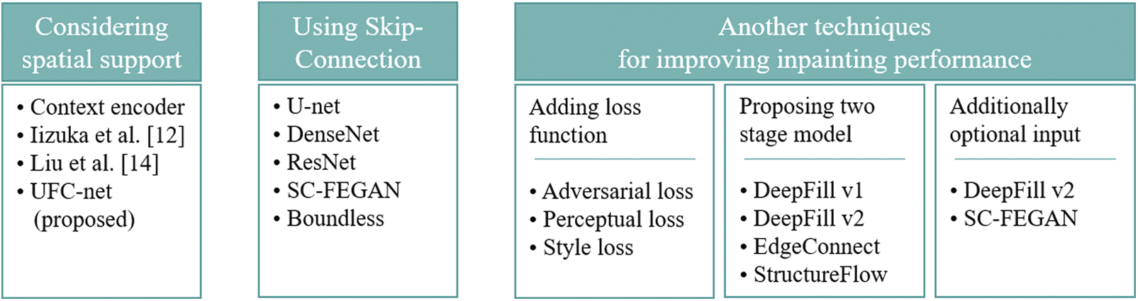
Figure 1: Classification of deep learning-based inpainting models
2.1 Considering Spatial Support
The CE was the first DNN-based inpainting model to use the GAN [11]. The CE comprises three components: an encoder based on AlexNet [27], a decoder composed of multiple de-convolutional layers [28], and a channel-wise FC layer connecting the encoder and decoder. Although CE can reduce restoration errors, it cannot handle multiple inpainting masks or high-resolution images wider than
To mitigate these problems, Iizuka et al. [12] proposed a new model consisting of an encoder, four dilated convolutional layers [29], and a decoder. The encoder downsamples an input image twice, and the decoder up-samples the image to its original size. Due to the dilated convolution, their model considered a wider surrounding area to generate a pixel than the vanilla convolution [30]. They called this spatial support and demonstrated that this could extend the area from
Liu et al. [14] applied U-net [20] for both inpainting irregular masks and increasing the region of spatial support. Although their model exhibited more consistent inpainting performance than Iizuka’s model or CE, its spatial support was not sufficient for filling in both regular and irregular masks.
The SC has been studied to address three main problems arising from the training of the DNN: the effect of weakening input values, vanishing or exploding gradients, and performance degradation with increasing network depth. The SC was used in U-net to enhance the effects of input values in image segmentation. DenseNet [21] attempts to mitigate both vanishing or exploding gradient problems and weakening input value effects by connecting the output of each layer to the input of every other layer in a feed-forward network. He et al. [22] suggested and implemented a shortcut connection in every block in the model to alleviate degradation when the network depth increases. Boundless [18] and SC-FEGAN [19] used the SC to provide spatial information, improving inpainting performance compared to each model without the SC. However, in [15], the authors suggested that the SC is not effective when blank areas are large.
2.3 Other Techniques for Improving Inpainting Performance
The extra loss function can be used to improve inpainting performance. For instance, adversarial loss can be used as a reasonable loss function to estimate the distribution and generate plausible samples according to the distribution [11,31]. Following this, adversarial loss has become one of the most important factors in DNN-based inpainting models [12–15]. Additionally, several recent studies on inpainting [13,15,23] have attempted to reduce the frequency of undesired shapes that have often occurred in inpainted data by using perceptual loss [24] and style loss [25].
Alternatively, two-stage models have been proposed to improve reconstruction performance [13,15]. In the first stage, the models usually restore blank areas coarsely by training the generator using reconstruction loss. Then, in the second stage, they restore blank areas finely by training another generator using reconstruction loss and adversarial loss. DeepFill v1 [13] is a two-stage inpainting model in which a contextual attention layer is added to the second generator to improve inpainting performance further. The contextual attention layer learns where to borrow or copy feature information from known background patches to generate the blank patches. Yu et al. [15] proposed a gated convolution (GC)-based inpainting model, DeepFill v2, to improve DeepFill v1. This model created soft masks automatically from the input so that the network learns a dynamic feature selection mechanism. In the experiment, DeepFill v2 was superior to Iizuka’s model, DeepFill v1, and Liu’s model, but some filled areas were still blurry [19].
Nazeri et al. [23] proposed another two-stage inpainting model called EdgeConnect. This model was inspired by a real artist’s work. In the first stage, the model draws edges in the given image. In the second stage, blank areas were filled in based on the results of the first stage. Although the model exhibits higher reconstruction performance than Liu’s model and Iizuka’s model, it often fails to reconstruct a smooth transition [32]. StructureFlow [26] follows the two-stage modeling approach. The first stage reconstructs the edge-preserved smooth images, and the second stage restores the texture in the output of the first stage as the original. StructureFlow is very good at reproducing textures but sometimes fails to generate plausible results [33].
Lastly, inpainting performance can be improved using additional conditions as an input. For instance, DeepFill v2 allows the user to provide sparse sketches selectively as conditional channels inside the mask to obtain more desirable inpainting results [15]. In SC-FEGAN, users can input not only sketches but also color. Both DeepFill v2 and SC-FEGAN are one step closer to interactive image editing [19].
In this section, we present details of the proposed model, UFC-net, including the discriminator, loss function, and spatial support. We first describe the effects of the FC layers in an inpainting model and then introduce UFC-net in detail. Afterward, we discuss the discriminator and loss function for the training process.
3.1 Effects of Fully Connected Layers
Unlike other recent inpainting models, we appended FC layers into the inpainting model to achieve two effects [12–15,19]. The first effect is that the model has enough spatial support to account for all input areas, and the second is that the model can provide sharp inpainting results. We explain these two effects in turn.
The FC layer is connected to all areas for the model to account for all surrounding areas. Recent inpainting models [12–15], which are composed only of convolutional neural networks (CNNs), cannot consider all input areas. For a more detailed explanation, we demonstrate the difference between the U-net model, which is popularly adopted as an inpainting model [14,19], and the U-net model with FC layers.
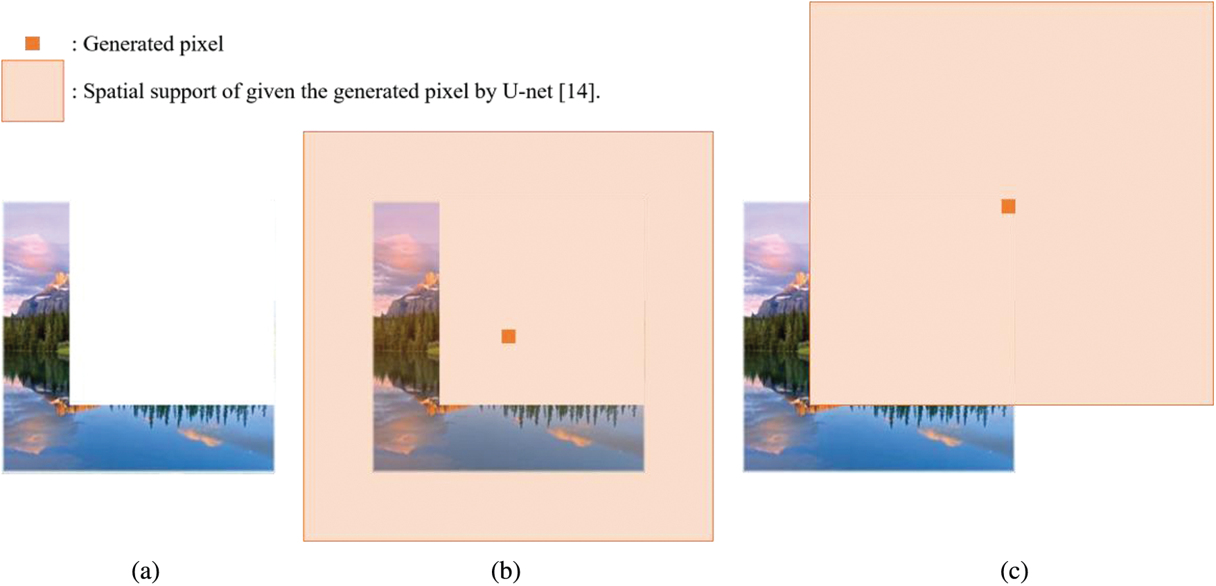
Figure 2: A data sample with a vertex-aligned
For example, for the
Fig. 2b illustrates the case where the spatial support can consider the surrounding area. In contrast, Fig. 2c depicts the case where the spatial support cannot consider any surrounding image even though the spatial support is the same size. In this case, the U-net model fills the blank area regardless of the surrounding area because CNN-based models, such as U-net, construct spatial support with the pixel as the center point.
Unlike the original U-net, U-net with an FC layer can consider all input areas because the FC layer uses all inputs to calculate the output. As a result, inpainting models based on the U-net with FC layer recover all blank regions more effectively by considering all surrounding areas regardless of the position of the generated pixel, as displayed in Figs. 3b and 3c.
Another effect of the FC layer is to naturally transform the input image distribution, including blank areas, into the original image distribution without any blank areas. As typical convolutions operate with the same filters for both blank and surrounding areas, several problems, such as color discrepancy, blurriness, and visible mask edges, have been observed in CNN-based inpainting models [14,15]. Kerras et al. [34] reported that applying the FC layer makes it easier for the generator to generate plausible images because the input distribution is flexibly modified to the desired output distribution. They also revealed that an inpainting model without an FC layer often fails to generate plausible images.
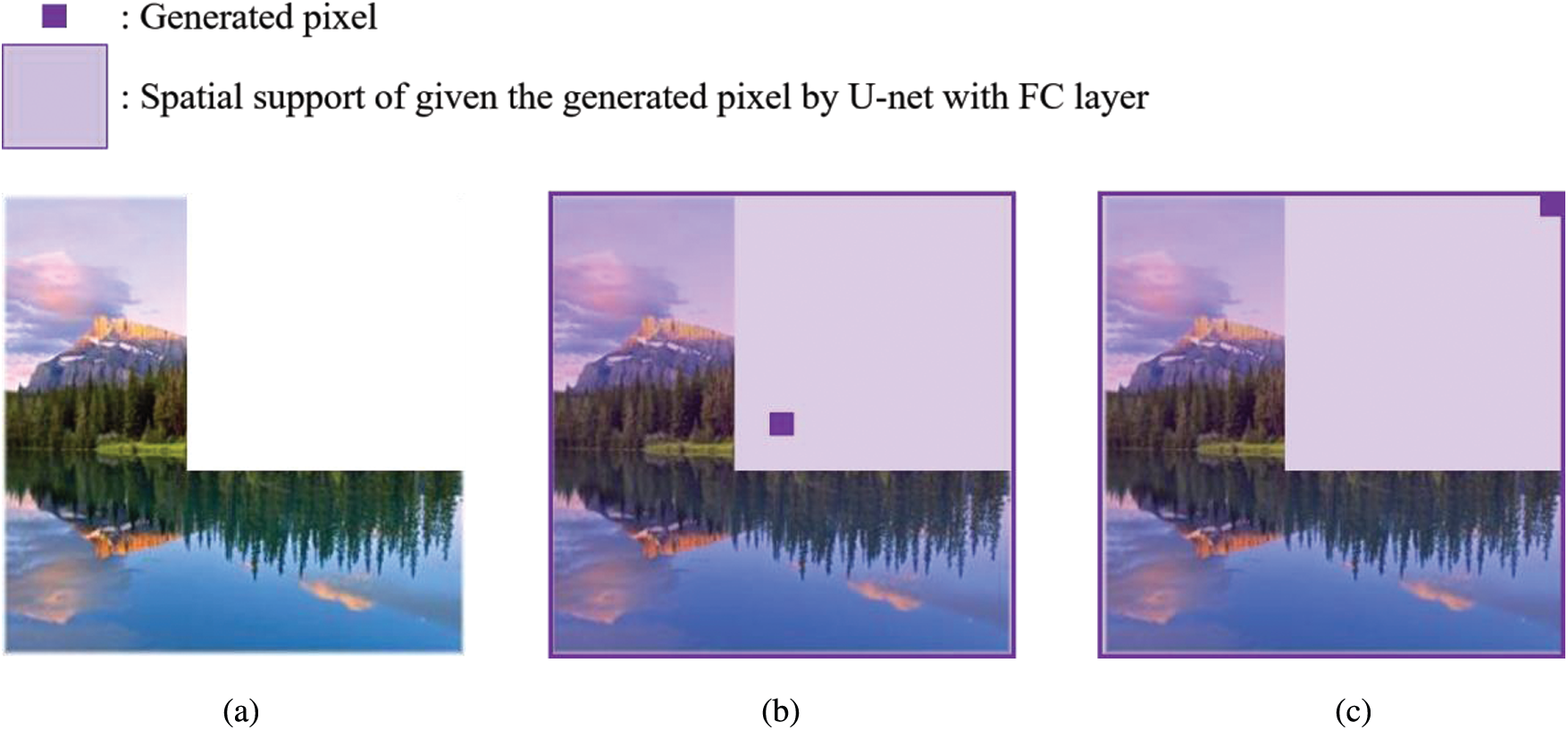
Figure 3: An image sample with a vertex-aligned
Although partial convolution (PC) and GC can alleviate typical convolution problems, they have their limitations. For instance, if the layer becomes deep, PC becomes insensitive to the erased area [15], or two convolutions must be performed in GC. In contrast, the FC layer enables the inpainting model to mitigate the typical convolution problems in inpainting and avoid problems by PC or GC. The FC layer is a trainable weight that can learn both the blank and surrounding areas, which PC cannot do. In addition, inpainting models based on the U-net with an FC layer is lighter than GC-based inpainting models.
We constructed an inpainting model called UFC-net that implements FC layers into U-net to employ the benefits of the FC layer in inpainting. Fig. 4 presents the overall architecture of UFC-net, which has fully spatial support and can transform the input distribution into the original image distribution naturally. The generator model receives masked images, masks, and sketches as input data, where the sketches are optional. A DNN-based generator usually has the risk that the gradient used for learning may disappear [25–27], so the generator in the UFC-net uses batch normalization [35] except for the last layer.
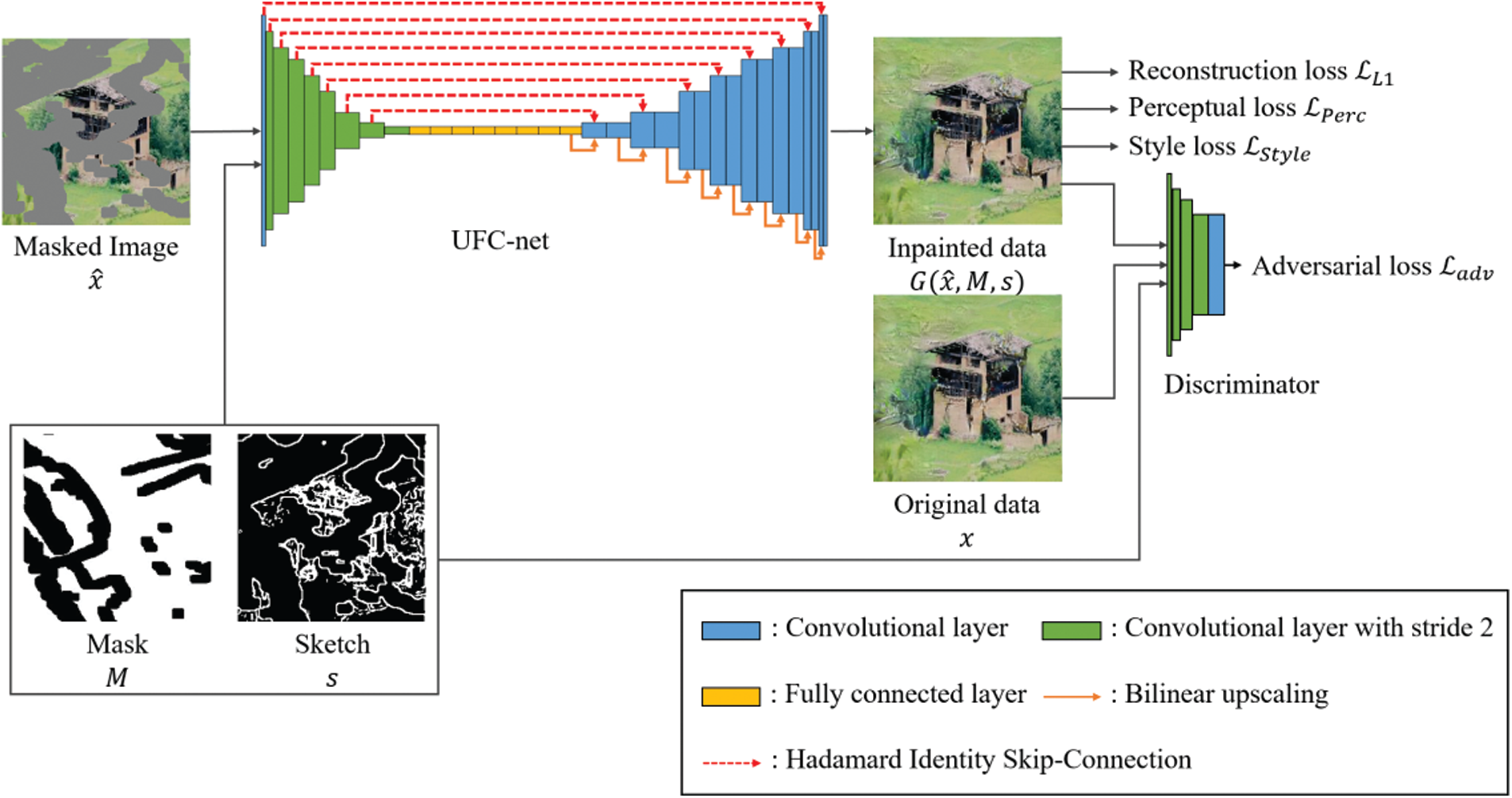
Figure 4: The UFC-net architecture
Table 1: Hyperparameters of the UFC-net encoder
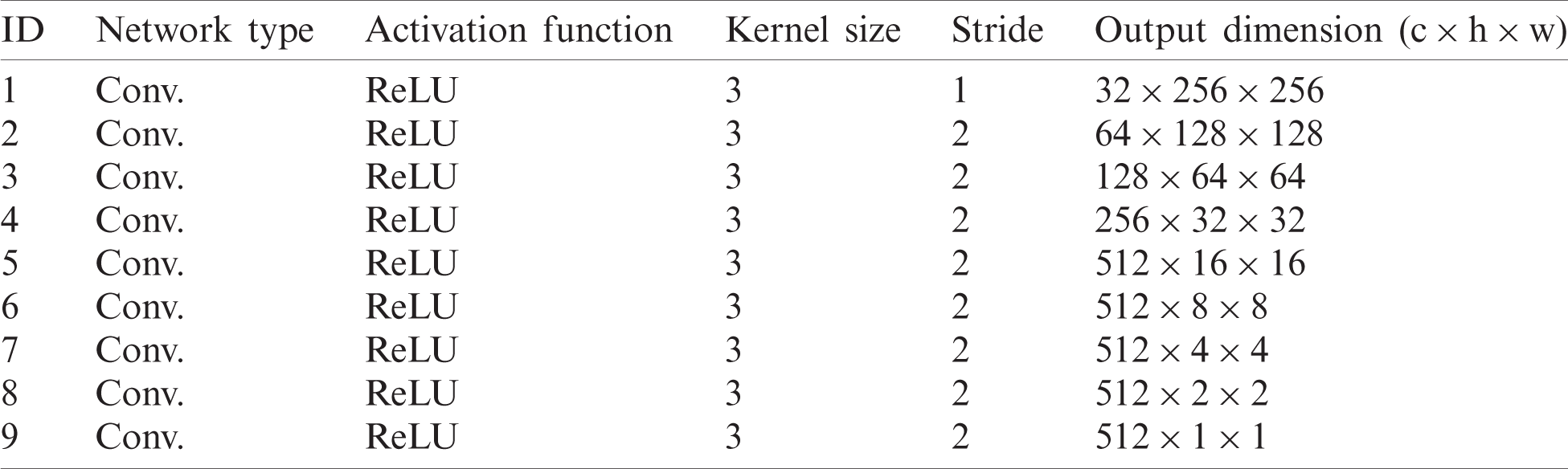
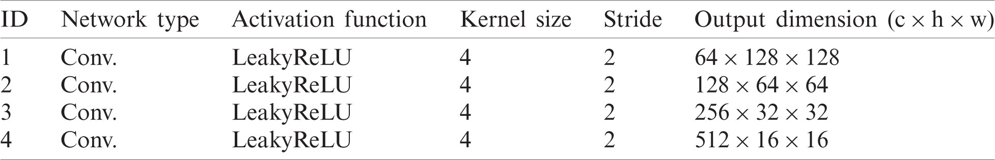
The UFC-net consists of three components: the encoder, latent networks, and decoder. The encoder consists of nine convolutional layers that compute feature maps over input images with a stride of 2. Tab. 1 describes some encoder details.
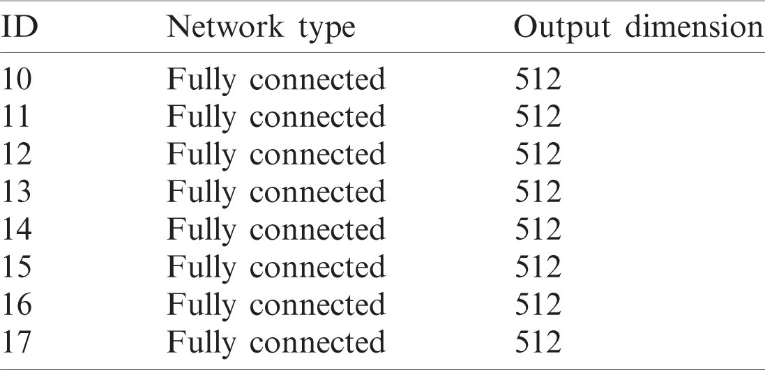
After the encoding process, encoded features pass through eight FC layers to smoothly transform the input distribution to the corresponding output distribution. Tab. 2 presents some hyperparameters of the latent networks in the generator model.
Table 2: Hyperparameters of latent networks in UFC-net
The decoder consists of eight Hadamard identity blocks (HIB). Fig. 5 presents the difference between U-net’s SC and HIB. A typical SC takes the latent value of the encoder and concatenates it channel-wise to the decoder. In the case of HIB, however, the value of the nonblank area is replaced by the latent value of the encoder. The HISC can be defined by Eq. (1):
where
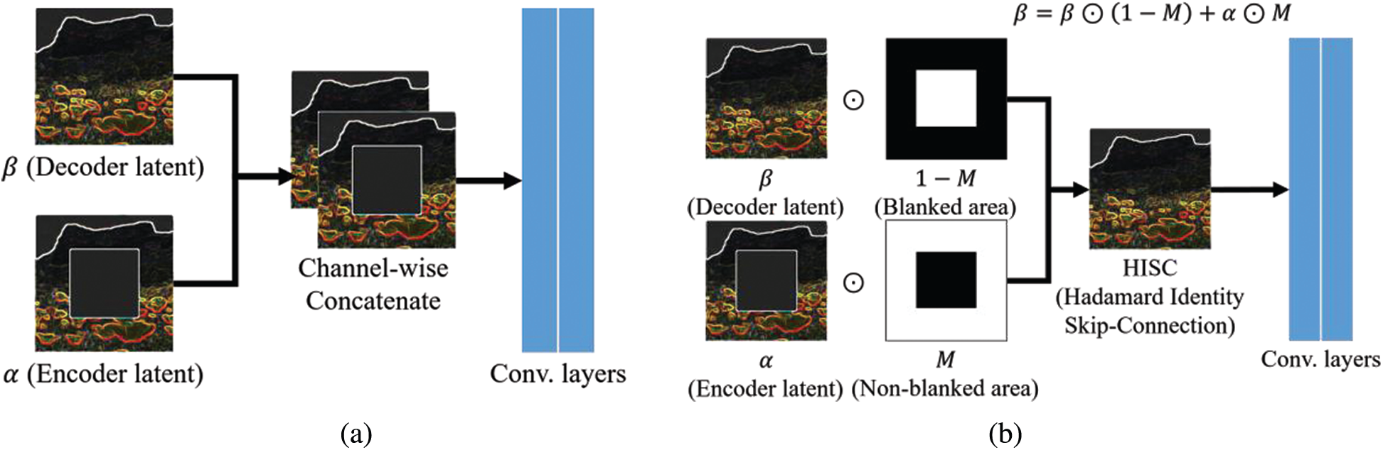
Figure 5: Two convolutional neural networks with skip connections (SC): (a) SC and a couple of convolutional layers, and (b) Hadamard identity block
Table 3: Hyperparameters of decoder networks in UFC-net
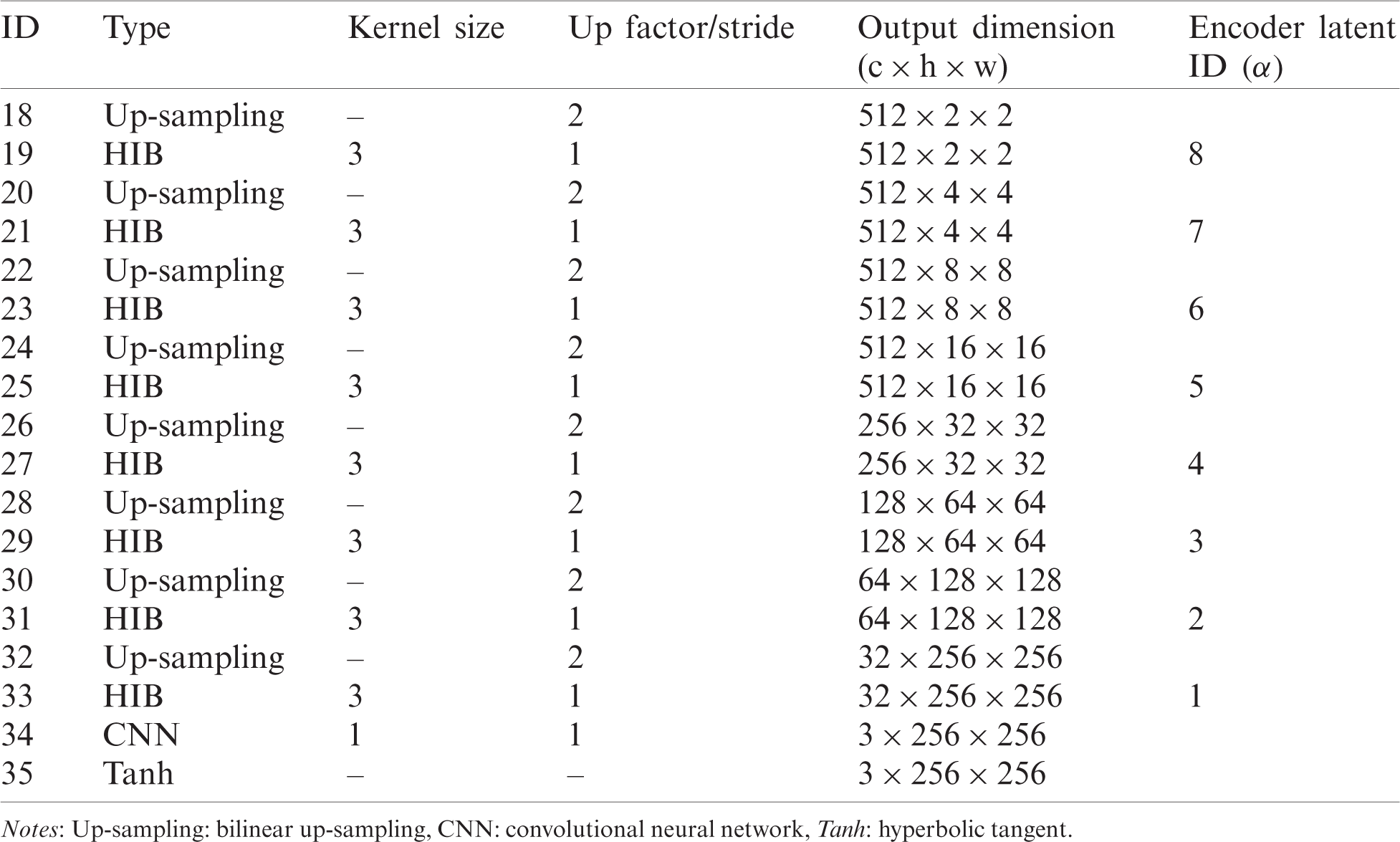
As HISC replaces the decoder latent value with the encoder latent value for nonblank areas, the gradient between the HIB and another HIB is not calculated in these regions. Thus, the HISC reduces the computational cost by having the generator focus on the erased area. Tab. 3 lists some hyperparameters of decoder networks in the UFC-net.
3.3 Discriminator and the Loss Function
Many inpainting models have used the patchGAN discriminator [36] as their discriminator [12–14,23]. However, due to the adversarial training process in the GAN, GAN-based inpainting models often exhibit unstable training [34,37,38]. This problem should be addressed to use the discriminator in GAN-based models. Further, spectral normalization has the property that the generated data are quite similar to the training data [37]. Therefore, we applied spectral normalization to the patchGAN discriminator and used the outcome as the discriminator of UFC-net. Tab. 4 presents the hyperparameters of the patchGAN discriminator.
Table 4: Hyperparameters of the patchGAN discriminator
We used reconstruction loss, adversarial loss, perceptual loss, and style loss to train our model. Reconstruction loss is essential for image reconstruction and is defined using Eq. (2). We used the hinge loss from [15] as the adversarial loss. The adversarial loss effectively restores the results sharply [11,12], which can be defined by Eq. (3). Both perceptual loss and style loss are used to mitigate unintended shapes [14,23], defined by Eqs. (4) and (5), respectively:
where x,
To evaluate the inpainting performance of the proposed model, we conducted various experiments. We first present the environment and hyperparameters for the experiments and then describe the effectiveness of the spatial support and HISC used in UFC-net. In addition, we demonstrate the effect of the sketch input in the proposed model.
As the dataset for the experiments, we used the Places2 [17] dataset, which contains 18 million scene photographs and their labeled data with scene categories. Fig. 6 presents some of the images in the dataset.
We employed two types of masks for training: regular and irregular masks. Regular masks were square with a fixed size (25% of total image pixels) centered at a random location within the image. Irregular masks used the same dataset as Liu et al. [14]. We applied the canny edge algorithm [39] to the Places2 dataset to obtain the sketch dataset. Before training, all weights in the generator and discriminator were initialized with samples of a normal random distribution.
The distribution had 0 for the mean and 0.02 for the standard variation. For training, we used Adam [40] as the optimizer. They were implemented based on the TensorFlow framework and run on Nvidia GTX 1080ti and Nvidia RTX Titan, with batch sizes of 4 and 8, respectively. Both generators and discriminators set the learning rate to 0.002, with one million training iterations. We updated the generator weights twice after updating the discriminator weights once [41].
The proposed model’s primary goals are to widen the spatial support and restore the blank areas for more effective inpainting. Therefore, for comparison, we considered three models that are closely related to these two properties. The models are DeepFill v1 [13], Liu et al. [14] model, and DeepFill v2 [15].
In addition, we used the L1 loss, L2 loss, total variation (TV) loss [14], and variation as the evaluation metrics, which can be defined by Eqs. (7)–(10) as follows:
where R is the region of one-pixel dilation of the hole region, y is
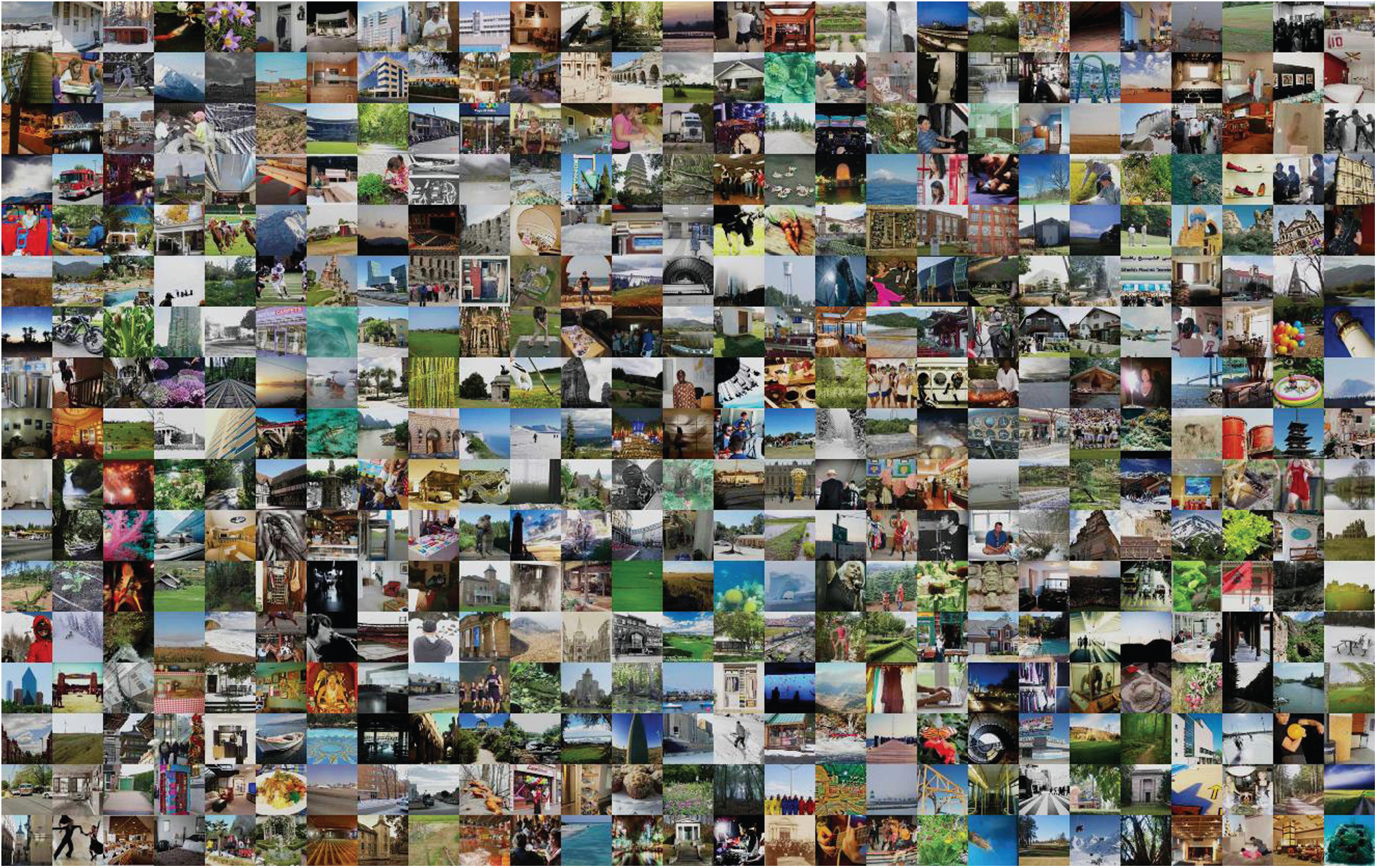
Figure 6: Images from the Places2 dataset
The L1 loss is also known as the least absolute error that measures the absolute difference between the target and estimated values. Similarly, the L2 loss is used to measure the sum of the square of the difference between the target and estimated values. These two loss functions are often used to evaluate the performance of inpainting models. Smaller values of these metrics indicate better generative performance. The TV loss is a metric that expresses the amount of change from the surrounding area based on each pixel for the L1 error. If the TV loss is low, the error does not change rapidly, making it difficult to detect the error visually. The variance indicates the gap performance between the L1 loss and L2 loss in each model. Tab. 5 presents the L1 loss, TV loss, L2 loss, and variance of four models for both regular masks and irregular masks. The proposed model presented the lowest L1 and TV loss errors, which indicates that our model outperforms PC or GC in handling blank areas. However, the proposed model could not achieve the lowest L2 loss and variance. Nevertheless, the proposed model yields the best inpainting results for the human eye. We demonstrate this in the next section.
Table 5: Inpainting implementation of quantitative results. Bold indicates the smallest value (smaller is better) when comparing models in each evaluation metric
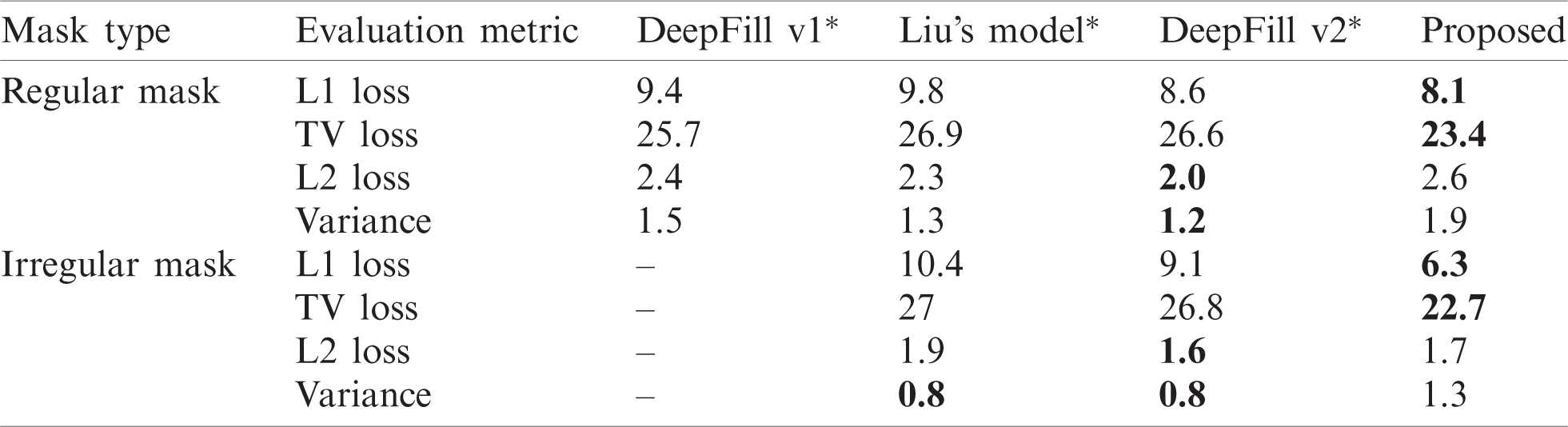
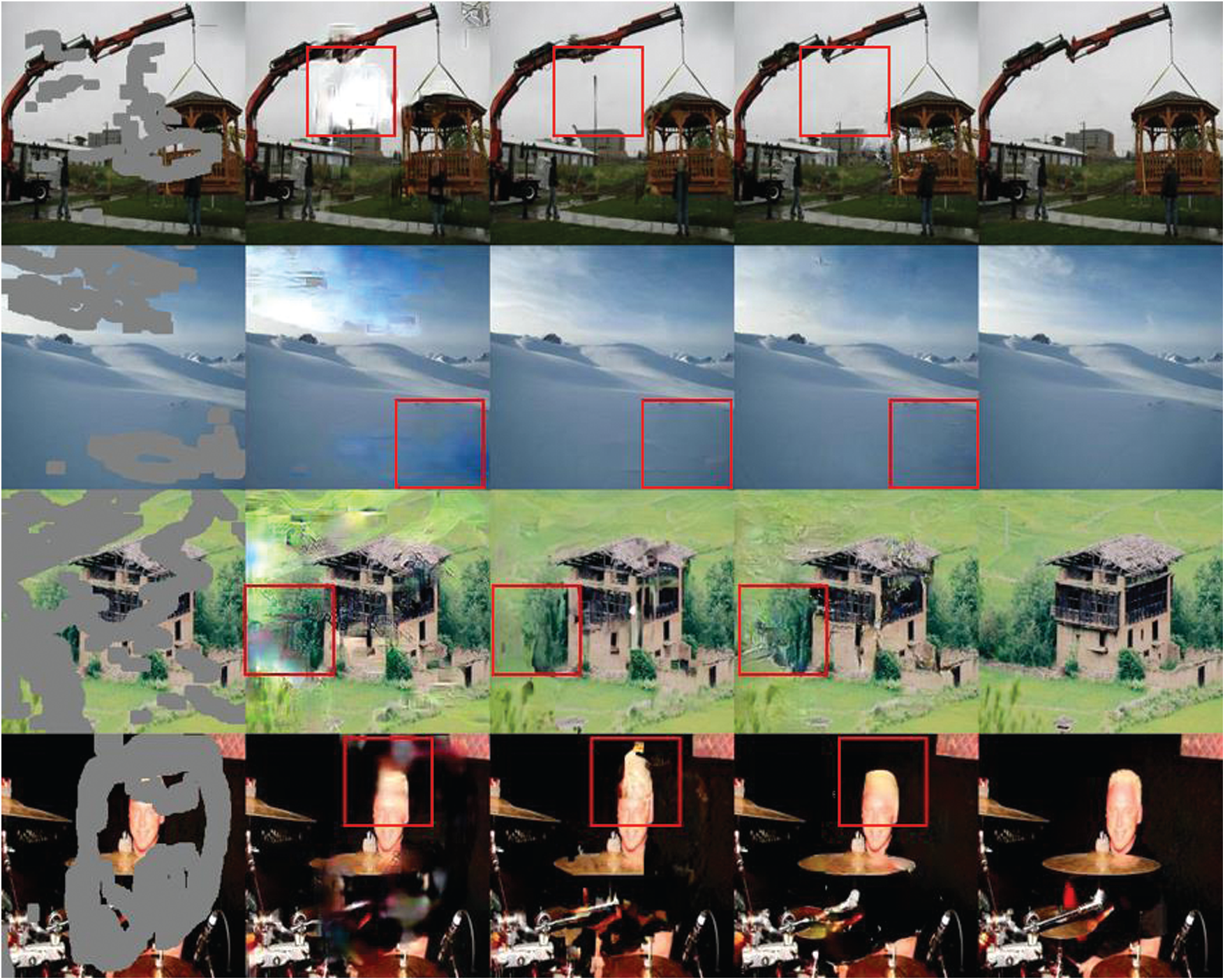
Figure 7: Comparison of inpainting results for the Places2 test dataset
Table 6: Accuracy comparison of HISC and SC in inpainting
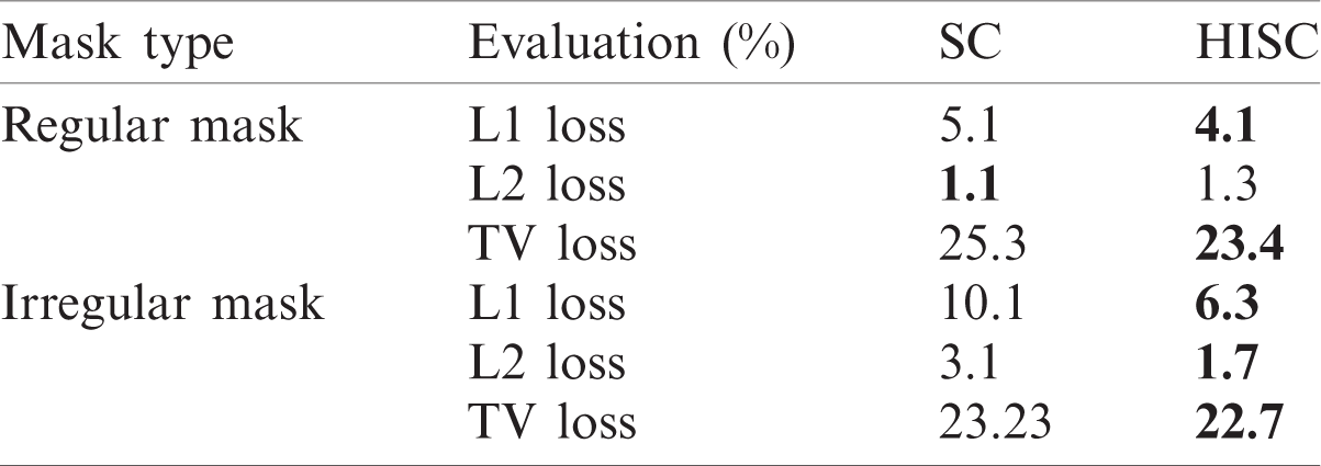
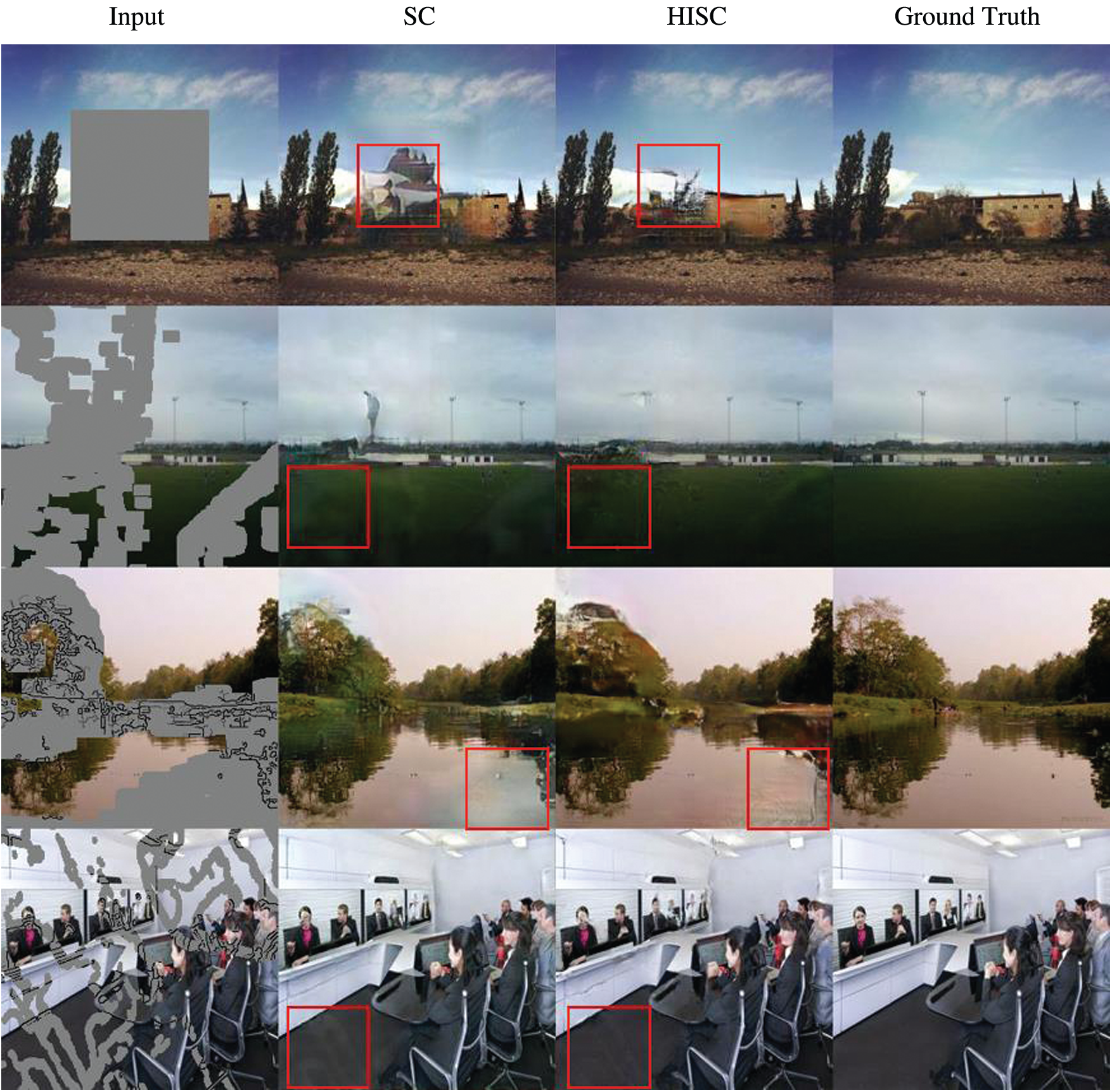
Figure 8: Inpainting results of HISC and SC for the Places2 test dataset. The top two images were generated without sketches, and the bottom two images were generated with sketches
Fig. 7 illustrates some of the inpainting results by the four models. Overall, our model outperformed the other models visually. For instance, Liu’s model produced pixels of different colors than the original color, especially in the background. DeepFill v2 produced some edges or regions in the first and fourth images that were not in the ground truth, although it exhibited reasonable restoration performance. However, the proposed model exhibited excellent restoration results for all images.
4.4 Skip Connection vs. Hadamard Identity Skip Connection
We compared the performance of UFC-net with HISC and UFC-net with SC to validate the effectiveness of HISC. In addition, we used the same conditions as in Sections 4.2 and 4.3 except for the sketch condition. We concatenated sketches during both training and testing with a 50% probability. Tab. 6 lists the evaluation results. The HISC outperformed the conventional SC in most cases, particularly for irregular masks. Fig. 8 illustrates the actual visual effects of HISC and SC in the UFC-net. The SC-based model generated an image in which the mask area and its surroundings were visually separated. In addition, the model adopting the SC technique often produced unintended shapes or colors, whereas HISC did so less often.
Table 7: Quantitative result comparison with 1, 2, 4, 8, and 16 latent fully connected layers
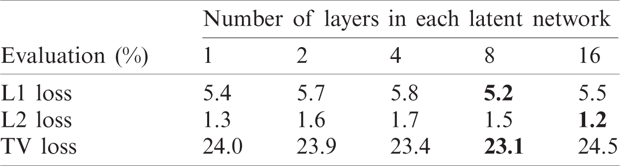
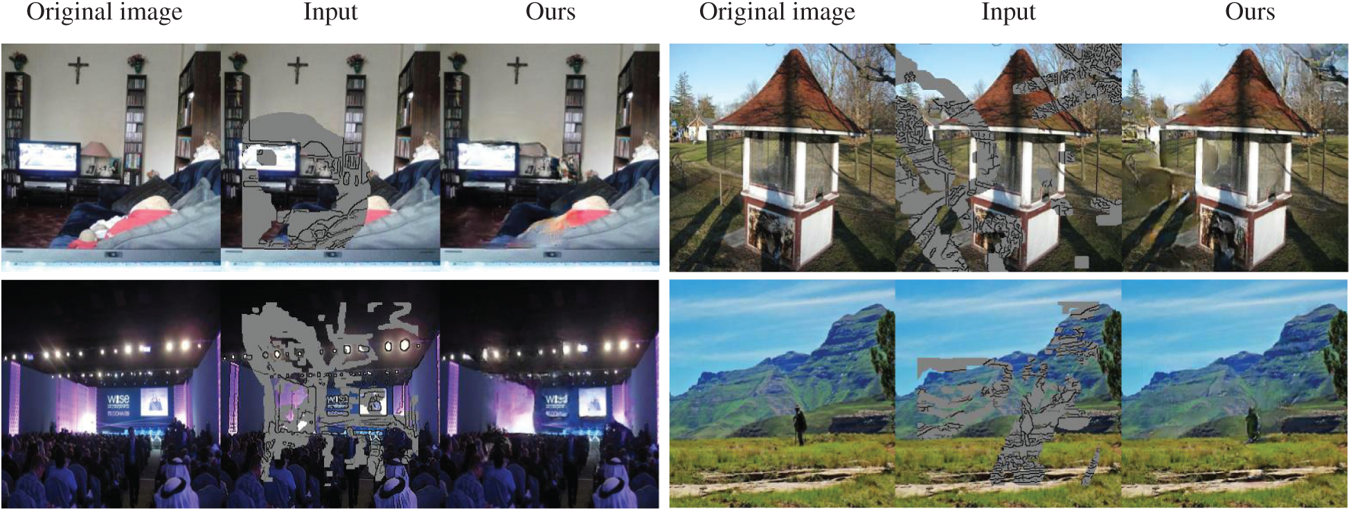
Figure 9: Example of using a sketch (black line) in the erased gray area of the original image
4.5 Effectiveness of the Latent Network and Sketch Input
In this experiment, we evaluated the accuracy of the model according to the number of latent network layers and summarized the results in Tab. 7. Eight FC layers achieved the best performance in L1 loss and TV loss. In contrast, 16 FC layers exhibited the lowest L2 loss. Fig. 9 illustrates the results of applying a sketch to our model. The image edges were determined along with the sketch, which indicates that the proposed model can perform sketch-based interactive image editing, like DeepFill v2 [15] and SC-FEGAN [19].
In this paper, we proposed an inpainting model by appending FC layers and HISC in the U-net. Our model not only extended the scope of spatial support but also transformed the input distribution to the output distribution smoothly using FC layers. In addition, HISC improved the reconstruction performance and reduced the computational cost compared to the original SC. Through extensive experiments using the Places2 dataset, we found that the proposed model outperformed the state-of-the-art inpainting models in terms of L1 loss and TV loss through diverse sample images. We also verified that HISC could achieve better performance than the original SC for regular and irregular masks. In the near future, we will consider other datasets for testing and improve the UFC-net to cover larger blank areas.
Funding Statement: This research was supported in part by NRF (National Research Foundation of Korea) Grant funded by the Korean Government (No. NRF-2020R1F1A1074885) and in part by the Brain Korea 21 FOUR Project in 2021.
Conflicts of Interest: The authors declare that they have no conflicts of interest to report regarding the present study.
1. A. Levin, A. Zomet, S. Peleg and Y. Weiss, “Seamless image stitching in the gradient domain,” in European Conf. on Computer Vision, Prague, Czech Republic, pp. 377–389, 2004. [Google Scholar]
2. E. Park, J. Yang, E. Yumer, D. Ceylan and A. C. Berg, “Transformation-grounded image generation network for novel 3d view synthesis,” in Proc. of the IEEE Conf. on Computer Vision and Pattern Recognition, Honolulu, HI, USA, pp. 3500–3509, 2017. [Google Scholar]
3. A. Criminisi, P. Pérez and K. Toyama, “Region filling and object removal by exemplar-based image inpainting,” IEEE Transactions on Image Processing, vol. 13, no. 9, pp. 1200–1212, 2004. [Google Scholar]
4. M. Bertalmio, G. Sapiro, V. Caselles and C. Ballester, “Image inpainting,” in Proc. of the 27th Annual Conf. on Computer Graphics and Interactive Techniques, New Orleans, LA, USA, pp. 417–424, 2000. [Google Scholar]
5. S. Esedoglu and J. Shen, “Digital inpainting based on the Mumford-Shah-Euler image model,” European Journal of Applied Mathematics, vol. 13, no. 4, pp. 353–370, 2001. [Google Scholar]
6. D. Liu, X. Sun, F. Wu, S. Li and Y.-Q. Zhang, “Image compression with edge-based inpainting,” IEEE Transactions on Circuits and Systems for Video Technology, vol. 17, no. 10, pp. 1273–1287, 2007. [Google Scholar]
7. C. Ballester, M. Bertalmio, V. Caselles, G. Sapiro and J. Verdera, “Filling-in by joint interpolation of vector fields and gray levels,” IEEE Transactions on Image Processing, vol. 10, no. 8, pp. 1200–1211, 2001. [Google Scholar]
8. S. Darabi, E. Shechtman, C. Barnes, D. B. Goldman and P. Sen, “Image melding: Combining inconsistent images using patch-based synthesis,” ACM Transactions on Graphics, vol. 31, no. 4, pp. 1–10, 2012. [Google Scholar]
9. J.-B. Huang, S. B. Kang, N. Ahuja and J. Kopf, “Image completion using planar structure guidance,” ACM Transactions on Graphics, vol. 33, no. 4, pp. 1–10, 2014. [Google Scholar]
10. D. Liu, X. Sun, F. Wu, S. Li and Y.-Q. Zhang, “Image compression with edge-based inpainting,” IEEE Transactions on Circuits and Systems for Video Technology, vol. 17, no. 10, pp. 1273–1287, 2007. [Google Scholar]
11. D. Pathak, P. Krahenbuhl, J. Donahue, T. Darrell and A. A. Efros, “Context encoders: Feature learning by inpainting,” in Proc. of the IEEE Conf. on Computer Vision and Pattern Recognition, Las Vegas, NV, USA, pp. 2536–2544, 2016. [Google Scholar]
12. S. Iizuka, E. Simo-Serra and H. Ishikawa, “Globally and locally consistent image completion,” ACM Transactions on Graphics, vol. 36, no. 4, pp. 1–14, 2017. [Google Scholar]
13. J. Yu, Z. Lin, J. Yang, X. Shen, X. Lu et al., “Generative image inpainting with contextual attention,” in Proc. of the IEEE Conf. on Computer Vision and Pattern Recognition, Salt Lake City, UT, USA, pp. 5505–5514, 2018. [Google Scholar]
14. G. Liu, F. A. Reda, K. J. Shih, T.-C. Wang, A. Tao et al., “Image inpainting for irregular holes using partial convolutions,” in Proc. of the European Conf. on Computer Vision, Munich, Germany, pp. 85–100, 2018. [Google Scholar]
15. J. Yu, Z. Lin, J. Yang, X. Shen, X. Lu et al., “Free-form image inpainting with gated convolution,” in Proc. of the IEEE/CVF Int. Conf. on Computer Vision, Seoul, Korea, pp. 4471–4480, 2019. [Google Scholar]
16. I. J. Goodfellow, J. Pouget-Abadie, M. Mirza, B. Xu, D. Warde-Farley et al., “Generative adversarial networks,” arXiv preprint arXiv:1406.2661, 2014. [Google Scholar]
17. B. Zhou, A. Lapedriza, A. Khosla, A. Oliva and A. Torralba, “Places: A 10 million image database for scene recognition,” IEEE Transactions on Pattern Analysis and Machine Intelligence, vol. 40, no. 6, pp. 1452–1464, 2017. [Google Scholar]
18. P. Teterwak, A. Sarna, D. Krishnan, A. Maschinot, D. Belanger et al., “Boundless: Generative adversarial networks for image extension,” in Proc. of the IEEE/CVF Int. Conf. on Computer Vision, Seoul, Korea, pp. 10521–10530, 2019. [Google Scholar]
19. Y. Jo and J. Park, “SC-FEGAN: Face editing generative adversarial network with user’s sketch and color,” in Proc. of the IEEE/CVF Int. Conf. on Computer Vision, Seoul, Korea, pp. 1745–1753, 2019. [Google Scholar]
20. O. Ronneberger, P. Fischer and T. Brox, “U-net: Convolutional networks for biomedical image segmentation,” in Int. Conf. on Medical Image Computing and Computer-Assisted Intervention, Munich, Germany, pp. 234–241, 2015. [Google Scholar]
21. G. Huang, Z. Liu, L. Van Der Maaten and K. Q. Weinberger, “Densely connected convolutional networks,” in Proc. of the IEEE Conf. on Computer Vision and Pattern Recognition, Honolulu, HI, USA, pp. 4700–4708, 2017. [Google Scholar]
22. K. He, X. Zhang, S. Ren and J. Sun, “Deep residual learning for image recognition,” in Proc. of the IEEE Conf. on Computer Vision and Pattern Recognition, Las Vegas, NV, USA, pp. 770–778, 2016. [Google Scholar]
23. K. Nazeri, E. Ng, T. Joseph, F. Qureshi and M. Ebrahimi, “Edgeconnect: Structure guided image inpainting using edge prediction,” in Proc. of the IEEE/CVF Int. Conf. on Computer Vision Workshops, Seoul, Korea, 2019. [Google Scholar]
24. J. Johnson, A. Alahi and L. Fei-Fei, “Perceptual losses for real-time style transfer and super-resolution,” in European Conf. on Computer Vision, Amsterdam, The Netherlands, pp. 694–711, 2016. [Google Scholar]
25. L. A. Gatys, A. S. Ecker and M. Bethge, “A neural algorithm of artistic style,” arXiv preprint arXiv:1508.06576, 2015. [Google Scholar]
26. Y. Ren, X. Yu, R. Zhang, T. H. Li, S. Liu et al., “Structureflow: Image inpainting via structure-aware appearance flow,” in Proc. of the IEEE/CVF Int. Conf. on Computer Vision, Seoul, Korea, pp. 181–190, 2019. [Google Scholar]
27. A. Krizhevsky, I. Sutskever and G. E. Hinton, “Imagenet classification with deep convolutional neural networks,” Communications of the ACM, vol. 60, no. 6, pp. 84–90, 2017. [Google Scholar]
28. M. D. Zeiler, D. Krishnan, G. W. Taylor and R. Fergus, “Deconvolutional networks,” in 2010 IEEE Computer Society Conf. on Computer Vision and Pattern Recognition, San Francisco, California, pp. 2528–2535, 2010. [Google Scholar]
29. F. Yu and V. Koltun, “Multi-scale context aggregation by dilated convolutions,” arXiv preprint arXiv:1511.07122, 2015. [Google Scholar]
30. Y. LeCun, B. Boser, J. S. Denker, D. Henderson, R. E. Howard et al., “Backpropagation applied to handwritten zip code recognition,” Neural Computation, vol. 1, no. 4, pp. 541–551, 1989. [Google Scholar]
31. A. Radford, L. Metz and S. Chintala, “Unsupervised representation learning with deep convolutional generative adversarial networks,” arXiv preprint arXiv:1511.06434, 2015. [Google Scholar]
32. X. Hong, P. Xiong, R. Ji and H. Fan, “Deep fusion network for image completion,” in Proc. of the 27th ACM Int. Conf. on Multimedia, New York, NY, United States, pp. 2033–2042, 2019. [Google Scholar]
33. Y. Ren, X. Yu, J. Chen, T. H. Li and G. Li, “Deep image spatial transformation for person image generation,” in Proc. of the IEEE/CVF Conf. on Computer Vision and Pattern Recognition, Seattle, United States, pp. 7690–7699, 2020. [Google Scholar]
34. T. Karras, S. Laine, M. Aittala, J. Hellsten, J. Lehtinen et al., “Analyzing and improving the image quality of stylegan,” in Proc. of the IEEE/CVF Conf. on Computer Vision and Pattern Recognition, Seattle, United States, pp. 8110–8119, 2020. [Google Scholar]
35. S. Ioffe and C. Szegedy, “Batch normalization: Accelerating deep network training by reducing internal covariate shift,” in Int. Conf. on Machine Learning, Lille, France, pp. 448–456, 2015. [Google Scholar]
36. P. Isola, J.-Y. Zhu, T. Zhou and A. A. Efros, “Image-to-image translation with conditional adversarial networks,” in Proc. of the IEEE Conf. on Computer Vision and Pattern Recognition, Honolulu, HI, USA, pp. 1125–1134, 2017. [Google Scholar]
37. T. Miyato, T. Kataoka, M. Koyama and Y. Yoshida, “Spectral normalization for generative adversarial networks,” arXiv preprint arXiv:1802.05957, 2018. [Google Scholar]
38. C.-I. Kim, M. Kim, S. Jung and E. Hwang, “Simplified fréchet distance for generative adversarial nets,” Sensors, vol. 20, no. 6, pp. 1548, 2020. [Google Scholar]
39. J. Canny, “A computational approach to edge detection,” IEEE Transactions on Pattern Analysis and Machine Intelligence, vol. 8, no. 6, pp. 679–698, 1986. [Google Scholar]
40. D. P. Kingma and J. Ba, “Adam: A method for stochastic optimization,” arXiv preprint arXiv:1412.6980, 2014. [Google Scholar]
41. M. Heusel, H. Ramsauer, T. Unterthiner, B. Nessler and S. Hochreiter, “Gans trained by a two time-scale update rule converge to a local nash equilibrium,” arXiv preprint arXiv:1706.08500, 2017. [Google Scholar]
 | This work is licensed under a Creative Commons Attribution 4.0 International License, which permits unrestricted use, distribution, and reproduction in any medium, provided the original work is properly cited. |