Computers, Materials & Continua DOI:10.32604/cmc.2021.017729
Article

Research on Forecasting Flowering Phase of Pear Tree Based on Neural Network

Zhenzhou Wang1, Yinuo Ma1, Pingping Yu1,*, Ning Cao2 and Heiner Dintera3

1School of Information Science and Engineering, Hebei University of Science and Technology, Shijiazhuang, 050000, China
2School of Internet of Things and Software Technology, Wuxi Vocational College of Science and Technology, Wuxi, 214028, China
3German-Russian Institute of Advanced Technologies, Karan, 420126, Russia
*Corresponding Author: Pingping Yu. Email: yppflx@aliyun.com
Received: 03 February 2021; Accepted: 08 March 2021

Abstract: Predicting the blooming season of ornamental plants is significant for guiding adjustments in production decisions and providing viewing periods and routes. The current strategies for observation of ornamental plant booming periods are mainly based on manpower and experience, which have problems such as inaccurate recognition time, time-consuming and energy sapping. Therefore, this paper proposes a neural network-based method for predicting the flowering phase of pear tree. Firstly, based on the meteorological observation data of Shijiazhuang Meteorological Station from 2000 to 2019, three principal components (the temperature factor, weather factor, and humidity factor) with high correlation coefficient with the flowering phase of pear tree are obtained by using the principal component analysis method. Then, the three components are used as input factors for the BP neural network. A BP neural network prediction model is constructed based on genetic algorithm optimization. The crossover operator and mutation operator in the adaptive genetic algorithm are improved. Finally, the meteorological sample data from 2013 to 2019 are used to test and verify the algorithm in this paper. The results demonstrate that, the model can solve the local optimization problem of the BP neural network model. The prediction results of the flowering phase of pear tree are evaluated in terms of relevance and prediction accuracy. Both are superior to the traditional effective accumulated temperature and the prediction results of the stepwise regression method. This method can provide more reliable forecast information for the blooming period, which can provide decision-making reference for improving the development of tourism industry.

Keywords: Pear flower; flowering phase; principal component analysis; BP neural network; prediction model

1  Introduction

Flowering period data of ornamental plants are important for the organization and development of flower-viewing tourism activities. These data can provide guidance for tourists to formulate flower viewing tourism plans, and provide reference for the planning of flower-viewing activities in scenic locations. Ornamental plants have a strong seasonal flowering period, short duration, and are easily affected by the external environment. The earlier the flowering period is monitored, the earlier best views and routs can be got. Traditional manual observation is time-consuming and laborious. It cannot effectively predict and release information in a timely manner.

There are many studies on the relationships among the plant flowering period and climate, climate change and prediction technology of flowering period. Gonsamo et al. [1] simulated the anomalous changes in the initial flowering of 19 Canadian plants since 1948. Morin et al. [2] predicted the changes in the initial leaf development of 22 woody plants in North America in the next 100 years. Zhong et al. [3] established a temperature-based temporal and spatial prediction model for the flowering period of Chinese ornamental plants. Liu et al. [4] used wavelet analysis, correlation analysis and other methods to assess the impacts of climate change on flowering phase of peach blossom. Aono [5] investigated the phenological data of cherry blossoms in Edo since the 17th century and their application in March temperature estimation. Ahn et al. [6] conducted a seasonal forecast of surface temperatures and the first flowering period in Korea. At present, the effective accumulated temperature rule is mainly used to predict the flowering phase, that is, the effective accumulated temperature for a certain period of time after the plant’s flowering threshold temperature is met. Dong et al. [7] analyzed the relationships between the flowering phase of peach trees and temperature elements by using the phenological observation data of peach trees in the blooming period and the daily average temperature observation data of the climate station in the Hekou area of Dandong City. The active accumulated temperature, effective accumulated temperature, and sliding accumulated temperature were used to predict the blooming periods of peach trees in the Dandong area. Through analysis, Yao et al. [8] found that the temporal accumulated temperature phase had a small correlation with the variation coefficient of daily accumulated temperature, but had a large correlation with the absolute value of the correlation coefficient of daily ordinal number at flowering stage. These results indicate that temporal accumulated temperature can better reveal the internal relationship between accumulated temperature and crop growth on a smaller time scale. Judging the flowering phase of plants by accumulated temperature is simple to perform and has a certain biological basis. However, because this method disregards the influences of meteorological factors such as sunlight and precipitation on the flowering period, the accuracy of the predicted flowering period is low.

With the development of computational science, neural networks have been widely investigated and applied in various fields of science and engineering, and relatively satisfactory prediction results have been achieved. Long et al. [9] employed a 3-layer BP neural network to establish a fog forecast model. Based on the air pollutant data of Delhi, India, from 2014 to 2016. Ganesh et al. [10] established an artificial neural network prediction model that is based on the conjugate gradient descent method to predict the air quality index in a specific area. Zhang et al. [11] proposed a BP neural network earthquake damage prediction model that is based on the LM algorithm, which can realize that only part of the key data of a single building needs to be extracted. He et al. [12] established a BP neural network soil temperature prediction model that is optimized by a genetic algorithm to accurately predict the soil temperature in winter orchards. Aiming at the problem of single sources of forecast data and low accuracy in current atmospheric visibility forecasting algorithms. Wang et al. [13] constructed a BP neural network model optimized based on a genetic algorithm. Pooya et al. [14] employed artificial neural networks (ANNs), genetic algorithms and artificial neural network integration (GAINN) to predict the efficiency of fiber filters. Sun et al. [15] established a rape blossom forecast model based on the BP neural network and explored the application of the BP neural network in the field of flowering forecast. Neural network technology provides a new way to simulate and predict flowering.

Aimed at forecasting the flowering phase of ornamental plants, existing research focuses on cherry blossoms, while there are few simulations of the flowering phase of other ornamental plants. This paper propose a prediction method based on neural network for flowering phase of pear trees. Through principal component analysis, three principal components with higher correlation coefficient with the flowering phase of pear trees were obtained as input factors of the neural network. The problem of low accuracy of the forecasted flowering period is improved. This paper is organized as follows: In the second section, the sources of pear phenological data were introduced, and three principal components were obtained by using principal component analysis. In the third section, a BP neural network model is established based on genetic algorithm optimization, and the model parameters are instantiated. In the fourth section, the model is trained and tested, and compared with the traditional effective accumulated temperature method. The fifth section uses the trained model to forecast the flowering stage of pear trees in 2020. In the last, a conclusion is provided.

2  Data Sources and Research Methods

2.1 Flowering Data of Pear Trees

The phenological data of pear flowers were obtained from the observation data of pear trees planting area provided by Shijiazhuang Meteorological Bureau from 2009 to 2020. The observation basis and standards are the “China Phenological Observation Network” observation standards and the China Meteorological Administration “Agricultural Meteorological Observation Specifications.” The initial flowering period of a plant is defined as the data when the first fully open flower begins to appear on the observation plant. The full bloom period is defined as the data when more than half of the flower buds on the observation plant unfold and show the petals [16].

The flowering day ordinal number is the conversion of the observation date into a diurnal sequence. January 1 is taken as the beginning data of the flowering diurnal sequence, and the diurnal number is 1, and so on, such as February 5, the diurnal number is 36 [17].

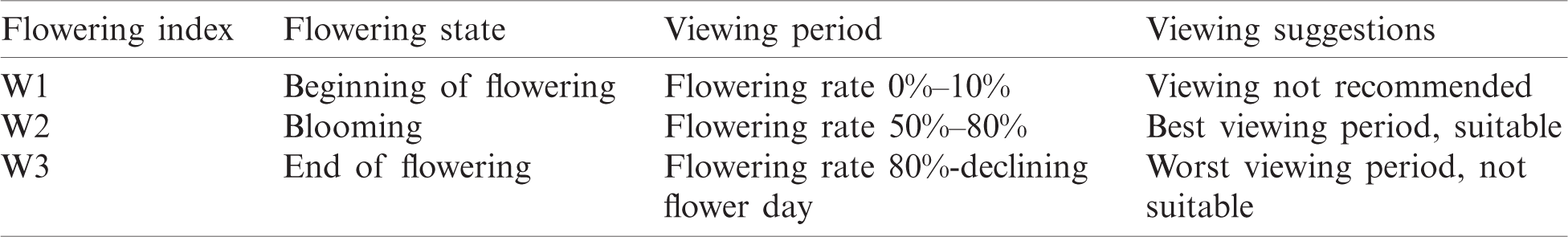
By analyzing the location observation phenological data and parallel observation meteorological data of the pear trees planting area from 2009 to 2020, it is calculated that the average initial flowering time of pear trees is April 3; the average blooming period is April 10; and the average end of flowering is April 20. The earliest flowering date is March 20, and the latest data is April 16. The flowering phase begins as early as March 28 and as late as April 24. The earliest date of the end of flowering is April 8, and the latest date is May 4. The flowering phase of pear trees lasts for approximately 20 days on average from the beginning to the end of flowering. According to years of observation and analysis, pear blossoms will enter a suitable viewing period after 2–3 days of initial flowering [18], as shown in Tab. 1.

Table 1: Design index of pear blossom index

2.2 Meteorological Factors Determining by Principal Component Analysis Method

2.2.1 Selection of Meteorological Factors

Meteorological factors, including temperature, precipitation, sunshine, etc., impose obvious constraints on the growth of pear trees. However, the restrictive effects of different meteorological factors are divided into strong and weak factors that are relatively independent.

This paper selects the daily maximum temperature, daily minimum temperature, daily average temperature, daily precipitation, daily sunshine duration, daily average ground temperature and daily average relative humidity from 2000 to 2019 at Shijiazhuang City Meteorological Station. These data have been strictly controlled by artificial quality. The average values of each meteorological element in winter from 2001 to 2019 are obtained by calculation.

2.2.2 Principal Component Analysis Method

Principal Component Analysis (PCA) aims to analyze the characteristics of the covariance matrix to reduce the dimensionality of the data while maintaining the largest contribution to the variance of the data set [19]. By dimensionality reduction, the original index is transformed into one or several comprehensive indexes: namely, principal components. The principal components are not correlated. The steps of the principal component analysis to analyze the meteorological factors related to pear flower blooming are described as follows:

Step 1: Select the meteorological factors that are related to the flowering period of pear blossoms, and perform z-score normalization (zero-mean normalization) on the original data. The formula is expressed as follows:

xij*=(xij-x¯j)/sj(1)

In the formula, x*ij is the standardized meteorological factor, xij is the original data of each meteorological factor, and x¯j and sj are the mean and standard deviation, respectively, of each meteorological factor.

Step 2: Calculate the correlation coefficient matrix R of the standardized meteorological factor data:

Rij=∑k=1n(|xki-x¯i||xkj-x¯j|)∑k=1n(xki-x¯i)2∑k=1n(xkj-x¯j)2(2)

In the formula, Rij is the correlation coefficient between the i-th standardized index and the j-th standardized index.

Step 3: According to the meteorological factor correlation coefficient matrix R, find the eigenvalue, the contribution rate of the principal component and the contribution rate of the cumulative variance. Determine the number of principal components, and solve the characteristic equation:

|λE-R|=0(3)

Find the eigenvalue λi (i=1,2,…,p), where p is the number of main components. The eigenvalue is the variance between the principal components, which reflects the influence of each principal component. The sharing rate of the principal component Wi is:

Wi=λj/∑j=1pλj(4)

Cumulative contribution rate:

∑j=1mλj/∑j=1pλj(5)

According to the principle of selecting the number of principal components, eigenvalues greater than 1 and cumulative contribution rates greater than 90% are selected.

2.2.3 Results of Principal Component Analysis Method

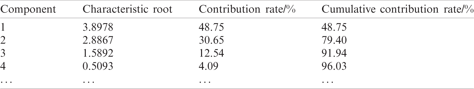
The meteorological observation data of meteorological stations from 2000 to 2019 were used, and the eigenvalues of the correlation matrix and the contribution rate of each principal component were obtained. The results are shown in Tab. 2. M principal components with characteristic roots greater than 1 and cumulative contribution rates greater than 90% are selected. From Tab. 2, the characteristic roots of the first three are greater than 1, and the cumulative contribution rate reaches 91.94%. The three principal components can reflect most of the information of the original meteorological indicators. This process can reduce the complexity of the original data and achieve the purpose of dimensionality reduction.

Table 2: 2000–2019 Shijiazhuang weather station sample correlation coefficient matrix eigenvalues

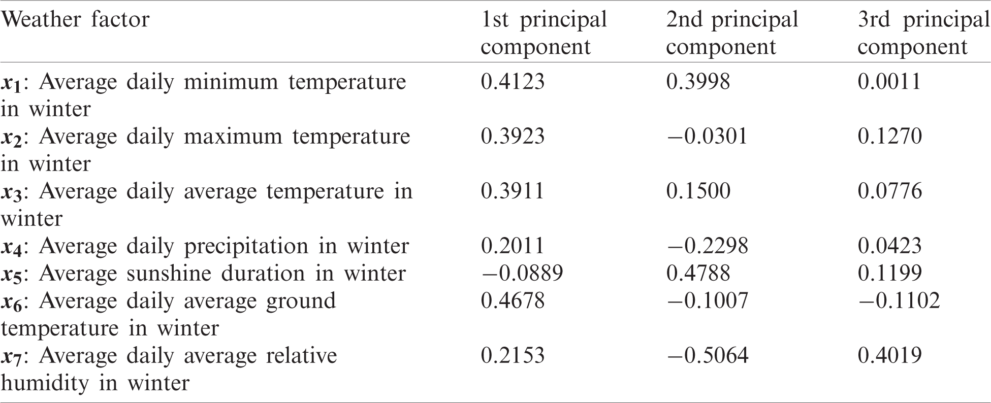
The eigenvectors of the three principal component factors are listed in Tab. 3. Tab. 3 shows that for the eigenvector of the first principal component, the factors with larger and positive eigenvalues are the average daily minimum temperature in winter, average daily maximum temperature in winter, average daily average temperature in winter, and average daily average ground temperature in winter. The flowering period is closely related to temperature, so the first principal component can be referred to as the temperature factor. For the eigenvector of the second principal component, the factor with a larger and positive eigenvalue is the average sunshine duration in winter, the larger and negative factor is the average daily precipitation in winter and the average daily average low temperature in winter. Therefore, the flowering period is obviously positively correlated with sunshine duration and negatively correlated with precipitation and relative humidity. The second principal component is referred to as the weather factor. Among the eigenvectors of the third principal component, the factor with a large and positive eigenvalue is the average daily average relative humidity in winter, which can be referred to as the humidity factor.

Table 3: Principal component feature vector of meteorological data from Shijiazhuang Meteorological Station 2000–2019

According to the characteristic vector of the principal components (Tab. 3), the linear equations between the three principal components and the meteorological factors can be obtained:

F1=0.4123x1+0.3923x2+0.3911x3+0.2011x4-0.0889x5+0.4678x6+0.2153x7 (6)

F2=0.3998x1-0.0301x2+0.1500x3-0.2298x4+0.4788x5-0.1007x6-0.5064x7 (7)

F3=0.0011x1+0.1270x2+0.0776x3+0.0423x4+0.1199x5-0.1102x6+0.4019x7 (8)

In addition, studies have pointed out that environmental parameters such as soil temperature, cold demand and hourly accumulated temperature, as well as management measures such as tree age, fertilization and irrigation, are also related to the flowering phase of trees. This article forecasts the overall flowering period in the region from the perspective of weather forecasting services, instead of a single fruit tree or orchard. Taking into account the availability of data, these parameters are not involved.

3  BP Neural Network Prediction Model Based on An Improved Genetic Algorithm

The research and application of neural networks in various fields of science and engineering are extensive, and relatively satisfactory prediction results have been achieved. The BP neural network, which is the most commonly employed from of artificial neural network [19], has a nonlinear mapping ability and excellent fault tolerance and can be applied to the flowering period prediction model of this article. The learning process of the BP neural network is actually a process of training the network with training samples [20]. Aimed at problems such as difficulty in forecasting the flowering period of ornamental plants and inaccurate prediction of long-term data, this paper uses an improved genetic algorithm to iteratively identify the structure and designs a BP neural network prediction model that is based on genetic algorithm optimization for flowering prediction.

3.1 Neural Network Structure

The BP neural network is generally composed of an input layer, a hidden layer and an output layer. And a large number of neurons are connected to each other as network nodes [21]. Considering a 3-layer neural network as an example, set the input layer to xi, the hidden layer to yh, the output layer to ol, and the expected value of output to tl. The structure diagram is shown in Fig. 1.

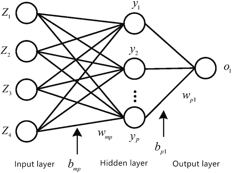
Figure 1: BP neural network structure diagram

The error function between the output and the expected value is:

∂E∂vlh=-δloh (9)

δl=(tl-zl)⋅f′(∑ vlhoh-θl) (10)

where θl is the threshold and f′ is the inverse function of the transfer function.

∂E∂whi=-δl′xi (11)

δh′=f′(∑ whixi-θh)⋅∑ δlvlh (12)

where θh is the threshold, and the weight in the k + 1 iteration is

vlh(k+1)=vlh(k)+Δvlh (13)

whi(k+1)=whi(k)+Δwhi (14)

Because δvlh=-η⋅∂E/∂vlh=ηδlyh, δwhi=-η′⋅∂E/∂whi=η′δh′xi, the threshold of the output layer and the change in the threshold of the hidden layer can be expressed as

θl(k+1)=θl(k)+ηδl (15)

θh(k+1)=θh(k)+η′δh′ (16)

where η and η′ are the learning rates.

3.2 Improved Adaptive Crossover Operator and Mutation Operator

Traditional genetic algorithms use fixed crossover probability and mutation probability [22]. The crossover probability is generally selected between 0.3 and 0.7, and the mutation probability is generally selected between 0.1 and 0.3 [23]. However, it is difficult to optimize the crossover and mutation probability. If a larger crossover probability is selected, new individuals will be generated too quickly, and individuals with high fitness values are easily destroyed, which may cause the algorithm to evolve into a random search algorithm. If a smaller crossover probability is selected, new individuals will be generated. If the speed is too slow, the algorithm can easily fall into the local optimum. If a larger mutation probability is selected, although the diversity of the population can be maintained, the advanced mode of population inheritance will be destroyed. If a small mutation probability is selected, the diversity of the population will gradually decrease, which leads to the rapid loss of outstanding individuals and failure to achieve the desired result [24]. Due to the various shortcomings of traditional genetic algorithms, many scholars have continuously improved and proposed many improved algorithms, such as the adaptive genetic algorithm (AGA). The formula of the AGA is presented as

Pc={k1(fmax-f′)fmax-favg,f′≥favgk2,f′<favg (17)

Pm={k3(fmax-f′)fmax-favg,f′≥favgk4,f′<favg (18)

where f′ is the larger fitness value of the two individuals to be crossed; fmax is the maximum fitness in the population; favg is the average fitness of the population; f represents the fitness of the variant individual; and k1 − k4 are adaptive control parameters. However, AGA evolves slowly in the initial stage and is prone to stagnation. Excellent individuals are in a static state: that is, no crossover and mutation operations occur. At this time, individuals with high fitness values in the population are likely to converge locally and fail to reach the global optimum. The genetic algorithm can easily evolve in the direction of local convergence. Therefore, this article improves adaptive crossover probability and mutation probability as

Pc={pcmin-(pcmax-pcmin)(f′-favg)fmax-favg,f′≥favgpcmax,f′<favg (19)

Pm={pmmin-(pmmax-pmmin)(fmax-f)fmax-favg,f′≥favgpmmax,f′<favg (20)

where pcmin and pcmax represent the lower limit and upper limit, respectively, of the crossover rate; pmmin and pmmax represent the lower limit and upper limit, respectively, of the mutation rate. The individual’s crossover rate and mutation rate are still linearly transformed between the average fitness and the maximum fitness according to the fitness of the individual.

3.3 Establishment of the BP Neural Network Model Based on Genetic Algorithm Optimization

To improve the stability of the BP algorithm and solve the problem of local optimal solutions, this paper constructs a BP neural network model that is based on genetic algorithm optimization [25]. The genetic algorithm does not rely on gradient information and uses its global search advantages to optimize the BP neural network to obtain the best solution to the problem [26]. The genetic algorithm uses binary coding to assign a real number string to each individual of the population, and the population individual represents all the weights and thresholds of the BP neural network layer. According to the designed fitness value, the coded individual is employed to train the BP neural network, and then by the processes of selection, crossover, mutation, etc., the structure is iteratively identified by the improved genetic algorithm. Assume that there are a total of N fuzzy rules and the improved genetic algorithm is utilized for identification. In the identification process, the fitness of all individuals in the population P(t) is F1 = 1/J. The specific process is described as follows:

(1) Initialize the population P(0). Refer to the range of the data vector to perform coding operations to generate NC individuals as the initial population P(t) and set the maximum number of iterations T. The initial chromosomes are composed of regular codes that are generated by the BP algorithm.

(2) Calculate the fitness function. The fitness function F, which is also known as the evaluation function, can realize the measurement of the pros and cons of individuals in the group. The fitness function can be expressed by the sum of the absolute value of the error between the predicted output of the BP neural network and the actual output. The calculation formula is

F(x)=k(∑i=1nabs(yi-oi))(21)

(3) The selection operation is performed after completing the evaluation of the fitness function. The commonly employed selection methods of genetic algorithms include the fitness ratio method, partial selection method and roulette selection method. This article chooses the roulette selection method. The probability of an individual that is selected in this method is proportional to the fitness value that is calculated in Step (2). Assume that the fitness of individual i is fi; then

pi=fi/∑j=1nfi(22)

where n is the size of the group and pi is the probability that individual i will be selected.

(4) Crossover operation. Crossover operation refers to the operation of partially reorganizing the structure of the two selected first-generation individuals according to the principle of cross-exchange of biological chromosomes to form a new individual, and the crossover operation acts on the selected group. The crossover probability is Pc.

(5) In the mutation operation, the mutation operator judges the mutation probability of the individual in the group and then randomly selects the mutation position of the mutated individual to obtain the result of the mutation. The mutation operation is applied to the selected population. The mutation probability is Pm.

(6) After the population P(t) completes Steps (3)–(5), the next generation population P(t+1) is obtained.

(7) If the termination condition is met, proceed to the decoding operation; otherwise, return to Step (3).

The overall design process is shown in Fig. 2:

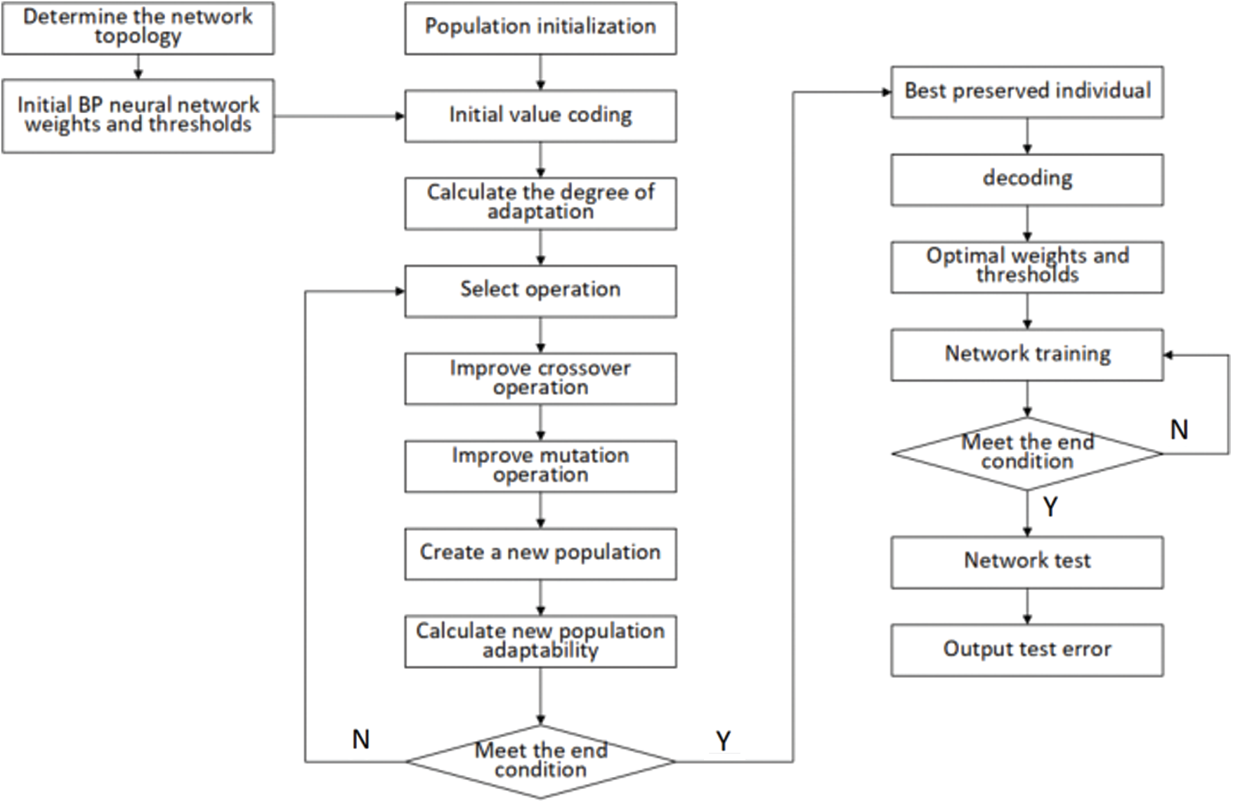
Figure 2: Improved genetic algorithm BP neural network process

3.4 Model Parameter Setting

This study selects a 3-layer BP neural network and uses principal component analysis to obtain three principal component factors that affect the flowering phase of pear trees as the input layer of the BP neural network. Coupled with the input layer threshold, the model has 4 input vectors. The daily ordinal number of the full-blossom period of pear trees (best viewing period) is utilized as the output vector of the output layer, and thus the number of nodes in the output layer is 1, and the output vector is 1. The determination of the number of neurons in the hidden layer is related to the actual problem that needs to be solved, and the optimal number of neurons is generally determined by a formula.

m=n+q+α(23)

where n is the number of neurons in the input layer, q is the number of neurons in the output layer, α is an integer in [1, 10], and m is the number of neurons in the hidden layer. The determination of the number of hidden layers has an important role in the accuracy of the prediction model [26]. In the case of the same sample test, this paper compares the training errors using different hidden layer numbers and obtains the results in Tab. 4 via 6 trials. It can be seen from the test results that when the number of hidden layers is 6, the training error is 0.1868, and the best training result is obtained.

Table 4: Network training error of different hidden layer nodes

The relevant parameters of the genetic algorithm are listed as follows: the number of iterations is 10; the randomly generated population size is 100; the crossover rate Pc = 0.3, and the mutation rate Pm = 0.1.

4  Result Analysis

4.1 Model Training and Test Results

This article uses the MATLAB R2014a neural network development toolbox and Sheffield genetic algorithm toolbox for training. In the process of training the determined network structure, to prevent “transition training,” the network adopts the following convergence rules: if the samples with an absolute error of less than 2 reach 85% of the total samples, the training is stopped. Otherwise, the maximum number of training iterations (10,000 iterations) is specified, and the samples are used to verify the network when the training meets the requirements.

In this paper, the flowering phenology data of pear trees from 2000 to 2012 in the pear planting area of Shijiazhuang are employed as the training input samples of the BP neural network. A trial report is conducted using the 2013–2019 sample. When using the three main component factors as the network input, the comprehensive situation of the meteorological factors is considered, the main factor is enlarged and the secondary factor is weakened. Network training and testing were carried out according to the forecast model, and the training effect map (Fig. 3) and prediction effect map (Fig. 4) were drawn via training.

Comparing Figs. 3 and 4, it can be seen that the average error of the BP neural network training, which is based on genetic algorithm optimization with 3 principal component factors as input, is 1.5 days, and the training effect is reasonable. This finding shows that the forecast model has practical application value.

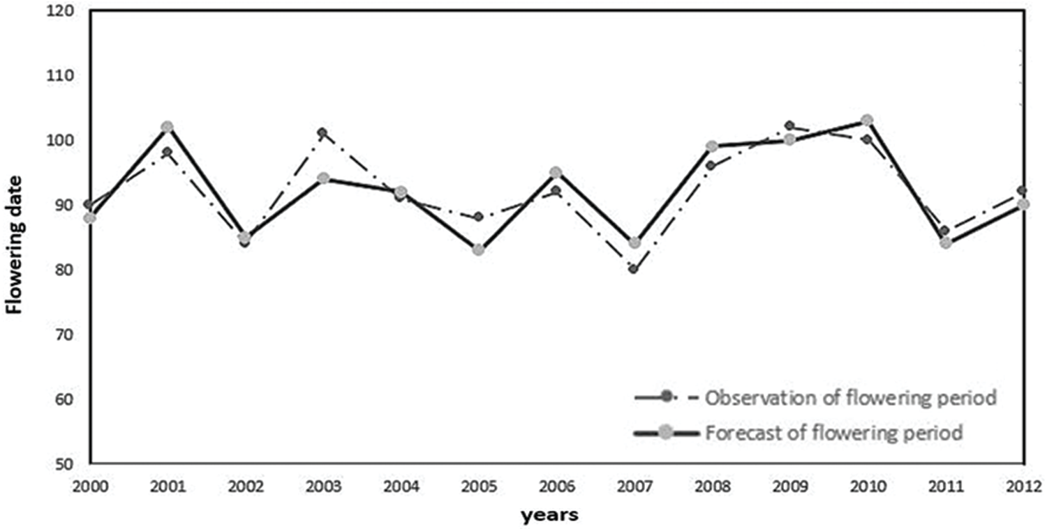
Figure 3: Training effect diagram

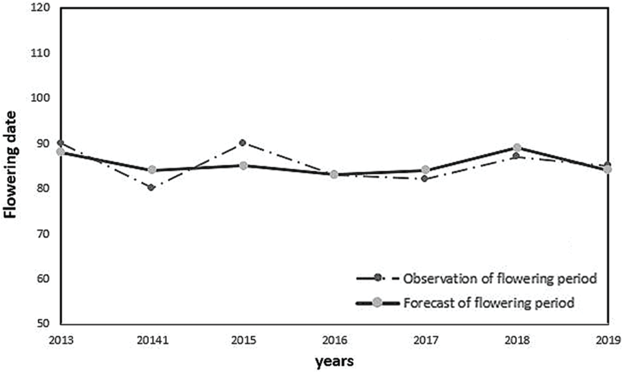
Figure 4: Forecast effect diagram

4.2 Analysis of Results of Different Forecasting Models

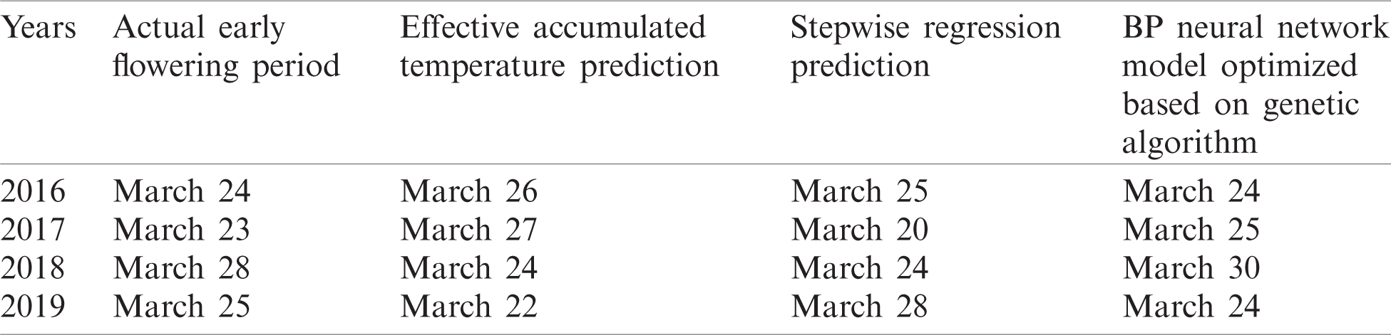
Using the data samples of the flowering phase of pear trees from 2016 to 2019, the improved BP neural network method proposed in this article, the traditional effective accumulated temperature law method and stepwise regression method are verified. The verification results of the three methods are shown in Tab. 5. From the table, we can see that the error of the flowering period forecast using the BP neural network model, which is optimized based on the genetic algorithm, is 1 day. The result for the effective accumulated temperature prediction method is 3.25 days, and that of the stepwise regression prediction method is 2.75 days. The flowering date predicted by this paper is closer to the actual flowering date. The meteorological factors filtered by the principal component analysis are used as model inputs, and the modeling method based on the BP neural network optimized by the genetic algorithm improves the accuracy of flowering forecasting.

Table 5: Forecast results of different forecast models

4.3 Accuracy of Flowering Fitting

To intuitively compare the applicability and accuracy of the method in this paper for the prediction of the flowering phase of pear trees in Shijiazhuang, a combination of internal inspection and cross-checking is employed. First, internal inspection is carried out. The parameters fitted from 2000 to 2019 are used to simulate the phenological sequence of the flowering phase of pear trees. The observed sequence of the flowering phase of pear trees is compared with the simulated sequence, and the variance (R2), significance and root mean squared error (RMSE) are calculated. Second, cross-check (also referred to as external check) is conducted. Cross-check adopts the method of elimination one by one, that is, after eliminating the observed value of flowering phase of pear trees in a certain year, the data of other years are used to fit parameters to simulate the phenological period of the eliminated year (full blooming period). After each year’s observations are separately eliminated, the series for cross-checking can be obtained. Additionally, we compare and analyze this sequence with respect to the phenological observation sequence.

R2=1-∑i=1n(di(x)-diobs)2∑i=1n(di(x)2-diobs)2 (24)

RMSE=∑i=1n[di(x)-diobs]2n (25)

where di(x) is the original date sequence of the flowering phase of pear trees; di(x)2 is the square of the original date sequence of the flowering phase of pear trees; diobs is the date sequence of the flowering phase of pear trees simulated by the model; and n is the number of test samples.

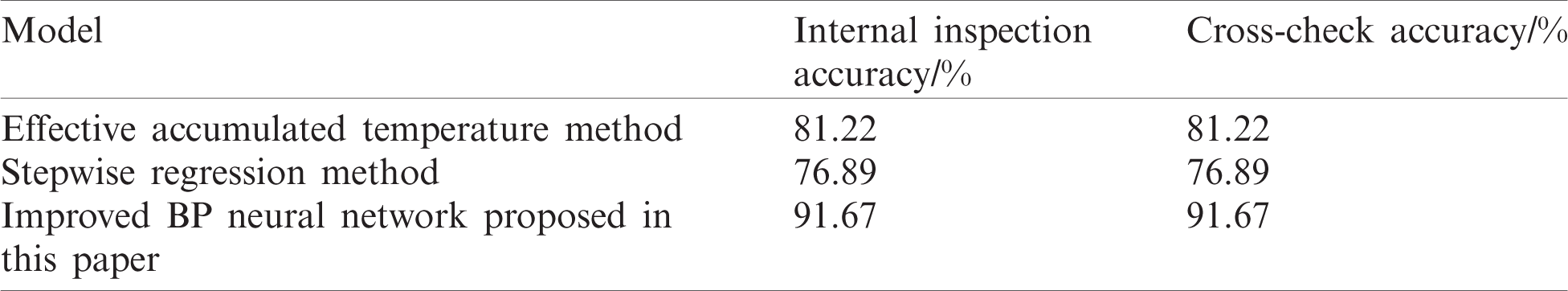
We compare and analyze the actual observation sequence of the flowering phase of pear trees with the simulated sequence of a certain year. If the difference between the two sequences is less than 3 days, the prediction is considered accurate and recorded as “1”; otherwise, the prediction is considered wrong and recorded as “0”. The accuracy of the forecast is the percentage of the number of accurate forecasts in the total number of years. It can be seen from Tab. 6 that the prediction accuracy of the algorithm in this paper is higher.

Table 6: The prediction accuracy of the three algorithms

5  Trial Report of the Flowering Phase of Pear Trees

After the training is completed, the topology of the neural network is readjusted. The number of nodes in the input layer includes the number of weather factors, the number of days in the initial flowering period and the accumulated temperature since the initial flowering period. The number of nodes in the output layer is the number of forecasted objects (1, use 1/0 to indicate whether flowering occurs the next day).

Accumulated temperature refers to the daily average temperature that is accumulated in the corresponding period of time when a plant completes a certain period or all-growth period. Accumulated temperature is an important indicator to measure the requirements of crop growth for thermal conditions and to evaluate thermal resources. According to the statistics of the accumulated temperature from January 1 to the full flowering period of pear blossom in Shijiazhuang City, the daily average temperature is greater than or equal to the threshold temperature of pear trees (any value in the range of 0.1–20.0∘C). The relationship between the accumulated temperature and the flowering period is analyzed to determine the most stable accumulated temperature threshold of 6.9∘C in this experiment.

A sample of a certain year is selected to form a calculation sample of the model in this paper within 10 days before and after flowering. The forecast value is 1 from the day before the flowering period, which indicates that the next day has entered the flowering period, and the number of days before that is set to 0. For example, the initial of flowering period of a certain year is March 20, the starting data of the sample is March 10–29, the forecast result before March 19 is 0, and the forecast result from March 19 is 1. The flowchart is shown in Fig. 5.

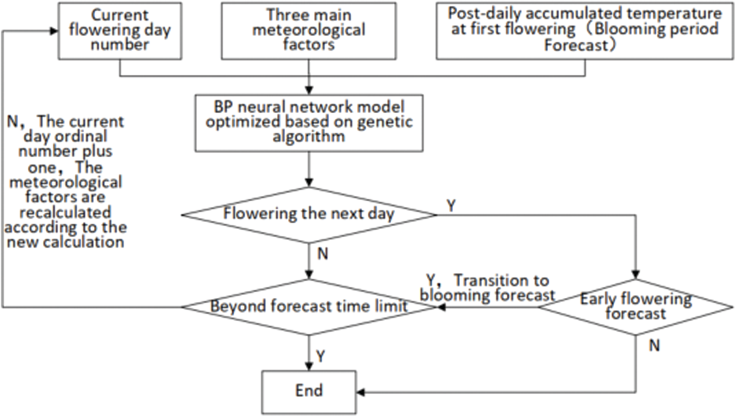
Figure 5: Forecast flow chart

Using the flowering period forecast model in this paper, the flowering phase of pear trees in 2020 in the Shijiazhuang area is forecasted. The forecast will be carried out every day beginning on March 1st. The maximum forecast time limit is 10 days, that is, the cycle in Fig. 5 is iterated 10 times. If the forecast result is 0, it is considered that no flowering will occur within 10 days. If 1 appears on the first time in the cycle, the next day is considered to be the flowering period. After the initial flowering data is forecasted, the blooming day forecast will continue. The first cycle means that March 25 predicts whether blooming will occur on March 26. If the result is 0, the second cycle begins to predict whether blooming will occur on March 27. If the result is 1 for three cycles, then the forecast result indicates that blooming will occur on March 28 (error of 0 day). If the results of 1 appears after 8 cycles, then the forecast result indicates that blooming will occur on April 4 (with an error of 1 day). In terms of service, the model provides a reasonable reference for the public to schedule their visits and has achieved excellent social benefits.

6  Conclusion

This paper selects the pear trees planting area in Shijiazhuang as the target area for prediction. Three principal component factors that affect the flowering period of pear are obtained through principal component analysis, namely, the temperature factor, weather factor and humidity factor. The BP neural network optimized based on a genetic algorithm is applied to the forecasting of the pear flowering period, and the crossover operator and mutation operator in the adaptive genetic algorithm are improved. The experimental results show that the error of the flowering period forecast using the forecast model in this paper is 1 day, the value of the effective accumulated temperature forecast method is 3.25 days, and that of the stepwise regression forecast method is 2.75 days. It can be seen that the algorithm proposed in this paper achieves better results than the traditional methods in predicting the flowering period, and also verifies the correlation between the flowering data and meteorological factors. The algorithm presented in this paper can provide more reliable forecast information of the flowering phase and provide reasonable reference for the public’s travel arrangement.

Funding Statement: This research was funded by the Science and Technology Support Plan Project of Hebei Province (Grant Number 19273703D) and the Science and Technology Research Project of Hebei Province (Grant Number ZD2020318).

Conflicts of Interest: The authors declare that they have no conflicts of interest to report regarding the present study.

This work is licensed under a Creative Commons Attribution 4.0 International License, which permits unrestricted use, distribution, and reproduction in any medium, provided the original work is properly cited.