DOI:10.32604/cmc.2021.016341
| Computers, Materials & Continua DOI:10.32604/cmc.2021.016341 | |
| Article |
Robust Magnification Independent Colon Biopsy Grading System over Multiple Data Sources
1Department of Computer Science and Engineering, Amrita School of Engineering, Amrita Vishwa Vidyapeetham, Bengaluru, India
2Department of Pathology, MVR Cancer Center and Research Institute, Poolacode, Kerala, India
3College of Computer and Information Sciences, King Saud University, Saudi Arabia
4Computer Engineering Department, College of Computer and Information Sciences, King Saud University, Saudi Arabia
*Corresponding Author: Tripty Singh. Email: tripty_singh@blr.amrita.edu
Received: 30 December 2020; Accepted: 13 March 2021
Abstract: Automated grading of colon biopsy images across all magnifications is challenging because of tailored segmentation and dependent features on each magnification. This work presents a novel approach of robust magnification-independent colon cancer grading framework to distinguish colon biopsy images into four classes: normal, well, moderate, and poor. The contribution of this research is to develop a magnification invariant hybrid feature set comprising cartoon feature, Gabor wavelet, wavelet moments, HSV histogram, color auto-correlogram, color moments, and morphological features that can be used to characterize different grades. Besides, the classifier is modeled as a multiclass structure with six binary class Bayesian optimized random forest (BO-RF) classifiers. This study uses four datasets (two collected from Indian hospitals—Ishita Pathology Center (IPC) of 4X, 10X, and 40X and Aster Medcity (AMC) of 10X, 20X, and 40X—two benchmark datasets—gland segmentation (GlaS) of 20X and IMEDIATREAT of 10X) comprising multiple microscope magnifications. Experimental results demonstrate that the proposed method outperforms the other methods used for colon cancer grading in terms of accuracy (97.25%-IPC, 94.40%-AMC, 97.58%-GlaS, 99.16%-Imediatreat), sensitivity (0.9725-IPC, 0.9440-AMC, 0.9807-GlaS, 0.9923-Imediatreat), specificity (0.9908-IPC, 0.9813-AMC, 0.9907-GlaS, 0.9971-Imediatreat) and F-score (0.9725-IPC, 0.9441-AMC, 0.9780-GlaS, 0.9923-Imediatreat). The generalizability of the model to any magnified input image is validated by training in one dataset and testing in another dataset, highlighting strong concordance in multiclass classification and evidencing its effective use in the first level of automatic biopsy grading and second opinion.
Keywords: Colon cancer; grading; texture features; color features; morphological features; feature extraction; Bayesian optimized random forest classifier
Colorectal cancer is one of the world’s most common cancers and is the second leading cause of cancer death [1]. In 2018, it ranked the third and second-most-common cancer for both genders’ incidence and mortality globally, constituting respectively 6.1% and 5.8% of the number of new cases and deaths, among all cancers combined worldwide [2]. The general cancer diagnosis process is tedious and reliant on experts using microscopic analysis of biopsy samples. An essential task for pathologists who analyze colon specimens across various magnifications in a microscope (4X, 5X, 10X, 20X, and 40X) is to distinguish invasive cancer and, to provide an accurate diagnosis and grading critical for the treatment plan. The subjective character of grading evaluation and the different patterns that many tumors exhibit render it difficult to achieve consistency between pathologists. This method requires a substantial amount of time to provide results in both inter-and intra-observer variations [3,4]. Owing to the visual discrepancy among observations, analyzing the sample under a microscope at various magnifications is crucial for an accurate diagnosis. The golden standard for diagnosis is an analysis by pathologists with subspecific expertise and specialty in gastrointestinal malignancy. However, second opinions are slow to come, work-intensive, and often not possible in areas with scarce resources. Advanced computerized pathology over numerous magnifications offers an assisted and suitable solution to this issue [4,5]. In particular, with numerous digitized images of histology slides being progressively ubiquitous, automated diagnosis can help the pathologist by providing second opinions through machine learning. Automatic cancer screening is the first level of diagnosis followed by grades determination across various magnifications. To solve this multiclass classification problem, a magnification-independent framework is essential for investigating pathological images using image processing and machine learning techniques.
Most medical applications use image features and image processing techniques [6]. A very recent and comprehensive literature review was performed to extract clinical details from histological slides [7,8]. An overview of recent literature in two key directions on colon cancer diagnosis, i.e., detection and grading of colon biopsy images, is reviewed in the current research.
Several automated approaches are available to distinguish between normal and malignant colon lesions. Rathore et al. [9,10] proposed an ellipse fitting algorithm with K-means clustering to segment the glands specifically on 10X magnified colon images and extracted a hybrid feature set (morphological, geometric, texture-based, scale-invariant feature transform, and elliptical Fourier descriptor features) and lumen characteristic dependent on the segmented region of interest (ROI)s and classified with SVM classifier into normal and malignant images. Furthermore, Rathore et al. [11] optimized the segmentation parameters for each magnification (4X, 5X, 10X, and 40X) for ellipse fitting algorithm using genetic algorithm and extracted gray-level co-occurrence matrix (GLCM)-based as well as gray-level histogram moment features from the segmented ROI to classify colon biopsy images through an SVM classifier, thereby attaining 92.33% average accuracy. Across various magnified colon images (10X, 20X, 40X), for cancer detection, texture, shape, and wavelet features were analyzed and classified using multi-classifier models in [12–15]. Abdulhay et al. [16] suggested a strategy for the segmentation of blood leukocytes using static microscopes to classify 100 unique magnified microscopic pictures (72-abnormal, 38-normal) by using SVM for the tuned segmentation and filtering of the non-ROI image using local binary patterns and texture characteristics with a 95.3% accuracy. With image, local, and gland features extracted from image-specific tuned the multistep gland segmentation, Rathore et al. [17] encoded the glandular patterns and morphology of cells and detected cancer using a score-based ensemble SVM classifier. Their method was evaluated on the GlaS dataset [18] and 10X-magnified colon biopsy images, attaining accuracies of 98.30% and 97.60%, respectively. For 100 samples of BRATS Brain MRI data sets, Husham et al. [19] compared active contour and otsu threshold algorithms where the segmentation parameters were set for that dataset, and the supremacy of active contour was confirmed. Hussein et al. [20] proposed a new version for Viola-James that segments ultrasound images of the breast (250 images) and ovarian (100 images) that generate ROI with active contour tuned for these images and magnification and achieved a classification accuracy of 95.43% and 94.84.0% for breast and ovarian images with new features dependent on the segmented region, characterize the lesion. Recently, deep neural networks have been widely applied in medical image processing and digital pathology [21]. Motivated by the LeNet-5 structure, glandular artifact and clustered gland segregation were detected using two convolutional neural networks (CNN) [22]. Further, cancer was detected with 95% accuracy using the 20X-magnified images of the GlaS dataset. Xu et al. [23] utilized the activation features extracted from the CNN trained on Imagenet for segmentation and classification. The SVM classifier was used to classify the 10X-magnified colon and brain biopsy images with 98% and 97.8% accuracy, respectively. A deep CNN network was used for gland segmentation and characterization; then, the best alignment matrix (BAM) feature extracted from this segmented region was used for two-class classification with a 97% accuracy on the GlaS dataset [24]. Later, Lichtblau et al. [25] implemented transfer learning on Alexnet to extract high-level features to classify the target images into benign and malignant samples with six classifiers’ probability score. The classifier weights are optimized via differential evolution and achieved an accuracy of 96.66% on the GlaS dataset, and with BreaKHis [26] dataset accuracies of 83.9%, 86%, 89.1%, and 86.6% were tabulated for 40X, 100X, 200X, and 400X magnified microscopic images respectively. Iizuka et al. [27] extracted the high-level features with the Inception-v3 CNN network. They used a recurrent neural network and max-pooling to classify the images into two classes: adenocarcinoma, adenoma of the stomach, and colon whole slide images with an area under the curve of 0.980, 0.974, respectively.
Many techniques have been explored in the grading/multiclass classification of colon biopsy images. Rathore et al. [10], using 10X magnified colon images, graded the malignant images into three classes: well, moderate, and poor with an SVM classifier based on the lumen area characteristics extracted from the lumen through the ellipse fitting algorithm on the white cluster obtained through K-means clustering for this dataset with 93.47% accuracy. Furthermore, Kather et al. [28], using conventional features such as GLCM, Histogram, local binary patterns, and Gabor, classified the colon tissue samples into eight classes utilizing an SVM classifier with 87.4% accuracy. With the GlaS dataset, Saroja et al. [29] implemented adaptive pillar K-means clustering to extract the lumen features; then, using a score-based decision tree, graded the malignant colon images into three classes with 93% accuracy. Boruz et al. [30], based on the texture and topological features extracted from the gland segmented image, classified the 10X-magnified Imediatreat [31] colon image dataset into four classes: healthy, well, moderate, and poor, and obtained an accuracy of 89.75% with an SVM classifier. The cell morphology, glandular structures, and texture are considered from tailored multi-step gland segmentation for the 10X-magnified images and GlaS dataset. The image, local, and gland features are extracted from these segmented images and graded malignant colon images into three classes; therein, both datasets achieved 98.6% accuracy using score-based ensemble SVM [17]. Nawadhar et al. [32] proposed a stratified squamous epithelial biopsy image classifier that takes majority voting of the five classifiers for grading 676 oral mucosa 40X-magnified images into four classes: normal, well, moderate, and poor with 95.56% accuracy with the color, texture and shape features extracted from the segmented region. The cellular regions were segmented with unsupervised K-means clustering and Moore-neighbor tracing algorithm with Jacob’s stopping criteria tuned for this dataset. Rathore et al. [33], with ROI, delineated 20X glioma images, graded into high and low grades with the conventional, clinical, and texture features dependent on the ROI, with SVM classifier with 91.48% accuracy. Deep learning techniques were also explored for the grading or multiclass classification of biopsy images. Xu et al. [23], with the high-level features extracted from the Imagenet CNN model, segmentation of patches is performed with supervised learning using linear SVM and classified the 10X-magnified colon tissue images into six classes with 87% accuracy. Gland segmentation was performed using CNN based on UNet architecture, wherein BAM was extracted from the segmented glands, thereby using glandular aberration features with the SVM classifier for grading 20X-magnified colon biopsy images into three classes: normal, low grade, and high grade with 95.33% accuracy [24]. Lichtblau et al. [25] optimized the ensemble weights of six distinct classifiers with differential evolution algorithm, thereby considering individual classifiers probabilities for grading each sample into four classes. Thereby, using to grade 10X-magnified colon image Imediatreat [31] dataset into four classes using the activation features extracted from the Alexnet CNN model with 98.29% accuracy.
In the majority of literature, where color-based clustering, segmentation, and features [9 –11] are used, the techniques depend on the image color intensities that subsequently depend on the staining concentrations and illumination conditions [5]; hence, affect the post-processing using color features [34,35]. Besides, the traditional approaches for cancer detection or grading include segmentation methods tuned for specific magnified images (mostly 10X-magnified) and performance deteriorates with other image magnifications (4X, 20X, 40X) as the parameters are set for a particular magnification [9–11,16,17,19,20,29,30]. Thus, finding a region of interest (ROI) is tedious for each image magnification. Further, features extracted from these segmented regions, including geometric, lumen, morphological, and topological features that depend on spatial domain, differ across image magnification. Although deep learning plays a vital role in many classification problems where CNN automatically and optimally adjusts feature extraction for the desired classification [24,27], it requires massive, detailed annotated medical data that is scarce, complex hardware, and high computation time. Binary class problems are better classified using deep learning models. However, for grading or multiclass problems, activation features are extracted from the existing CNN models, and classifiers are optimized to boost classification accuracy [23,25]. Moreover, in traditional methods and deep learning models, training and testing were performed with the respective datasets and magnification. A thorough literature review reveals the need for an efficient magnification-independent colon cancer grading framework for biopsy images applicable across various H&E colon biopsy image datasets.
This work’s primary objective is to simplify the automated magnification-independent four-class grading framework on a set of images from histopathological colon tissue slides where the grading ranges from normal/healthy to three grade levels—well, moderate, and poor. A robust magnification-invariant rich hybrid feature set is proposed that explores the structural, textural, color, and shape properties across magnifications. Further, training ensembles of Bayesian optimized random forest classifiers eased the grading problem by using a majority voting to obtain the final classification label. The pursued contributions are as follows.
• Image pre-processing as stain normalization for stain concentrations to ensure image uniformity within and across multiple datasets.
• A robust, rich hybrid feature set independent of the spatial variations is proposed, containing texture (cartoon features, Gabor wavelet, wavelet moments), color (HSV histogram, color auto-correlogram, color moments), and morphological features.
• Using Ensemble Bayesian Optimized Random Forest classifiers, the proposed framework classifies the images as a multiclass structure with six classifiers to ease the multiclass grading problem, and according to the maximum similar population, the final class is predicted to ensure optimal classification accuracy.
• The model’s generalizability proposed on various magnified datasets is evaluated across four colon biopsy image datasets (two collected from Indian hospitals and two benchmark datasets).
• Training in one dataset and testing with other datasets provides a better outcome with the robust classification model, ensuring any magnified input colon biopsy images’ applicability.
The rest of the paper is organized as follows: Section 2 presents input colon image characteristics and datasets used, while the proposed methodology is described in Section 3. Performance measures used for evaluation and results are described in Section 4 and discussed in Section 5. Finally, in Section 6, the conclusion and future work are presented.
2 Input Colon Biopsy Image Datasets
H&E-stained colon biopsy images contain pink-colored connecting tissues, purple-colored nuclei, and white-colored epithelial cells and lumen [9,10]. The structure of a normal/healthy colon biopsy image has a definite glandular structure for the white-colored epithelial cells [9,36], as shown in Fig. 1a. However, this definite structure is distorted when cancer occurs as the white-colored epithelial cells and lumen gradually combine with the pink-colored connecting tissues, and the deformation increases as the grade of cancer advances. The differentiability of malignant cells is quantified by three colon cancer grades wherein their color composition and texture vary [36]. The glandular shape is almost maintained in well-differentiated tumors (Fig. 1b), whereas the moderately differentiable grade differs from the normal shape (Fig. 1c). The epithelial cells that form the glandular border irregularly scatter in poorly differentiated tumors, making it difficult to determine individual glands border (Fig. 1d). Thus, developing a framework that classifies H&E-stained images into four grades: normal, well, moderate, and poor, is difficult.

Figure 1: Four classes of colon biopsy images: (a) normal, (b) well, (c) moderate, and (d) poor
The proposed framework is evaluated using the colon pathological image data obtained from four independent sources (two collected from Indian hospitals and two benchmark datasets) from different locations and at different microscope magnifications at which the pathologist observed the tissue sample:

Figure 2: Images of normal samples from the IPC and AMC datasets at different magnifications
The pathologist followed the eighth edition of the manual for tumor node metastasis (TNM) defined by the American Joint Committee on Cancer (AJCC) for the preparation and ground truth labeling of IPC and AMC datasets [37]. The images of GlaS and IMEDIATREAT datasets were labeled as normal, well, moderate, and poor, respectively, and resized to 640
The schematic framework of the proposed colon cancer grading framework comprises three modules: (i) preprocessing, (ii) feature extraction, and (iii) classification, as shown in Fig. 3, which is discussed in detail in the following subsections.

Figure 3: Block diagram of the proposed framework
In the first phase of preprocessing, stain normalization [5] and contrast enhancement [38] are conducted to increase image quality. As the input images are from different datasets and slides that undergo distinct staining and illumination conditions, stain normalization is performed, wherein there is a reference image (chosen by the expert pathologist) to which all other images need to be stain-normalized. Fig. 4a shows the input image that has to be stain-normalized with respect to the reference image (Fig. 4b) and stain-normalized image (Fig. 4c). Thus, post stain normalization, all input colon biopsy images are further contrast-enhanced. Later, for extracting texture features, stain-normalized contrast-enhanced images are converted to grayscale.

Figure 4: Stain Normalization: (a) raw image; (b) reference image; and (c) normalized image
The components of colon biopsy images are typically distinguished as nuclei in purple color, connecting tissues in pink, and the epithelial and lumen in white color [9–11]. Therefore, to obtain these clusters, K-means clustering [39] was performed on stain-normalized contrast-enhanced images with K = 3. The white cluster obtained from K-means is considered for morphological feature extraction as the lumen and epithelial cells constitute the geometric parts and undergo distortion as the cancer grade progresses [10,11]. Fig. 5a shows the preprocessed image that undergoes K-means clustering and results in the pink (Fig. 5b), purple (Fig. 5c), and white clusters (Fig. 5d).

Figure 5: K-means clustering, K = 3: (a) preprocessed image; (b) pink cluster; (c) purple cluster; and (d) white cluster
The variation in texture and color across various magnified images and grades of cancer must be captured using a proper feature set. In the feature extraction phase, the various features extracted from the image were combined to form a novel, rich hybrid feature set to categorize the colon images into four classes. Three significant extracted features are texture, color, and morphology. The texture feature vector, including cartoon texture features, Gabor wavelet, and wavelet moments, is extracted from the grayscale preprocessed image, whereas color features such as HSV histogram, color auto-correlogram, and color moments are extracted from the preprocessed stain-normalized contrast-enhanced image. The morphological features are extracted from the white cluster obtained post-K-means clustering. These feature vectors are then unified to form a rich hybrid feature set grading colon biopsy images at various magnifications.
The preprocessed grayscale image was used to extract the following texture features.
• Cartoon Texture Feature: These features primarily contain geometric parts, such as piecewise-smooth regions and edge contours on a large scale. They utilize both local and nonlocal systems, which can exploit similar patches for textures’ sparse representation. More rich features are required when malignancy changes according to grade and microscopic magnifications, in which case cartoon features provide better edge detection quality. Further, cartoon features extract more detailed texture by considering the difference between the original image and its cartoon component. As the different grades differ in the structures, the structural deformities could be measured irrespective of the magnification with cartoon texture features as the images are decomposed in the temporal domain. Thus, the cartoon image c(x) and texture image
here the weight function
• Gabor wavelets: To consider the uncertainty between the time and frequency resolution, the Gabor function provides the lower bound and performs the best analytical resolution in the joint domain [40]. As colon images’ malignancy degrades cell structure, Gabor features provide more information on edges and corners. For a given image I(x,y) having size
where, s and t are the filter mask size variables, and
• Wavelet Moments: Wavelets have the substantial advantage of separating the fine details in a malignant image with respect to its grades to find more localized features in colon grades. Very small wavelets can be used to isolate very fine details in the malignancy of colon images, whereas very large wavelets can identify coarse details. In conjunction with applying Gabor filters on an image with a distinctive orientation at a different scale, the array is obtained as in Eq. (3) [42].
where,
Combining all of the above-described texture features yields a feature vector of length 580.
Features that can capture variation in the color of the images of healthy and malignant colon color cells are essential. The following color features are extracted for the proposed framework.
• HSV Histogram: As the color composition varies for different grades of the colon biopsy images, a color model aims to generalize and standardize the representation of colors in these images. Hence, an image pixel value is converted from the RGB representation to HSV using the formula given in Eq. (4).
Formally, the color histogram is defined as
• Color Auto-correlogram: This three-dimensional histogram characterizes the color distribution and spatial correlation between color pairs. The first and second dimensions of the histogram represent the colors of any pair of pixels, and the third dimension represents the spatial distance between them [44]. A color correlogram can be treated as a table indexed by color pairs, where the kth entry for (i, j) specifies the probability that a color pixel j is at a distance k from another color pixel i in the image. Let H be the set of pixels of an image and
where,
• Color Moments: If the value of the ith color channel at the jth image pixel is Iij, and the number of pixels is N, then the index entries related to this color channel and the color model r are known as the color moments defined as in Eq. (6) [11].
here
The three-color features, when concatenated, yield a feature-length of 103.
These features are extracted to quantify the shape of the white cluster components because grading affects this cluster, wherein the distortions become severe as the grade progresses. These features are extracted from the white cluster’s binary form obtained after K-means clustering [10]. Morphological operations, erosion, and dilation were performed on the cluster, and connected components were identified. Based on these connected components, morphological descriptors such as area, perimeter, eccentricity, Euler number, extent, orientation, compactness, and major and minor axis lengths are tabulated. The average morphological values were then determined using all connected cluster components [9], where the morphological features were of length 9.
A rich hybrid feature set is generated by concatenating all individual features with 692 as the feature-length from all the extracted texture, color, and morphological features.
The generated hybrid feature set was formulated via 10-fold cross-validation [45] and classified into four classes with ensemble RF optimized using the Bayesian optimization algorithm (BOA); majority voting was implemented to predict the samples. RF classifier is commonly used in medical applications due to its high predictive precision, management of input data at various scales, and its ability to decrease overfitting features [46–48]. Hyperparameter tuning with Bayesian reasoning aid will minimize the time taken to achieve the optimal parameters and yield better results in test set generalization [49].
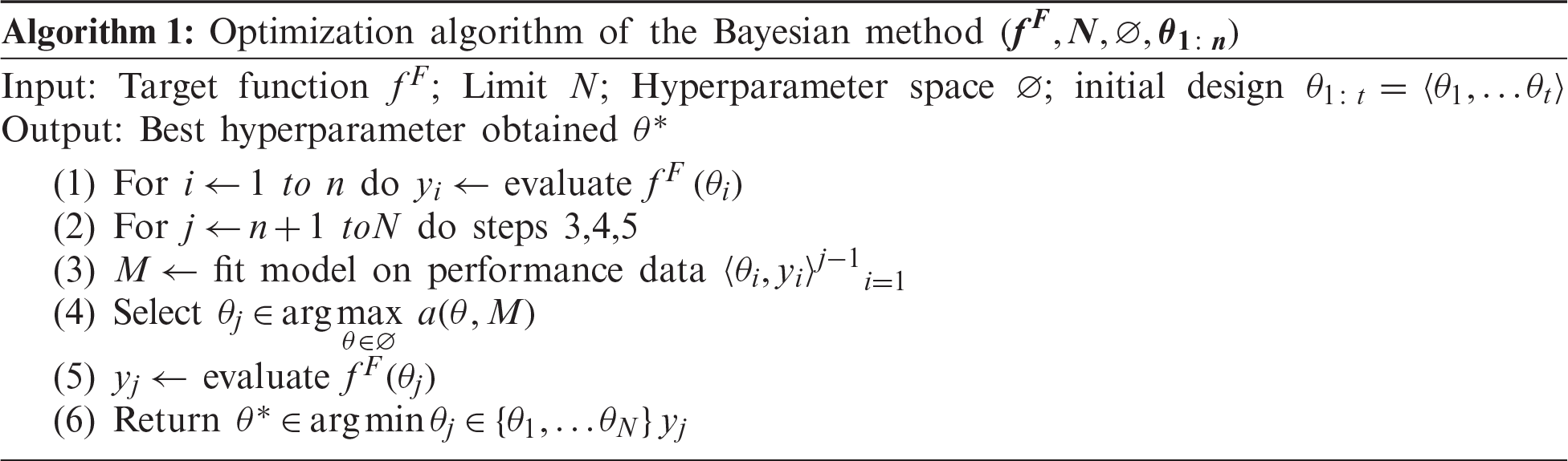
Hyperparameter tuning of an RF of decision trees is achieved using quantile error (QE), a parameter tuned for minimizing the classification error. It is required for multidimensional data such as histopathological images and Bayesian optimization [50,51].
As described in Algorithm 1, Bayesian optimization begins with function f at N values in the initial design and recording (input, output) pairs
The role of the acquisition function
Fig. 6 visualizes the change in the objective function value versus the number of function evaluations for the Bayesian optimized RF. Therein, the objective function reaches its global minimum within 30 iterations at maximum. It reiterates the BOA’s efficiency in optimizing the considered algorithms.
RF parameters were optimized using the BOA. The training set was constructed using hybrid feature variables obtained using the proposed method. Before the RF model was trained, the RF parameters were determined, including the number of trees,
Once the RF classifiers were optimized, determining the number of binary Bayesian optimized RF classifiers was important for appropriate four-class classification, as shown in Fig. 3. Hence, there is a need to build the
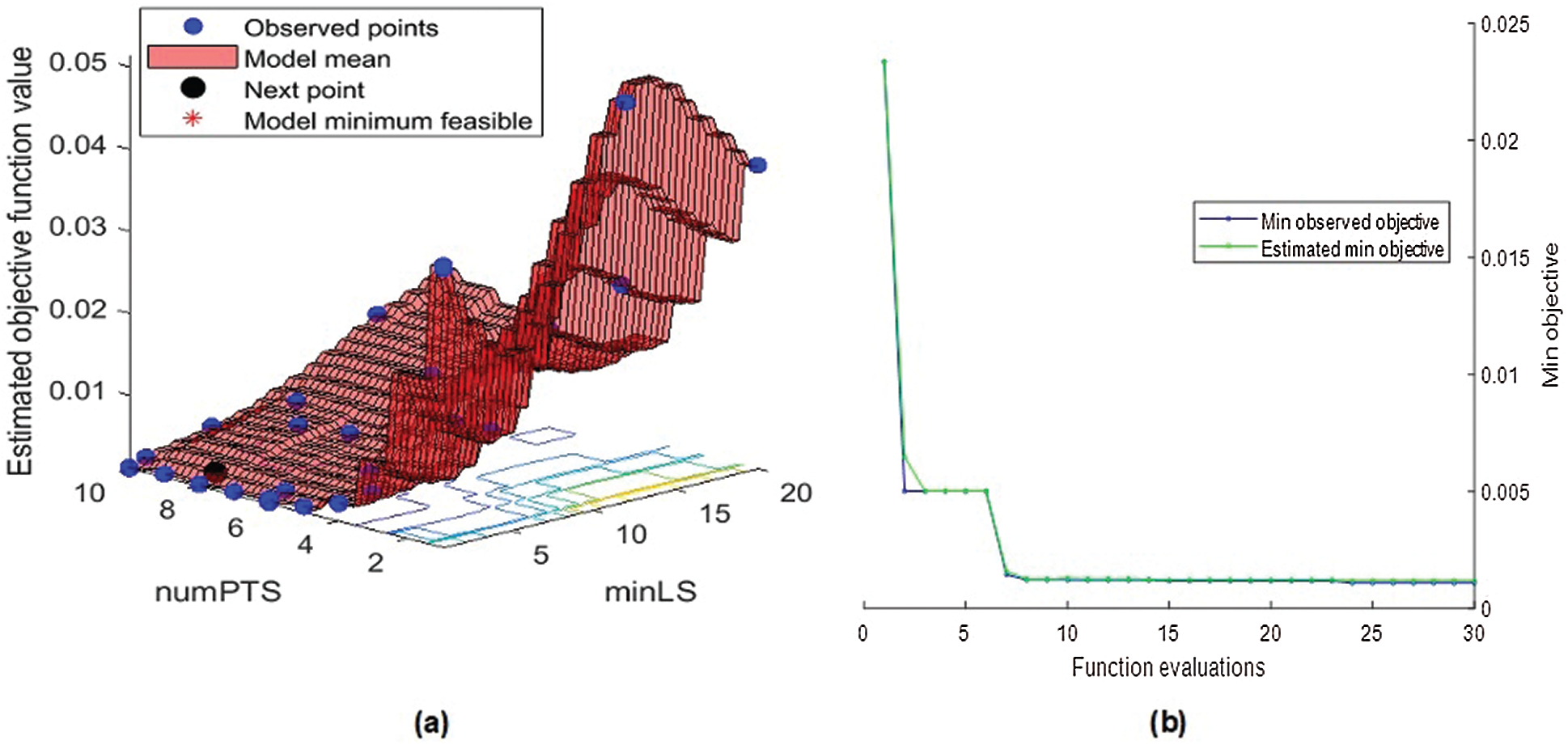
Figure 6: Bayesian optimized random forest (a) objective function model and (b) minimum objective vs. number of function evaluations
In this section, first, the performance measures used to evaluate the proposed framework are discussed. Later, the results of the proposed framework are analyzed at five levels.
The proposed system is quantitatively evaluated based on performance metrics such as accuracy, error rate, sensitivity, specificity, precision, false-positive rate, F-score, Mathew correlation coefficient (MCC), and kappa statistics described in Tab. 1. Accuracy and error rate is measured in percentage, MCC varies from −1 to +1, and rest all measures scale from 0–1 (1 is best and 0 worst) [52]. A
Table 1: Performance evaluation measures
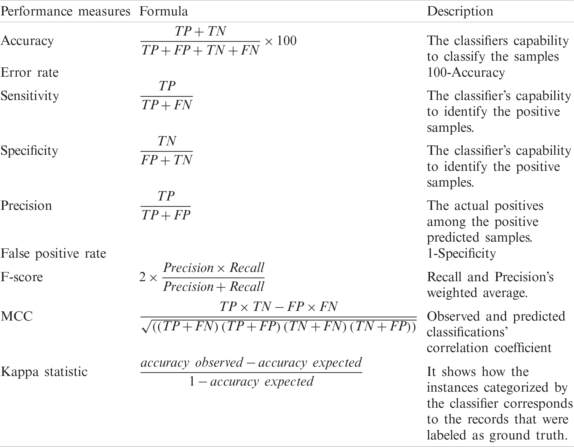
The overall MCC is determined using the technique macro-averaging for a multi-class classification. Assume 1, 2, 3, and 4 are four categories that classify the samples. Then, with the
4.2 Experimental Results and Analysis
This section analyzes the efficiency of the proposed method through different datasets and examines the findings. The results of the proposed framework were analyzed in five phases. (1) The first phase of analysis included the evaluation of the magnification-independent framework across various datasets; (2) In the second step, the model was generalized for which evaluation was done using one dataset training and another dataset testing; (3) The third phase comprised the performance analysis of the proposed framework under each considered magnification; (4) In the fourth phase, the performance and interpretation of features were analyzed; and (5) In the fifth phase of analysis, the proposed framework was compared with existing techniques, on the benchmark datasets.
4.2.1 Performance of the Proposed Colon Cancer Grading Framework
The proposed four-class colon cancer grading framework was evaluated using four different datasets, including various magnifications. To evaluate the proposed framework’s magnification-independent nature, for training and testing, colon biopsy images of various microscopic magnifications were considered from IPC (4X, 10X, and 40X microscope magnifications) and AMC (10X, 20X, and 40X microscope magnifications) datasets. Tab. 2 summarizes the performance measures of the proposed model for different datasets.
Table 2: Performance evaluation measures of the proposed framework on different datasets
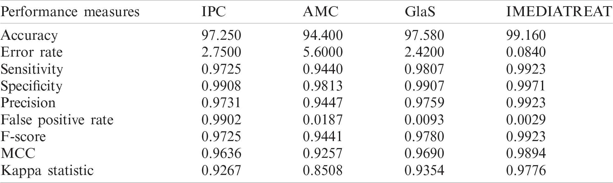
The four-class grading performed with the Bayesian optimized random forest classifier was most accurate for the IMEDIATREAT dataset, with 99.16% accuracy. In contrast, the GlaS, IPC, and AMC datasets were 97.58%, 97.25%, and 94.40% accurate, respectively. The calculated MCC was highest for the IMEDIATREAT dataset, at 0.9894, and the F-score was also higher in the IMEDIATREAT dataset, at 0.9923. The AMC dataset had the lowest MCC value (0.9257). The IMEDIATREAT dataset was most accurate with the proposed system, and the average accuracy calculated for all datasets was 97.09%. Sensitivity is an essential measure in the medical field; hence, the proposed model yields better sensitivity values of 0.9725, 0.9440, 0.9807, and 0.9923 for IPC, AMC, GlaS, and IMEDIATREAT datasets, respectively. Thus, irrespective of various magnified images considered for training and testing with IPC and AMC datasets, the proposed framework is robust across magnifications and datasets.
The

Figure 7: Confusion matrix plot for the proposed model on different datasets. (a) IPC (b) AMC (c) GlaS (d) IMEDIATREAT
A receiver operating characteristic (ROC) analysis has been conducted; the corresponding results are presented in Fig. 8. Each of the classes-normal, well, moderate, and poor, in every dataset demonstrate good ROC as the curve is toward the top left corner even though the respective class rankings vary. The IMEDIATREAT dataset exhibits better ROC for each class as all ROC curves are toward the top left corner. The ROCs across datasets reveal the robustness of the model across multiple magnifications and datasets.
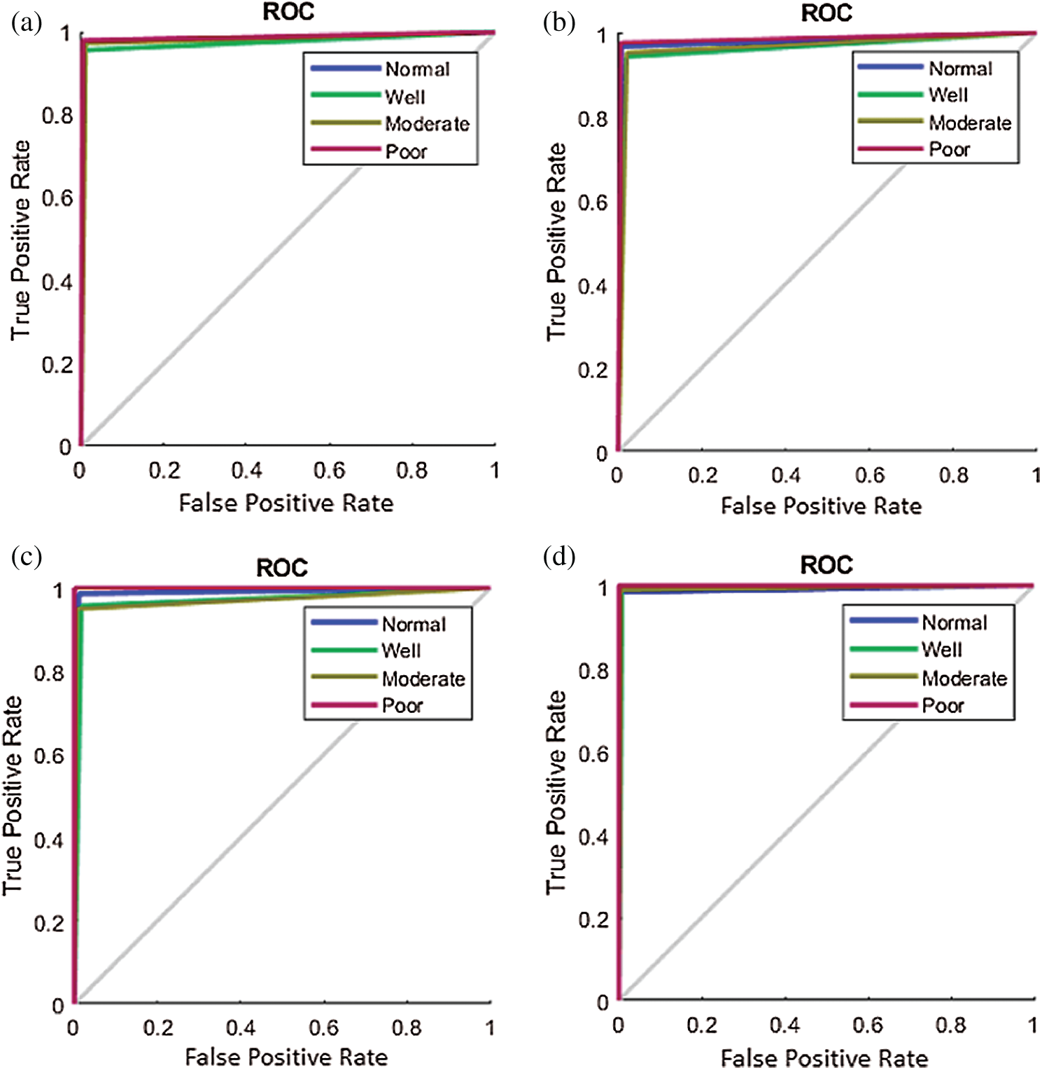
Figure 8: Receiver operating characteristic plot of the proposed framework for four classes on different datasets. (a) IPC (b) AMC (c) GlaS (d) IMEDIATREAT
4.2.2 Performance of the Proposed Model with Training on One Dataset and Testing with Another
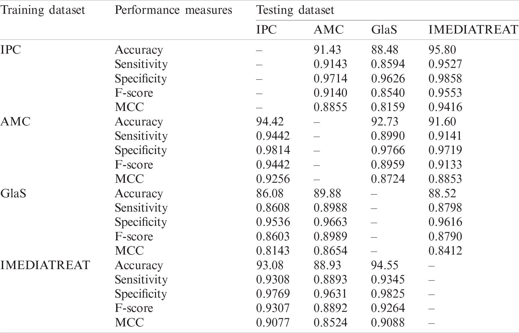
The proposed model was trained on one dataset and tested with another dataset and vice versa to assess the proposed model’s generalizability. Cross-training and testing ensure the prediction model’s performance using an unknown dataset, and the performance measures are illustrated in Tab. 3. The proposed system was evaluated for different training and testing scenarios under all magnifications. The model was trained with the IPC dataset with all magnified images, and it was tested across the AMC, GlaS, and IMEDIATREAT datasets. The highest accuracy (95.80%) was observed on the IMEDIATREAT dataset, and the accuracy on the AMC dataset (91.43%) slightly outperformed that on the GlaS dataset (88.48%). As the training was performed with 4X, 10X, and 40X images, IMEDIATREAT and AMC datasets containing 10X images exhibited considerable outperformance than other datasets, whereas the performance with the GlaS dataset was found to be on the lower side when 20X images were used for testing. Similarly, the AMC dataset comprising 10X, 20X, and 40X images were trained with the system model and tested against the IPC, GlaS, and IMEDIATREAT datasets. When tested, the IPC dataset exhibited the highest accuracy (94.42%) as the testing contained 10X and 40X images, followed by the GlaS (92.73%) and IMEDIATREAT (91.60%) datasets, in that order. GlaS and IMEDIATREAT datasets have shown comparable results as their magnifications were used for training. Subsequently, the GlaS dataset was trained and tested against the IPC, AMC, and IMEDIATREAT datasets. The highest accuracy was 89.88% for the AMC dataset, whereas the IPC dataset yielded a lower accuracy of 86.08%. Compared to other datasets, when trained with the GlaS dataset, the test datasets’ performance dipped because of the training image sets being few, single magnified, and imbalanced images across the four classes. When the IMEDIATREAT dataset containing 10X images was used for training, and IPC, AMC, and GlaS datasets were used for testing, the highest accuracy was achieved for the GlaS dataset (94.55%) because it contained a single magnification while other datasets contained multiple magnifications for testing.
Analyzing the overall statistical measures for the cross-training and testing outcome from Tab. 3 indicates the model’s generalization capability across various datasets. When trained with the IPC dataset, the average accuracy was 91.90%. Similarly, when trained with the AMC dataset, the average accuracy was 92.91%, and when trained with GlaS, the average accuracy was 88.16%; IMEDIATREAT yielded an average accuracy of 92.18%.
4.2.3 Performance Analysis of the Proposed Framework under each Magnification
To determine the supremacy of the proposed framework, the analysis under each magnification was performed for IPC and AMC datasets. The model was also tested for cross-training and testing under each magnification across datasets for generalizability.
The proposed magnification-independent framework was evaluated for each magnified image in IPC and AMC datasets. The respective magnified images were considered for training and testing to analyze each magnification’s proposed model’s performance. Tab. 4 illustrates the calculated accuracy, i.e., 94.25%, 96.50%, and 97.50% for the IPC dataset for image magnifications of 4X, 10X, and 40X, respectively. For the IPC dataset, 40X magnification provides higher accuracy than lower magnifications, whereas, in the AMC dataset, a lower magnification of 10X provides higher accuracy (98.57%). F-Scores of 0.9425, 0.9650, and 0.9749 and 0.9857, 0.9643, and 0.9447 are observed on the IPC and AMC datasets for 4X, 10X, and 40X and for 10X, 20X and 40X magnifications, respectively. For the IPC dataset, MCC at 40X was 0.9668, and it was 0.9810 in the AMC dataset at 10X magnification. The difference in data acquisition, lighting, and staining conditions can cause variation in the feature responses, thereby affecting performance across magnifications.
Tab. 5 demonstrates the proposed model’s performance accuracy when trained and tested with independent datasets at different magnifications. The model is trained with one particular magnified image of a dataset and tested with other datasets’ same magnified images. The cross-training and testing accuracy when the IPC dataset at 10X magnification was trained and tested with IMEDIATREAT was 97.20%, whereas training with IMEDIATREAT and testing with the IPC dataset at 10X magnification yields a lower accuracy (94.50%) than that obtained using the earlier dataset. Similarly, if trained with the AMC dataset at a 20X magnification and tested with GlaS, the system’s accuracy was 91.52%, and when the same process was reversed, the accuracy improved to 97.14%. The performance variation is caused by the difference in image acquisition, quality, and staining properties. When comparing the same magnification, such as 40X and training with the AMC dataset, testing with the IPC dataset achieved an accuracy of 97.25%. When training and testing were conducted vice versa, the accuracy of the system was 94.44%. Thus, even with regards to magnifications when the independent datasets are sampled for testing and training, the performance is comparable and demonstrates the model’s robustness.
Table 3: Performance measures of the proposed grading framework with cross-training and testing
4.2.4 Performance and Interpretation of Features
A quantitative and qualitative evaluation of the proposed framework for individual and combined features with accuracy and F-score is shown in Figs. 9a and 9b, respectively. For the IPC, AMC, GlaS, and IMEDIATREAT datasets, the proposed rich hybrid feature set’s average accuracy was 97.25%, 94.44%, 97.58%, and 99.16%, respectively, at the higher side. When individual features were analyzed, the cartoon feature yielded the highest accuracy for the IPC (94.40%) and IMEDIATREAT (97.22%) datasets, and for AMC and GlaS, the highest contributing features varied. Color-moment-based features exhibited a lower accuracy of fit (86.11%) for the IPC and AMC datasets. For the GlaS and IMEDIATREAT datasets, morphological features and wavelets exhibited the lowest system performances of 86.21% and 89.94%, respectively. The texture features contributed more than other features across all datasets for the grading, with accurate data fits of 96.55%, 93.10%, 95.59%, and 96.55% for the IPC, AMC, GlaS, and IMEDIATREAT datasets, respectively. The individual accuracy and F-score for color and morphological features were higher when considered separately rather than when they were combined. An accurate data fit of 90.83% (IPC), 86.11% (AMC), 90.70% (GlaS), and 89.60% (IMEDIATREAT) was found for the combination of color and morphology, which was lower than that obtained when the color and morphology features were considered separately. The texture feature combined with the morphological feature provided the next contributing features with accuracies of 95.59%, 92.86%, 94.85%, and 94.17% across the IPC, AMC, GlaS, and IMEDIATREAT datasets, respectively. Accuracy levels dropped when texture and color were combined. Thus, features, when concatenated, boost accuracy by 1%–3%. The accuracy and F-score achieved for the proposed hybrid feature are higher for all datasets when compared with the individual features.
Table 4: Performance evaluation of the proposed framework across different magnifications for the IPC and AMC datasets

Table 5: Cross-training and testing accuracy for different magnifications

Fig. 10 illustrates the mosaic plot for the different feature set distributions extracted from different datasets across magnifications. The feature distribution was plotted for the IPC, AMC, and IMEDIATREAT datasets at 10X magnification, the AMC and GlaS datasets at 20X magnification, and the IPC and AMC datasets at 40X magnification. Different grades of colon images yielded variation in the extracted features. In IPC, the healthy colon images showed less variation than other grades. The cartoon features are less sensitive toward magnification variation. They exhibited a symmetrical structure in the mosaic plot for 10X, 20X, and 40X magnifications for different colon cancer image grades. Morphological features changed at different magnifications. An evident difference existed in 10X, 20X, and 40X magnifications for different grades in different datasets. The above mosaic plots indicate feature variation for different grades for colon cancer analysis. Thus, the proposed hybrid features provide a rich classifier platform for better classification of the four-class cancer grading framework across multiple image sources.

Figure 9: (a) Accuracy and (b) F-Score for individual features and feature combinations on the proposed framework

Figure 10: Feature distribution across different magnifications for different datasets

Figure 11: Boxplot for Hybrid feature distribution across various datasets
The hybrid feature distribution across datasets in the boxplot from Fig. 11 shows the system’s performance with cross-training and testing. First, the proposed system’s hybrid feature is less skewed than other features. Skewness indicates that the data may not be normally distributed. Hence, the extracted hybrid feature has a stable distribution of data for the classifier as a training sample. Second, the IPC and AMC datasets are less skewed in the hybrid-feature-based plot. The median range is in the same range for hybrid features, ranging from 0.056 to 0.070. The IMEDIATREAT dataset variation is more favorable than those in the IPC, AMC, and GlaS datasets for the hybrid features. Thus, the median weights of the notch plots are nearly similar.
Thus, none of the features are individually adequate to separate the four classes; however, multivariate examination through machine learning precisely categorizes normal, well, moderate, and poor classes.
4.2.5 Comparison of the Proposed Model with Existing Techniques
The proposed framework’s performance is compared with existing techniques in two aspects, i.e., comparing the activation features extracted from the existing CNN models for four-class classification and comparison with existing techniques on two benchmark datasets.
In the literature [22,23,25], histopathological images were trained over existing CNN models and activation features were extracted for classification as there is scarce annotated medical data, and training from scratch requires extensive data. Commonly used existing CNN models on histopathological image data such as Alexnet [25], VGG-16 [53], Inception v3 [54], and Inception-Resnet v2 [55] are trained on the various colon image datasets to extract high-level features to classify the images into four classes, normal, well, moderate, and poor, with the Bayesian optimized RF classifier, and the comparison with the proposed magnification-independent model is illustrated in Fig. 12. The analysis shows that the proposed framework performs better than other CNN models across all datasets regarding the accuracy, sensitivity, specificity, F-score, and MCC. The high-level features extracted from the CNN models are generic features that are not specifically extracted to perform on various image magnifications and grades. The proposed robust hybrid features are meant to extract the varying texture, color, and geometric features across multiple image magnifications and grades. Inception-Resnet v2 is the best CNN model across IPC, AMC, and GlaS datasets, whereas Alexnet performs better on the IMEDIATREAT dataset. System performance across the CNN models differs as the number of levels differs in each of the networks chosen; consequently, system performance varies across the datasets. The proposed magnification-independent multiclass grading framework is a generalized framework that can work across four colon image datasets with multiple magnifications.

Figure 12: Comparison of the proposed colon cancer grading model with existing CNN models on feature learning on different datasets. (a) IPC (b) AMC (c) GlaS (d) IMEDIATREAT
Table 6: Comparison of the proposed grading framework with existing techniques on the GlaS and IMEDIATREAT datasets

Comparative analysis of the proposed framework with existing techniques on the benchmark datasets, i.e., GlaS and IMEDIATREAT datasets, is illustrated in Tab. 6. The proposed model is a four-class magnification-independent colon cancer grading framework evaluated on four different datasets with various magnifications; the accuracy of 97.58% and 99.16% were obtained for GlaS and IMEDIATREAT datasets, respectively. The performance of the proposed magnification-independent framework on GlaS dataset has surpassed previous studies [24] and [29]. However, the method presented in [17] exhibited slightly better accuracy (98.60%) than that of the proposed method because the segmentation performed is meant to work on specific magnified images (10X and 20X), and a three-class grading classification has been performed. Thus, the gland features extracted from these segmented regions are also dependent on segmentation outcomes, which are subsequently appropriate for a specific magnification and may not perform well for other low or high magnifications. Moreover, the proposed magnification-independent four-class grading framework shows better sensitivity (0.9807), specificity (0.9907), and MCC (0.9780) than the sensitivity (0.9730), specificity (0.9900), and MCC (0.9640) achieved in [17] and evaluating only the accuracy would be a biased decision. For the IMEDIATREAT dataset, the study presented in [30] developed segmentation with intensity-based thresholding, and morphological features were extracted for four-class grading to attain 89.75% accuracies; another study presented in [25] classified images into four-class using a tandem of classifiers with extracted deep CNN features on Alexnet and attained an accuracy of 98.29%. These accuracies are lesser than those acquired using the proposed method (99.16%) and evaluated under the same datasets. Sensitivity and F-score values of 0.9923 also show the proposed model’s supremacy over existing techniques on the IMEDIATREAT dataset. Thus, the proposed magnification-independent colon cancer multiclass framework is a generalized framework over multiple datasets and magnifications.
As the images are from different image sources acquired through different staining conditions, the proposed method stain normalizes images, making them uniform across datasets. The proposed framework is modeled as a magnification-independent framework evaluated to work when trained respective or irrespective of magnifications and classifies any input samples as cross-training, with testing performed across magnifications. Thus, the proposed colon cancer grading method is an effective, generalized system with an average accuracy in the range of 94.40%–99.16% across four different datasets from different country locations and various magnifications (4X, 10X, 20X, and 40X).
The proposed grading model demonstrated accurate four-class grading of colon cancer samples as an automated computational prototype. This research focuses on extracting various features, such as morphology, texture, and color for different colon image magnifications. The experimental analysis was conducted on various datasets, and the calculated outcome was satisfactory and superior to that presented in the literature. The proposed hybrid features are intended to extract all possible features for the four classes. The multi-feature-based classification method yielded better results than the individual-feature-based classification methods. Further, the proposed RF classifier hyperparameter was optimized using Bayesian optimization, which is more accurate than the traditional method. A one-vs-one strategy was adopted, ensuring an accurate outcome for multiclass classification to achieve consistent classification modeling for four-class grading. There are various advantages to our proposed system model over existing techniques. First, the proposed framework is a magnification-independent model that can work with any magnification of colon samples. Second, this algorithm requires no training and can be applied without a pre-trained model to any new specimen. Finally, the process does not require complex hardware and can be performed on desktop computers using any processor.
In particular, our approach has achieved great precision for the four-class colon cancer grading (IMEDIATREAT = 99.16% GlaS = 97.58%, IPC = 97.25% and AMC = 94.40%). Notably, the most discriminatory features emphasized by the proposed, containing cartoon features, Gabor features, color features, and morphological features, are the dominant features used to grade colon cancer samples’ malignancy. When the features were considered cumulative as a hybrid feature set, the model was less sensitive towards different magnifications and could grade the colon images more precisely.
The model was trained on a dataset from one source and tested on a dataset from another source to ensure that the proposed model was suitable for various data sources. Previous studies focused on the three-class grading of colon cancer [17,24,29] for the GlaS dataset. The results from testing the proposed grading method (Tabs. 2–5) support the four-class grading system and evidence the framework’s efficiency. The proposed classification and feature combinations herein provide a novel, reliable categorization of colorectal cancer image datasets from various sources irrespective of magnifications. The proposed model performs for any dataset input image even if it is not included in the training sample. Our proposed technology assessment shows strongly that our model functions well in typical clinical contexts where dataset samples are more varied than in controlled laboratory environments. However, the proposed method lacks the precise geometric tabulation of the cells across different grades as it is meant to work on different magnifications. The imbalanced dataset images and noise variations in the images can deteriorate the performance of the model.
The presented work proposes a magnification-independent colon cancer grading framework with a hybrid set of features, i.e., texture, color, and morphological features, and classifies images into four-class colon grades: normal, well, moderate, and poor. The proposed colon cancer grading framework includes a preprocessing phase comprising stain normalization, contrast enhancement, grayscale conversion, and K-means clustering to enhance the image quality and normalize the images across multiple datasets. The rich information regarding the image texture, edges, and structures across magnifications and grades are extracted from the texture features, including the cartoon features, Gabor wavelets, and wavelet moments. The color distribution across various grades was quantified with the color feature set comprising the HSV histogram, color auto-correlogram, and color moments. Morphological features extracted from the white cluster obtained through K-means clustering quantified the geometric variations across magnifications and grades. All extracted features were concatenated to create a rich, hybrid feature set for classification using majority voting on six Bayesian optimized RF classifiers. The experiments were conducted on four datasets with different magnification factors: IPC (4X, 10X, 40X), AMC (10X, 20X, 40X), GlaS (20X), and IMEDIATREAT (10X) to analyze the robustness of the proposed system model, wherein the IMEDIATREAT dataset calculated the highest accuracy of 99.16% followed by GlaS (97.58%), IPC (97.25%), and AMC (94.40%) datasets. Multiclass classification with optimized RF ensures the optimal accuracy of the proposed system. The proposed grading system was evaluated under various validation structures for generalizability and cross-training, and testing it as an independent model displayed promising results. In the future, magnification-independent segmentation can be implemented for grading and used to calculate and compare clinical results.
Acknowledgement: The authors thank Aster Medcity (Kochi, India) and Ishita Pathology Center (Allahabad, India) for the research’s involvement by providing quality images that are applaudable. The continuous support of Dr. Ranjana Srivastava (Ishita Pathology Center), Dr. Sarah Kuruvila (Former Senior Consultant, Aster Medcity, Kerala), and Dr. Jyotima Agarwal is highly commendable. At the time of dataset image collection, Dr. Shahin Hameed was part of Aster Medcity and has extended his valuable support throughout the research.
Funding Statement: This work was partially supported by the Research Groups Program (Research Group Number RG-1439-033), under the Deanship of Scientific Research, King Saud University, Riyadh, Saudi Arabia.
Conflicts of Interest: The authors declare that they have no conflicts of interest to report regarding the present study.
1. WHO, “Cancer.” Accessed 16 December 2020, [Online]. Available at: https://www.who.int/news-room/fact-sheets/detail/cancer. [Google Scholar]
2. F. Bray, J. Ferlay, I. Soerjomataram, R. L. Siegel, L. A. Torre et al., “Global cancer statistics 2018: Globocan estimates of incidence and mortality worldwide for 36 cancers in 185 countries,” CA: A Cancer Journal for Clinicians, vol. 68, no. 6, pp. 394–424, 2018. [Google Scholar]
3. M. Fleming, S. Ravula, S. F. Tatishchev and H. L. Wang, “Colorectal carcinoma: Pathologic aspects,” Journal of Gastrointestinal Oncology, vol. 3, no. 3, pp. 153–173, 2012. [Google Scholar]
4. W. K. Blenkinsopp, S. Stewart-Brown, L. Blesovsky, G. Kearney and L. P. Fielding, “Histopathology reporting in large bowel cancer,” Journal of Clinical Pathology, vol. 34, no. 5, pp. 509–513, 1981. [Google Scholar]
5. A. M. Khan, N. Rajpoot, D. Treanor and D. Magee, “A nonlinear mapping approach to stain normalization in digital histopathology images using image-specific color deconvolution,” IEEE Transactions on Biomedical Engineering, vol. 61, no. 6, pp. 1729–1738, 2014. [Google Scholar]
6. K. Raghesh Krishnan and S. Radhakrishnan, “Hybrid approach to classification of focal and diffused liver disorders using ultrasound images with wavelets and texture features,” IET Image Processing, vol. 11, no. 7, pp. 530–538, 2017. [Google Scholar]
7. M. N. Gurcan, L. E. Boucheron, A. Can, A. Madabhushi, N. M. Rajpoot et al., “Histopathological image analysis: A review,” IEEE Reviews in Biomedical Engineering, vol. 2, pp. 147–171, 2009. [Google Scholar]
8. N. Elazab, H. Soliman, S. El-Sappagh, S. M. R. Islam and M. Elmogy, “Objective diagnosis for histopathological images based on machine learning techniques: Classical approaches and new Trends,” Mathematics, vol. 8, no. 11, pp. 1863, 2020. [Google Scholar]
9. S. Rathore, M. Hussain and A. Khan, “Automated colon cancer detection using hybrid of novel geometric features and some traditional features,” Computers in Biology and Medicine, vol. 65, pp. 279–296, 2015. [Google Scholar]
10. S. Rathore, M. Hussain, M. Aksam Iftikhar and A. Jalil, “Novel structural descriptors for automated colon cancer detection and grading,” Computer Methods and Programs in Biomedicine, vol. 121, no. 2, pp. 92–108, 2015. [Google Scholar]
11. S. Rathore and M. Aksam Iftikhar, “CBISC: A novel approach for colon biopsy image segmentation and classification,” Arabian Journal for Science and Engineering, vol. 41, pp. 5061–5076, 2016. [Google Scholar]
12. T. Babu, D. Gupta, T. Singh and S. Hameed, “Colon cancer prediction on different magnified colon biopsy images,” in Proc. Tenth Int. Conf. on Advanced Computing, Chennai, India, pp. 277–280, 2018. [Google Scholar]
13. T. Babu, D. Gupta, T. Singh, S. Hameed, R Nayar et al., “Cancer screening on Indian colon biopsy images using texture and morphological features,” in Proc. Int. Conf. on Communication and Signal Processing, Chennai, India, pp. 0175–0181, 2018. [Google Scholar]
14. T. Babu, T. Singh, D. Gupta and S. Hameed, “Colon cancer detection in biopsy images for Indian population at different magnification factors using texture features,” in Proc. Ninth Int. Conf. on Advanced Computing, Chennai, India, pp. 192–197, 2017. [Google Scholar]
15. T. Babu, D. Gupta, T. Singh and S. Hameed, “Prediction of normal & grades of cancer on colon biopsy images at different magnifications using minimal robust texture & morphological features,” Indian Journal of Public Health Research & Development, vol. 11, no. 1, pp. 695–701, 2020. [Google Scholar]
16. E. Abdulhay, M. A. Mohammed, D. A. Ibrahim, N. Arunkumar and V. Venkatraman, “Computer aided solution for automatic segmenting and measurements of blood leucocytes using static microscope images,” Journal of Medical Systems, vol. 42, no. 4, pp. 58, 2018. [Google Scholar]
17. S. Rathore, M. A. Iftikhar, A. Chaddad, T. Niazi, T. Karasic et al., “Segmentation and grade prediction of colon cancer digital pathology images across multiple institutions,” Cancers, vol. 11, no. 11, pp. 1700, 2019. [Google Scholar]
18. K. Sirinukunwattana, D. R. J. Snead and N. M. Rajpoot, “A stochastic polygons model for glandular structures in colon histology images,” IEEE Transactions on Medical Imaging, vol. 34, no. 11, pp. 2366–2378, 2015. [Google Scholar]
19. S. Husham, A. Mustapha, S. Mostafa, M. Al-Obaidi, M. Mohammed et al., “Comparative analysis between active contour and otsu thresholding segmentation algorithms in segmenting brain tumor magnetic resonance imaging,” Journal of Information Technology Management, vol. 12, pp. 48–61, 2020. [Google Scholar]
20. I. J. Hussein, M. A. Burhanuddin, M. A. Mohammed, M. Elhoseny, B. Garcia-Zapirain et al., “Fully automatic segmentation of gynaecological abnormality using a new viola-jones model,” Computers, Materials & Continua, vol. 66, no. 3, pp. 3161–3182, 2021. [Google Scholar]
21. A. Janowczyk and A. Madabhushi, “Deep learning for digital pathology image analysis: A comprehensive tutorial with selected use cases,” Journal of Pathology Informatics, vol. 7, pp. 29, 2016. [Google Scholar]
22. P. Kainz, M. Pfeiffer and M. Urschler, “Semantic segmentation of colon glands with deep convolutional neural networks and total variation segmentation,” ArXiv, arXiv: 1511.06919, vol. 5, pp. e3874, 2015. [Google Scholar]
23. Y. Xu, Z. Jia, L. Wang, Y. Ai, F. Zhang et al., “Large scale tissue histopathology image classification, segmentation, and visualization via deep convolutional activation features,” BMC Bioinformatics, vol. 18, pp. 281, 2017. [Google Scholar]
24. R. Awan, K. Sirinukunwattana, D. Epstein, S. Jefferyes, U. Qidwai et al., “Glandular morphometrics for objective grading of colorectal adenocarcinoma histology images,” Scientific Reports, vol. 7, pp. 16852, 2017. [Google Scholar]
25. D. Lichtblau and C. Stoean, “Cancer diagnosis through a tandem of classifiers for digitized histopathological slides,” PLOS ONE, vol. 14, no. 1, pp. 1–20, 2019. [Google Scholar]
26. F. A. Spanhol, L. S. Oliveira, C. Petitjean and L. A. Heutte, “Dataset for breast cancer histopathological image classification,” IEEE Transactions on Biomedical Engineering, vol. 63, no. 7, pp. 1455–1462, 2016. [Google Scholar]
27. O. Iizuka, F. Kanavati, K. Kato, M. Rambeau, K. Arihiro et al., “Deep learning models for histopathological classification of gastric and colonic epithelial tumours,” Scientific Reports, vol. 10, pp. 12, 2020. [Google Scholar]
28. J. Kather, C. A. Weis, F. Bianconi, S. M. Melchers, L. R. Schad et al., “Multi-class texture analysis in colorectal cancer histology,” Scientific Reports, vol. 6, pp. 27988, 2016. [Google Scholar]
29. B. Saroja and A. S. Priyadharson, “Adaptive pillar k-means clustering-based colon cancer detection from biopsy samples with outliers,” Computer Methods in Biomechanics and Biomedical Engineering Imaging & Visualization, vol. 7, no. 1, pp. 1–11, 2019. [Google Scholar]
30. D. Boruz and C. Stoean, “On supporting cancer grading based on histological slides using a limited number of features,” Annals of the University of Craiova, Mathematics and Computer Science Series, vol. 45, no. 1, pp. 156–165, 2018. [Google Scholar]
31. C. Stoean, R. Stoean, A. Sandita, D. Ciobanu, C. Mesina et al., “Svm-based cancer grading from histopathological images using morphological and topological features of glands and nuclei,” in Proc. Intelligent Interactive Multimedia Systems and Services, pp. 145–155, 2016. [Google Scholar]
32. A. Nawandhar, N. Kumar, V. R and L. Yamujala, “Stratified squamous epithelial biopsy image classifier using machine learning and neighborhood feature selection,” Biomedical Signal Processing and Control, vol. 55, pp. 101671, 2020. [Google Scholar]
33. S. Rathore, T. Niazi, M. A. Iftikhar and A. Chaddad, “Glioma grading via analysis of digital pathology images using machine learning,” Cancers, vol. 12, no. 3, pp. 578, 2020. [Google Scholar]
34. S. Roy, S. Lal and J. R. Kini, “Novel color normalization method for hematoxylin eosin stained histopathology images,” IEEE Access, vol. 7, pp. 28982–28998, 2019. [Google Scholar]
35. H. O. Lyon, A. P. De Leenheer, R. W. Horobin, W. E. Lambert, E. K. Schulte et al., “Standardization of reagents and methods used in cytological and histological practice with emphasis on dyes, stains and chromogenic reagents,” The Histochemical Journal, vol. 26, no. 7, pp. 533–544, 1994. [Google Scholar]
36. S. Rathore, M. Hussain, M. Aksam Iftikhar and A. Jalil, “Ensemble classification of colon biopsy images based on information rich hybrid features,” Computers in Biology and Medicine, vol. 47, pp. 76–92, 2014. [Google Scholar]
37. M. B. Amin, F. L. Greene, S. B. Edge, C. C. Compton, J. E. Gershenwald et al., “The eighth edition AJCC cancer staging manual: continuing to build a bridge from a population-based to a more “personalized” approach to cancer staging,” CA: A Cancer Journal for Clinicians, vol. 67, no. 2, pp. 93–99, 2017. [Google Scholar]
38. K. Zuiderveld, Contrast Limited Adaptive Histogram Equalization. USA: Academic Press Professional, Inc., pp. 474–485, 1994. [Google Scholar]
39. K. Fukunaga and L. Hostetler, “The estimation of the gradient of a density function, with applications in pattern recognition,” IEEE Transactions on Information Theory, vol. 21, no. 1, pp. 32–40, 1975. [Google Scholar]
40. L. Chang, X. Feng, X. Zhu, R. Zhang, R. He et al., “CT and MRI image fusion based on multiscale decomposition method and hybrid approach,” IET Image Processing, vol. 13, no. 1, pp. 83–88, 2019. [Google Scholar]
41. S. Thomas and A. Vijayan, “Automated colon cancer detection using kernel sparse representation based classifier,” International Journal of Engineering and Advanced Technology, vol. 4, no. 6, pp. 317–321, 2015. [Google Scholar]
42. G. Wimmer, T. Tamaki, J. Tischendorf, M. Häfner, S. Yoshida et al., “Directional wavelet based features for colonic polyp classification,” Medical Image Analysis, vol. 31, pp. 16–36, 2016. [Google Scholar]
43. M. Kherfi, D. Ziou and A. Bernardi, “Combining positive and negative examples in relevance feedback for content-based image retrieval,” Journal of Visual Communication and Image Representation, vol. 14, no. 4, pp. 428–457, 2003. [Google Scholar]
44. J. Huang, S. R. Kumar, M. Mitra, W.-J. Zhu and R. Zabih, “Image indexing using color correlograms,” in Proc. IEEE Computer Society Conf. on Computer Vision and Pattern Recognition, San Juan, Puerto Rico, USA, pp. 762–768, 1997. [Google Scholar]
45. X. Min, M. Li, D. Dong, Z. Feng, P. Zhang et al., “Multi-parametric MRI-based radiomics signature for discriminating between clinically significant and insignificant prostate cancer: cross-validation of a machine learning method,” European Journal of Radiology, vol. 115, no. 6, pp. 16–21, 2019. [Google Scholar]
46. M. Zahangir Alam, M. Saifur Rahman and M. Sohel Rahman, “A random forest based predictor for medical data classification using feature ranking,” Informatics in Medicine Unlocked, vol. 15, 100180, pp. 1–12, 2019. [Google Scholar]
47. M. Zakariah, “Classification of large datasets using random forest algorithm in various applications: survey,” International Journal of Engineering and Innovative Technology, vol. 4, no. 3, pp. 189–198, 2014. [Google Scholar]
48. D. Trehan, “Why choose random forest and not decision trees,” Towards AI—Multidisciplinary Science Journal, 2020. [Online]. Available at: https://towardsai.net/p/machine-learning/why-choose-random-forest-and-not-decision-trees. [Google Scholar]
49. W. M. Czarnecki, S. Podlewska and A. J. Bojarski, “Robust optimization of SVM hyperparameters in the classification of bioactive compounds,” Journal of Cheminformatics, vol. 7, no. 38, pp. 1–15, 2015. [Google Scholar]
50. J. Wu, X.-Y. Chen, H. Zhang, L.-D. Xiong, H. Lei et al., “Hyperparameter optimization for machine learning models based on bayesian optimization,” Journal of Electronic Science and Technology, vol. 17, no. 1, pp. 26–40, 2019. [Google Scholar]
51. N. Meinshausen, “Quantile regression forests,” Journal of Machine Learning Research, vol. 7, no. 35, pp. 983–999, 2006. [Google Scholar]
52. J. B. Reitsma, A. S. Glas, A. W. Rutjes, R. J. Scholten, P. M. Bossuyt et al., “Bivariate analysis of sensitivity and specificity produces informative summary measures in diagnostic reviews,” Journal of Clinical Epidemiology, vol. 58, no. 10, pp. 982–990, 2005. [Google Scholar]
53. H. Chougrad, H. Zouaki and O. Alheyane, “Convolutional neural networks for breast cancer screening: Transfer learning with exponential decay,” Computer Methods and Programs in Biomedicine, vol. 157, pp. 19–30, 2019. [Google Scholar]
54. H. M. Ahmad, S. Ghuffar and K. Khurshid, “Classification of breast cancer histology images using transfer learning,” in Proc. 16th Int. Bhurban Conf. on Applied Sciences and Technology, Islamabad, Pakistan, pp. 328–332, 2019. [Google Scholar]
55. S. Christian, S. Ioffe, V. Vanhoucke and A. Alemi, “Inception-v4, inception-resnet and the impact of residual connections on learning,” in Proc. Thirty-first AAAI Conf. on Artificial Intelligence (AAAI’17), California, USA: San Francisco, pp. 4278–4284, 2016. [Google Scholar]
 | This work is licensed under a Creative Commons Attribution 4.0 International License, which permits unrestricted use, distribution, and reproduction in any medium, provided the original work is properly cited. |