DOI:10.32604/cmc.2021.017062
| Computers, Materials & Continua DOI:10.32604/cmc.2021.017062 | |
| Article |
Adaptive Power Control Aware Depth Routing in Underwater Sensor Networks
1Department of Computer Science, FAST National University of Computer and Emerging Sciences (NUCES), Karachi, Pakistan
2Dr. A. Q. Khan Institute of Computer Sciences and Information Technology, Kahuta, Pakistan
3Faculty of Computer Science and Information Technology, University of Malaya, Kuala Lumpur, 50603, Malaysia
4Department of Computer Science, COMSATS University Islamabad, Islamabad, Pakistan
5Deanship of Scientific Research, King Saud University, Riyadh, Saudi Arabia
6Department of Information Technology, College of Computer and Information Technology, Taif University, Taif, 21944, Saudi Arabia
7Faculty of Computing and Informatics, Universiti Malaysia Sabah, Kota Kinabalu, Sabah, Malaysia
*Corresponding Author: Ag Asri Ag Ibrahim. Email: awgasri@ums.edu.my
Received: 20 January 2021; Accepted: 07 March 2021
Abstract: Underwater acoustic sensor network (UASN) refers to a procedure that promotes a broad spectrum of aquatic applications. UASNs can be practically applied in seismic checking, ocean mine identification, resource exploration, pollution checking, and disaster avoidance. UASN confronts many difficulties and issues, such as low bandwidth, node movements, propagation delay, 3D arrangement, energy limitation, and high-cost production and arrangement costs caused by antagonistic underwater situations. Underwater wireless sensor networks (UWSNs) are considered a major issue being encountered in energy management because of the limited battery power of their nodes. Moreover, the harsh underwater environment requires vendors to design and deploy energy-hungry devices to fulfil the communication requirements and maintain an acceptable quality of service. Moreover, increased transmission power levels result in higher channel interference, thereby increasing packet loss. Considering the facts mentioned above, this research presents a controlled transmission power-based sparsity-aware energy-efficient clustering in UWSNs. The contributions of this technique is threefold. First, it uses the adaptive power control mechanism to utilize the sensor nodes’ battery and reduce channel interference effectively. Second, thresholds are defined to ensure successful communication. Third, clustering can be implemented in dense areas to decrease the repetitive transmission that ultimately affects the energy consumption of nodes and interference significantly. Additionally, mobile sinks are deployed to gather information locally to achieve the previously mentioned benefits. The suggested protocol is meticulously examined through extensive simulations and is validated through comparison with other advanced UWSN strategies. Findings show that the suggested protocol outperforms other procedures in terms of network lifetime and packet delivery ratio.
Keywords: UWSNs; UASNs; QoS
In addition to this study’s motivations, this section provides a brief overview and introduction to underwater wireless sensor networks (UWSNs) highlights the contributions of this study, and describes the structure of the paper.
Water can be found almost everywhere in the world. It covers approximately 70% of the earth. Underwater environments are incredibly essential for human existence. Research focuses on underwater elements because of the decrease in terrestrial methods. UWSNs remain as researchers’ interests because of their capability to screen underwater environments. UWSNs are broadly utilized in coastline observation and assurance, sea calamity anticipation, observing of underwater contamination, military protection, route assistance, checking of marine oceanic environment, and underwater asset investigation [1]. The use of protocols intended for terrestrial wireless sensor networks (TWSNs) in the underwater environment is ineffective [2]. TWSNs and UWSNs are different in numerous ways. For example, in underwater, acoustic links are more utilized than radio links. The UWSN topology is more challenging than TWSN topology because underwater nodes move unreservedly with water streams. The former is also more dynamic than the latter, thereby causing their positions to change most of the time. The localization of nodes in UWSNs is more complicated than that in TWSNs. The positioning of nodes in UWSNs is sparse, and charging them after they are positioned is difficult [1,3].
Moreover, UWSNs face other challenges, such as low bandwidths, that result in low data rates. The available underwater bandwidth is 40 kbps. The low propagation speed results in high delay. Underwater propagation speed is almost 1500 m/s or essentially 5 times less than the radio waves [4,2]. Underwater nodes face high mobility that results in network topology instability. Energy constraints caused by difficulty in replacing the batteries are noted. The bit error rate is also high. After a thorough investigation of existing UWSN routing schemes, some major observations regarding the energy hole problem, decreased packet delivery ratio (PDR), and maximum load upon any sensor node near the sink are noted. The concluding remarks are summarized as follows:
a) Most existing routing schemes employ sensor nodes’ peak transmission power while transmitting packets to neighboring nodes or sinks. This mechanism results in the rapid energy consumption of sensor nodes. Moreover, high transmission power utilization creates more channel interferences [5,6]. Consequently, the probability of energy hole creation is also increased.
b) The unbalanced load distribution of forwarding data results in the rapid reduction of node energy and creates energy holes in the network. Owing to the occurrence of energy hole, various sensor nodes die prior to their rest. This energy hole problem results in increased energy consumption and decreased network lifetime [5].
c) The existing schemes cannot avoid additional load on nodes near the sink node. Thus, any node near the sink expends its energy faster than those positioned away from the sink node. Consuming energy rapidly also decreases the PDR [5,7].
d) A majority of the existing UWSN considers the use of one or multiple static sinks on the water’s surface. These sinks acquire data from sensor nodes using different routing mechanisms. This approach poses great problems in scalability when the network size is increased. Moreover, it creates a bottleneck and lowers the performance of the network. Additionally, the nodes closer to these sinks deplete their energy very rapidly and create energy holes that force the rest of the nodes into distant communication and results in rapid energy depletion. Thus, the overall network lifetime is reduced.
Most of the techniques do not apply the mechanism of adaptive transmission power control. Furthermore, they work well in most situations. However, in extreme underwater environment where a lot of disturbances, fading and noises, unwanted failures, interferences, and collisions occur, the use of maximum transmission power slows down the performance of the network. Thus, a routing scheme that utilizes minimum transmission power must be proposed to improve the lifetime, PDR, and interference of the network. The routing protocol that is being proposed in this work minimizes channel interference and reduces energy consumption in sparse areas using an adaptive communication power control mechanism. Furthermore, in dense regions, clustering is implemented to decrease repetitive transmissions. By contrast, mobile sinks (MSs) are used to gather information for minimum energy consumption.
Underwater wireless sensor networks (UWSN) elicit considerable attention in academic, research, and industrial fields. Reduction of energy depletion of sensor nodes improves the network life of UWSNs, which in turn decreases the overall network cost [4,6], because several applications, such as coastline observation and assurance, sea calamity anticipation, observation of underwater contamination, military protection, and route assistance, and checking the marine oceanic environment and underwater asset investigation, are applied in this domain [4,1]. The probability of creating void holes is significantly reduced, whereas transmission reliability and end-to-end delay are improved effectively [4,8]. The success of all UWSN applications depends on the efficiency of the routing protocols that influence the entire services of UWSNs. Existing protocols, such as sparsity-aware energy-efficient cluster (SEEC), CSEEC, and CDSEEC, are energy-efficient routing protocols. However, some major observations regarding the energy hole problem, decreased PDR, and maximum load on sensor nodes closer to the sink in the aforementioned protocols were noted.
• First, an unbalanced load for forwarding data results in the rapid reduction of node energy, known as the energy hole. Owing to the occurrence of energy hole, various sensor nodes die prior to their rest. This energy hole problem increased energy consumption and decreased network lifetime [5].
• Second, these existing schemes cannot avoid additional load on nodes closer to the sink node. Nodes closer to the sink devour their energy rapidly than nodes positioned away from the sink node because of the large load. Therefore, consuming energy rapidly also decreases the PDR [5,7].
• Third, these schemes use maximum transmission power to reduce network performance [5,6].
This research presents a controlled transmission power-based SEEC (CTPSEEC) protocol in UWSNs. The contributions of the proposed protocol is threefold. It uses the adaptive power control mechanism to utilize sensor nodes’ battery and reduce channel interference efficiently. Moreover, thresholds are defined to ensure a successful communication.
Furthermore, clustering is implemented in dense regions to decrease the repetitive transmissions that affect nodes and interference’s energy consumption ultimately. Additionally, MSs are deployed to gather information locally to achieve the previously mentioned benefits.
Most techniques do not use the mechanism of adaptive transmission power control. Furthermore, they work well in ultimate situations. However, in an extreme underwater environment, where a lot of disturbance, fading and noises, unwanted failures, interference, and collision occur, the use of maximum transmission power slows down the performance of the network. Therefore, a type of routing scheme that utilizes minimum transmission power must be proposed to improve the network lifetime, PDR, and interference. This routing protocol is being proposed to minimize channel interference and reduce energy consumption in sparse areas using an adaptive communication power control mechanism.
Furthermore, in dense regions, clustering is implemented to decrease repetitive transmissions. By contrast, MSs are used to gather minimum energy consumption information. The advantages of our proposed protocol can be summarized as follows:
• Channel interference that ultimately increases the network lifetime reduces the interference and avoids the energy hole creation.
• The clustering technique is incorporated in dense regions to reduce the duplication of transmitted packets and balance the load of data packets that potentially reduces the interference and improves the battery usage of sensor nodes.
• Deployment of MSs to collect the packets for enhancing the network lifetime locally by reducing transmission distance and minimizing the interference. Moreover, it helps avoid energy holes and increases successful packet delivery.
The rest of this paper is organized as follows:
Section 2 presents the background and classification of the routing protocol of UWSNs. Section 3 discusses the state-of-the-art work related to this article’s focus area. Section 4 presents the proposed solution.
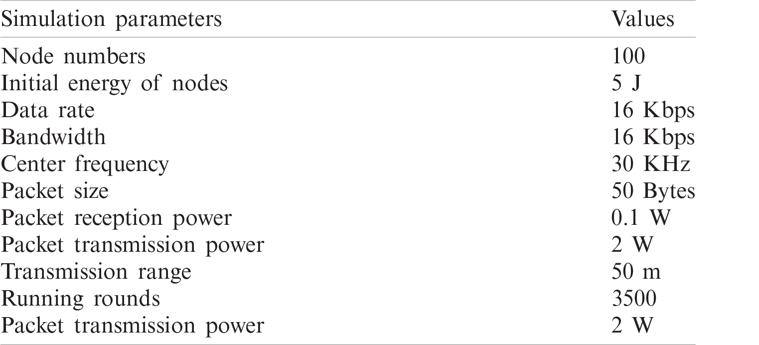
Section 5 explains the simulation setup. Section 6 presents the performance evaluation of the proposed scheme in terms of network lifetime, stability period, residual energy, packets received per round, and total packets received at the sink. The proposed protocol is evaluated on the basis of the following metrics: network lifetime and packets received per round residual energy. To verify the proposed scheme, rigorous comparison with current state-of-the-art schemes is conducted with depth-based routing protocol (DBR), energy-efficient DBR (EEDBR), and SEEC underwater routing schemes by using simulation parameters, as shown in Tab. 1. The proposed scheme is also evaluated. Section 7 concludes the paper and provides future directions to work in this domain.
Table 1: Simulation parameters used for CTP-SEEC performance evaluation
In this section, some of the concepts aside from the existing routing approaches in UWSNs are discussed briefly. These concepts are grouped according to their characteristics and functions; the authors classified and discussed the routing protocols as non-localization, localization-aware, and clustering-based protocols (Fig. 1) as follows:
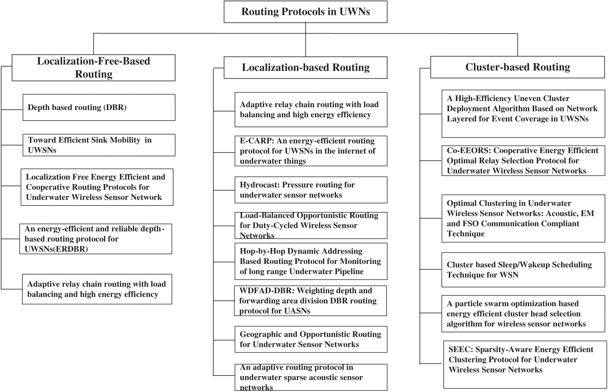
Figure 1: Taxonomy of routing protocols in UWSN
2.1 Localization-Free Routing Strategies
This class contains strategies that do not need prior geographical knowledge of the network. The strategies implement processes without requiring the position information of other nodes. Prior geographical knowledge of the network in such strategies is not needed. Such strategies are mostly targeted toward flooding events. These strategies are viewed as having a fast packet delivery rate and minimum E2E delay.
In DBR [9], previous network knowledge is not required. The protocol selects the sensor node with the lowest depth to be assigned to the router and the packet. The protocol functions by comparing the transmitter node’s depth with that of the receiving node. If the transmitter depth exceeds that of the receiver, then the data will be forwarded. Otherwise, then the node will not be selected. Likewise, in EE-DBR, the depth information and remaining energy are assigned to the node during data communication. DBR, as a routing protocol, controls dynamic networks proficiently. It also needs node depth data to pass packets toward the sink. Every confirmed node sends the packet based on transmitter nodes depth and includes what was previously unsent in the same packet. The network lifetime is improved in DBR and results in high PDR. However, the network becomes partitioned, and useful resources are not utilized [10].
Authors in [11] proposed “Localization-Free Energy-Efficient Routing (LFEER)” first and “Localization-Free Energy-Efficient Cooperative Routing (CO-LFEER)” second. The former is used to select a node based on its remaining energy, hops, and link bit error rate, on which data packets are being transmitted. For the latter, some replicas of data are received by the sink to determine the data’s quality. These schemes provide better outcomes concerning energy and increased PDR. However, the exact positions of sensor nodes in these schemes are unknown, thereby resulting in computational complexity and additional use of resources. Considering the restrictions in UWSN, energy-efficient schemes are more preferred. Underwater sensors are used for various application frameworks, and a different approach is taken when suggesting a contemporary routing schema [12].
2.2 Localization-Aware Routing Strategies
This class of routing strategies commonly require the geographical updates of all nodes and sink positions. These strategies are supposed to be energy effective. However, most of the energy is wasted during the collection of geographical updates. The registrations are frequently modified because the nodes’ location may shift due to water flow. In localization-aware routing protocols, a node requests information from every node in the network and the sink. This framework requires former network data to function. In [13], the researchers suggested the use of mobile sensor nodes to reduce the issue of energy holes and keep the sink fixed. To fulfil this objective, clusters are formed in the network, and data gathering is carried out using mobile nodes. This strategy ensures energy proficiency, improved network lifetime, and load maximization. However, this scheme has to compensate by having high end-to-end delay. Likewise, authors in [14] proposed a dispersed cross-layer reactive routing protocol. This technique addresses most of the CARP scheme’s known issues, where the researchers ignored the re-usability propriety, thereby enhancing network lifetime and reduces how much energy is expended by eliminating the need for control packets. This strategy leads to lesser throughput and higher path loss because of the nodes’ continuous movement. Then, in [15], the authors aim to create an effective routing algorithm that can broadcast to any of the sink nodes while solving the energy hole problem consistently. However, this protocol is limited because its performance is relatively ineffective, and it increases overhead and energy consumption. In the article, although the authors consider the depth of the present node and the forwarding node to reduce the possibility of void holes and energy expenditure, sending packets via two hops does not eliminate the problem yet.
Similarly, in [4], the authors used a scheme that worked by changing the pipeline’s radius and forearming the forwarding area, thereby reducing the occurrence of replicated packets. This instance leads to enhanced PDR, reduced energy expenditure, and low end-to-end latency. However, the void hole issue still exists. Additionally, in [16], the authors designed non-synchronous duty-cycled wireless sensor networks. To estimate the best forwarding core calculation and consider residual energy, the protocol considers load balancing, coverage loss, and connectivity to select the forwarding node. However, asynchronous duty cycling results in delays. Hence, we need to wait for the next-hop node to wake up because the duty cycling in this protocol is higher than what is necessary. In [2], the authors proposed a routing scheme that forwarded data toward the destination node. To avoid duplication in GEDAR, the nodes on lower priority suppress their packet transmission. The important feature of this protocol is that it uses a depth adjustment scheme when a void hole occurs (i.e., when a void node exists, it is transferred to a different depth so that forwarding can resume). The use of this scheme enhanced the performance of the network because it avoids the void hole successfully. However, moving nodes toward new depth results in unnecessary energy expenditure and higher end-to-end latency.
Furthermore, in [17], the researchers proposed a strategy that used dynamic addressing. This study supports the selection of a suitable hop node. This approach assigns hop addresses to each node that helps in forwarding data. Although this protocol increases the PDR, it also results in high-energy consumption.
2.3 Cluster-Based Routing Protocols
A clustered-based routing protocol on node mobility is established to indicate a cluster’s structure. This technique improves the cluster head (CH) nodes and cluster-element nodes. CH nodes gather information from clustered element nodes and pass it to the sink nodes. The presented study defines each cluster-based routing protocol based on node mobility, as described below. In [17], assembly projects are proposed to reduce data loading on the basin. Their aggregation schemes are based on data collection that are distributed on the basis of the network’s local distribution. The CHs are nominated on the basis of the high residual energy between neighboring nodes. After electing the head of the block, all node members within the head node’s contact range begin data transmission, subsequently, it is assembled into a composite package. After the assembly, the vehicle data packet is transmitted to the destination over the header node. In hierarchical routing, aggregation, energy consumption, and passing load at the base station are minimized. However, the local group’s result shows a time problem, that is, nodes perform with increased end-to-end latency. As a result, the use of cluster routing in time-sensitive applications is inadequate for UWSNs. Additionally, authors in [7] proposed sparsity-aware energy-efficient clustering (SEEC) strategy for UWSNs. SEEC specifically searches for sparse areas in the network. Mostly, underwater network regions become sparse because of the water current and the high cost of manufacture, design, and deployment of sensors for broadcasting. They split the network area into equal sub-areas and find sparse and dense network sites using the dense and sparse algorithms, respectively [18].
SEEC makes the network efficient by moving the sink in scattered areas and clustering in dense regions. SEEC also ensures network stabilization with the best clustering in densely populated areas, where each logically dense site represent a fixed set. SEEC reduces network power consumption by distributing load via static clustering in dense network areas uniformly. In this way, it achieves a better network lifetime. However, it does not assure better control in sparse regions. By having improved equal load distribution, all of the sensor nodes of UWSNs can achieve extreme stability and network lifetime.
Fig. 2 shows the splitting of network site into left and rightareas. Here, the terms of selecting the CH in SEEC routing protocol is presented as follows [1]
where
The node with low depth and high energy level is chosen as CH. The authors proposed a “cooperative energy-efficient optimal relay selection protocol” for wireless underwater sensor networks in [19]. Moreover, a source node selects a relay node and a sink node by itself and then sends data to the sink node through the relay node.
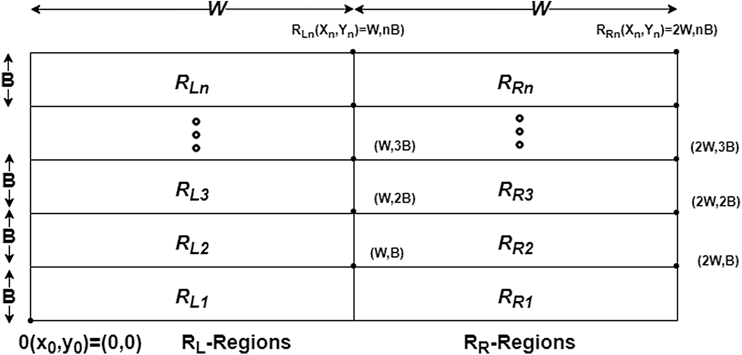
Figure 2: Network site partition scenario [7]
This method eliminates the necessity of synchronization among the source, relay, and sink nodes. Furthermore, the sink transfers the acknowledgement to the source node to receive or re-transmit the data. Hence, this scheme adds in a fewer amount of packet drops. However, the data load on the source, relay, and sink node may increase or reduce the nodes’ stability period. The authors in [20] also proposed an energy dissipation model of FSO and EM to scan the analytical framework and obtained the optimal range of clusters for Gaussian-distributed UWSNs. Logical results are calculated by relocating the sink to three positions: center, corners, and middle point of the sensing area. Thus, a minimum energy expenditure is observed. However, it also causes higher end-to-end latency. To conserve energy, cluster-based sleep–wake scheduling is proposed.
For instance, in [21], the researchers used a method whereby some of the nodes are assigned the role of initiator nodes and are tasked with selecting the CH. The CH node that contains the highest remaining power level is chosen as the CH. The head node is activated while the other nodes are switched to sleep mode. The head node is selected, and then transmission is continued toward the sink node. This technique reduces energy consumption and increases the lifetime and PDR. In [21], the authors first perform a theoretical analysis to obtain the network’s expected value. Next, they divide the network into irregular clusters. They employ the strategy of recovery balance consumption of energy among clusters. This study achieved enhanced PDR, reduced energy consumption, and extended network lifetime. However, this scheme results in network variation. The author proposes particle encoding and fitness function [22] to develop this algorithm. The authors focus on different parameters, such as the distance among the clusters, the distance among sink nodes, and the remaining nodes’ energy inside the clusters to enhance energy efficiency. Finally, high PDR and increased lifetime and energy efficiency are achieved. “Adaptive FFC/FWD and FEC/ARQ” structures for clustering in WSNs are proposed [23] to test the pay-off among consistency and energy effectiveness. This scheme focuses on the channel’s condition and the distance among the nodes. This scheme results in a more reliable and more energy-efficient network. However, this scheme is only effective for small networks. It addresses the issues pointed out in various aforementioned UWSN routing schemes and improves network performance by balancing the load distribution, lowering the channel interference, achieving energy efficiency, and avoiding the network’s energy holes by integrating the clustering, utilizing MSs, and transmitting power control mechanisms. Different routing protocols have been accurately reviewed in terms of node mobility, data forwarding, route discovery, route maintenance, and performance issues. In addition, the focus is placed on the execution of reviewed routing protocols via a well-organized approach. We have studied a number of cluster-based routing protocols for energy-efficient WSN. The guidance provided in this section would be beneficial for the researchers to work in this field.
This study focused on efficient energy expenditure by using sensor nodes at sparse areas with the free location of high mobility sensor nodes underwater. After reviewing several routing protocols and classifying them as location-free and location-aware protocols, DBR, EEDBR, and SEEC are proposed to reduce the energy consumed by the sensor nodes during data transmission. We compare the implementation among these energy-efficient location-free routing protocols in UWSN. We found that DBR and EEDBR work quite well in dense areas in the network. However, they do not work well in sparse areas.
In DBR [9], transmitter sensor nodes are selected on the basis of depth metric by multi hopping using a greedy approach, which fails in sparse networks. As long as it has no specific strategy for efficient route election (just depth criteria), the same path is chosen every time to transmit information to the sink by a source node. In this way, the nodes in the selected routing path will die, thereby leading to void region creation, which reduces network life. Similarly, in EEDBR [24], the remaining energy is used to select the forwarder node as a second metric. Hence, sensor nodes with lower depth and higher remaining energy expend their energy faster than those away from the sink, thereby increasing the problem caused by using the previous protocol. Off-balance results in energy hole creation due to excessive traffic load. This phenomenon causes increased energy expenditure and reduced network lifetime. The SEEC [7] routing protocol facilitates sparse networks by using two MSs in the middle of a sparse area to reduce the occurrence of energy holes. In addition, it uses the static clustering strategy in dense networks to solve the problem of repetitive transmissions. Therefore, two algorithms, namely, density search algorithm (DSA) (Algorithm 1) and sparsity search algorithm (SSA) (Algorithm 2), have been implemented to identify the sparse and dense areas of the network, respectively. The zone with a low amount of sensor nodes is called a sparse area, whereas the one with a high number of nodes is called a dense area. In dense regions, SEEC protocol applies a clustering mechanism. First, it nominates just a single node as the CH in each dense area at every round based on some conditions. The CH election scenario is illustrated in Fig. 5. The node with a lower depth and higher energy level is chosen to be the CH. Afterwards, the cluster is created. CH is elected to collect data from the neighboring nodes. It enables the MS to receive the collected data packets from the CH directly instead of collecting data individually from every node in the network. This approach translates into less energy-consuming nodes. However, it does not work well in sparse networks.
In [25], the authors presented a detailed review of the routing protocol for UWSNs. The authors classified the routing protocol for UWSNs based on energy, data, and location. Moreover, the performance of different routing protocols is analyzed.
The authors in [26] proposed an energy-efficient cluster-based routing protocol for UWSNs, which used data fusion and a genetic algorithm. This routing protocol aims to reduce energy consumption by eliminating data redundancy and improving data transmission efficiency.
In [27], the author presents a detailed survey of the architecture and technologies used for localization in UWSNs and underwater acoustic sensor networks (UASNs). Different localization techniques are discussed and classified as centralized and distributed. Further challenges in UWSN localizations and communication are discussed.
The lack of uniform load distribution among sensor nodes causes high interference, thereby resulting in lower network performance concerning rapid energy consumption in sensor nodes. Moreover, sensor nodes use the maximum transmission power level during data transmission. Consequently, the probability of energy hole creation is also increased, thereby resulting in a decline in network lifetime. Considering the consequences of existing protocols, we have proposed controlled transmission power-based SEEC (CTP-SEEC) to enable UWSNs to overcome the challenges identified during simulations. Our objective is to enhance the overall network time by decreasing the rate at which energy is depleted, increasing the PDR, reducing the interference, and achieving a stable network in sparse regions. The proposed routing protocol is applied to minimize channel interference efficiently. It also utilizes the sensor nodes’ energy efficiently by reducing the amount of energy expended in sparse networks.
Moreover, it utilizes the adaptive power control technique, which is similar to the performance of SEEC in terms of dividing the network field into 10 equal-sized sub-areas, finding and specifying sparse and dense areas using network algorithms, and using two MS spreads in sparse areas. However, its distinctiveness from other routing protocols is used in incorporating the transmission power control technique. CTPSEEC function includes two stages: setup-stage and communication data stage.
During the setup-stage, cost fields are built up in each node’s routing table to determine the fastest route from the source to the sink. When the setup stage is accomplished, communication data are transmitted to the sink using the minimum cost route. A sender node transmits information to its adjacent node using the stored and adjusted TPL. The sender node will adjust its TPL adaptively upon receiving acknowledgement with RSSI value. The sender uses the condition of the upper and lower threshold values. It compares the receiving RSSI value with its RSSI lower and upper threshold values. If it crosses any of these values, then the sender node tunes its TPL accordingly (i.e., it converts to a suitable power level).
In the proposed scheme, the network is composed of three types of sensor nodes, namely, anchored, relay, and sink nodes. Anchored nodes are responsible for data collection from the bottom of the water fixed in a certain location. By contrast, the relay nodes are placed at a different underwater positions that forward the received packets toward the sink [5]. The sink node has sound and radio modems [8]. The sound modems are used for acoustic communication, whereas the radio modem facilitates radio communication outside the aquatic environment. The sink node is positioned at the water’s surface, which directs the data packets to the satellite, which in turn communicates the information to the control center. As stated earlier, the network is divided into 10 equal-sized regions that are denoted as A1 to A10 (Fig. 3). Thus, the nodes are randomly deployed, which involved sparse and dense deployment. In densely deployed regions, a cluster head node is used as a gateway to collect data from other nodes in the region. These collected data are then forwarded to the static sink through other CHs located at other densely deployed regions.
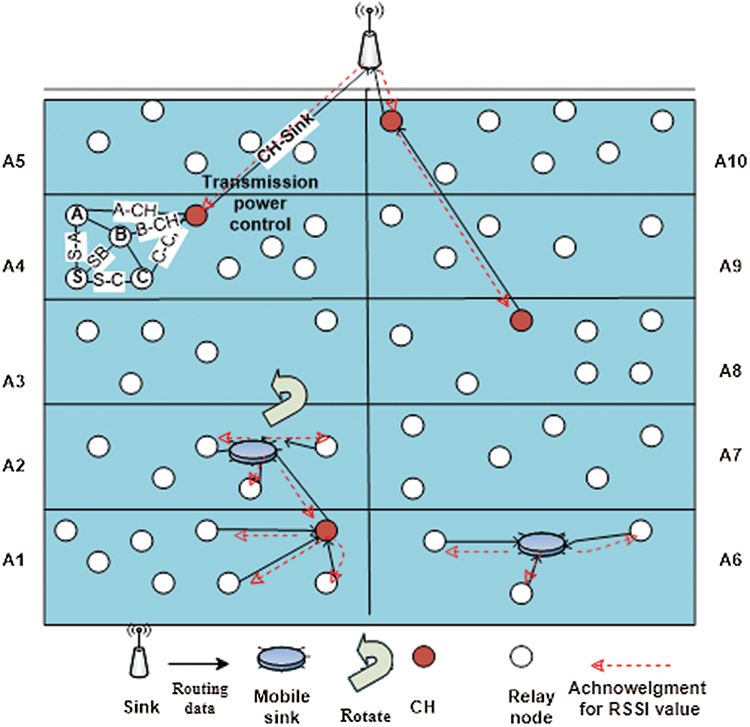
Figure 3: System model
We divide the site into 10 sub-areas of equal size to specify the dense and sparse areas. AE and AW refer to the right and left side areas, respectively. The start point coordinates considered a measure point for area creation. Start point coordinates are referred to as S(X0; Y0).
The following equations split the network site into five left side areas:
The following equations split the network site into five right side areas:
where B is the X-axis point of an area. Double B is used for the right side areas of AE, and B is used for AW’s left side areas. B’s value is estimated from a total breadth of the network site.
Eq. (14) calculates the value of B.
where L is calculated from the length of the network site. L is the Y-axis point of an area. The values of AW1 and AE1 are L. Double L for AW2 and AE2, multiple of 3 for AW3 and AE3, multiple of 4 for AW4 and AE4 and multiple of 5 for AW5 and AE5.
From Eqs. (16) and (17), we built a relation to find point L for AWn and AEn as:
where N is the number of areas located either left or right. The coordinates for an Nth number of the top left area AWn and top right region AEn can be calculated as:
4.2 Searching Sparse and Dense Area Algorithms
Sparse and dense regions are determined through Algorithms 1 and 2, as mentioned by the SEEC protocol, respectively [7]. In both algorithms, node N coordinates searched it and then searched for other nodes in the surrounding. Considering that the network is divided into S small sections if n is part of this particular small section, then this region is sparse. Otherwise, it will be dense. The whole mechanism of finding sparse and dense areas is shown in Fig. 4.
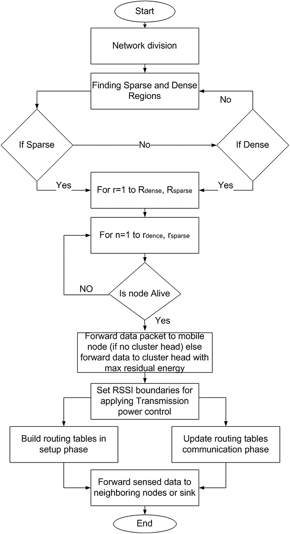
Figure 4: CTP-SEEC implementation flowchart
4.3 Clustering and CH Selection in Dense Area
When sparse and dense areas are sought, the following stage is a grouping of nodes in dense areas. We utilized a grouping strategy for areas with the highest density to expend energy productivity and system lifespan. In SEEC, the nodes in a dense area cooperatively selects a node to be the CH and then transmit information to the elected CH. The head performs information conglomeration and transmits the compacted information to any of the closest sinks. The choice of the CH is determined by the bottom and remaining energy. CH selection: The process of determining CH in SEEC is not the same as those in different protocols. In SEEC, a node with low bottom and remaining high power is selected as a CH. The choice model of selecting a node as a CH in a particular area depends on the accompanying conditions:
where
where,
where Ab is the profundity of nodes of an area, most importantly. For the choice of CH, Condition (21) is checked. On the off chance that the bottom of the node is higher than the alternate nodes of that area, the node at that point cannot be a CH in the current round, and if the bottom of the node is lower than the alternate nodes of that particular area at that point, then Condition (22) is checked, where PCH is the excess power of a CH, and Pm is the mean leftover power of an individual node. The node is chosen as a CH if the its remaining power is more prominent than the normal remaining power determined for an individual node. In Condition (23), C is the chance of a node to be a CH. C is determined toward the beginning of each tour, and t speaks to the current round. The node is chosen as the bunch head when it has not been CH for the last 1 = c tours. The node produces an irregular number rand, which contrasts the rand esteem and Th (i). The node is considered an ordinary node if the rand of a node is more noteworthy than the threshold. When the rand of the node is not as much as Th threshold, the node at that point is finally a CH node. In SEEC [7], only a single node is chosen as a CH in each thick area per tour. We show a case of sensor node choice as a CH. In Fig. 5A, two nodes, namely, N1 and N2, have different energy levels at similar depths. The node with high remaining energy is chosen as a CH (i.e., N2), whereas in Fig. 5B, the node N1 is chosen as a CH. Both nodes have the same energy level, yet they have various depths. Along these lines, the low depth node is chosen as a CH.
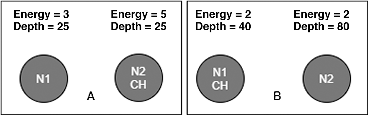
Figure 5: CH selection [7]
In this phase of network arrangement, its field is distributed into n sections, and relay nodes are arbitrarily positioned in the network area (Fig. 3). Considering that a single static sink and architecture are used, one fixed sink exists at the surface area. By contrast, MSs are positioned inside the sparse region. The static sink node advertises a ping message (control packet) across the dense regions of the network. A ping message with a cost value and zero is originated from the static sink node. Receiving CH nodes adjacent to the sink receive the ping message and update its distance from the sink in the form of the number of hops from the sink fixed at the surface.
Moreover, each receiving node sets a suitable transmission power level (TPL) with the sink based on the received signal strength indicator (RSSI). The cost values in the number of hops are forwarded after a delay1 to other CH in the adjustment dense regions. The receiving CH nodes store the cost value and set a suitable TPL based on RSSI. Each node determines its distance from the sink along these lines, sets a suitable TPL, and then broadcasts this information in its transmission range. Other nodes follow the same procedure. If a node receives a value greater than its current one, then it disposes the ping message; otherwise, it refreshes its distance information, sets a suitable TPL, and broadcasts the ping message again to nodes in its transmission range. This procedure continues until each sensor node sets a suitable TPL with the selected neighbors and obtains its distance from the sink. In brief, the control packet in the form of a ping message contains a cost field, which reflects the number of hops to reach the sink. In the setup phase, such control packets are propagated throughout the network. This approach establishes a minimum or shortest route from source to sink and achieves the TPL adjustment of each node with its selected neighboring nodes.
4.5 Sink Mobility in Sparse Area
Sparse regions refer to the areas with the least number of nodes. Sparse regions are sought, and two portable sinks are located in these regions for information gathering in SEEC. The sinks are versatile. For instance, moving sink 1 (MS1) varies its situation every round from highest in sparsity to lowest meagre sparsity aside from the district of MS2. However, MS2 stays in the area with the highest sparsity until every sensor node in the region passes. All sensor nodes are kicked by MS2. At that point, it converts its situation into the area with the highest sparsity among the remaining sparse areas.
Meanwhile, MS1 varies its location as required. The MSs should be placed around the center of the region so that most of the nodes connect with it. Sparsity is the most reasonable way to deal with gathering information from the greatest sensor nodes of the system, to accomplish something great using the least energy of the whole system. Likewise, awareness of the sparsity approach is useful in discovering the dense areas of the system field, where the sensor hubs structure groups. Instead, the sensor hubs transmit information to the sinks through multi bouncing, and nodes transmit information to their district’s particular CH. In this manner, only the CH sends information to the sink. Due to these instances, SEEC is considered an energy effective protocol.
After splitting the site of the network into subareas logically (Fig. 3) for identification, the network site is established to limit the sink’s movement in the sparse area only. Moreover, dense and sparse areas are estimated to begin data transmission in the network. Therefore, two algorithms are suggested:
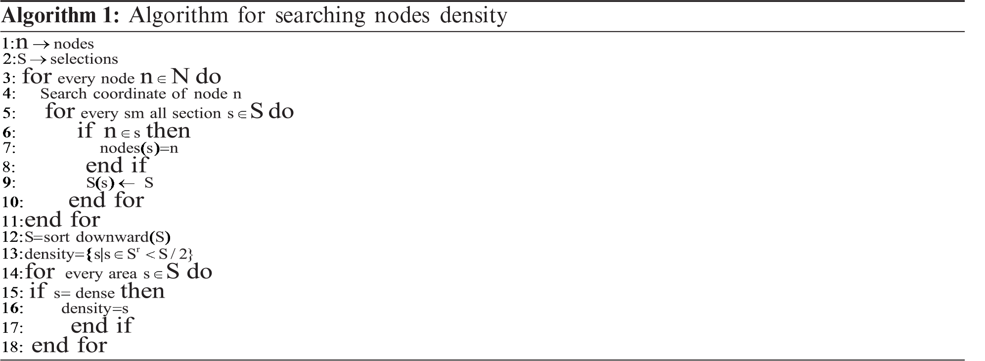
Algorithm 1 or DSA is used to find dense regions in the network. Algorithm 2 or SSA is used to find sparse regions. These algorithms search for the number of sensor nodes in each zone. The zones are sorted in ascending array based on the number of nodes. Based on the nodes’ density in each logical area, the sparse and dense areas are specified. For example, [5] is assumed to be selected as a dense area. Thus, the Nth number of nodes should be available to satisfy the limited threshold by using the following equation. The area is dense when N is greater or equal to the Nth, and the opposite indicates a sparse area. The sparse and dense search approaches are used in Fig. 3 to estimate the network’s sparse and dense areas, respectively. Afterwards, the two MSs are deployed in the network’s sparse area; MS1 is placed at a maximum sparse area, and MS2 at a minimum sparse area (Fig. 3).
Both of them move from maximum sparse to the minimum sparse area and change their regions after each round from most sparse to the least sparse region and the opposite correct. In this way, more areas are covered with a void energy hole creation. As a result, more PDR would be achieved. In a dense area, the clustering approach is used. CH is selected using the procedure discussed earlier. A CH node refers to a node with high remaining energy and low depth (Fig. 5).
The MS nodes move in the sparse regions with very few nodes. The first MS moves within such regions while the second MS remains in such a region until all the nodes die.
When cost fields are built up through the network in the setup phase, a node that wants to direct information to the sink uses the minimum cost path. The node directs the information bundle to its minimum cost adjoining node while its adjusted TPL is stored in the routing table. After the reception of data packets, the sender node (source or relay) acknowledges the receiving node and the RSSI value. Suppose the RSSI crosses its predefined limit specified as either low or high. In that case, the sender node tunes its TPL accordingly, that is, it switches to the next power level if RSSI is below the limit. By contrast, if the RSSI is above the high limit, the power level declines to a level. The RSSI limits are fixed at the beginning of the data communication phase, depending on the channel condition. The proposed technique is depicted in Fig. 3, where n is the number of nodes, and R is the region.

This section presents a simulation setup and parameter to evaluate the performance of our proposed protocol (CTPSEEC) in terms of network lifetime, stability period, residual energy, packets received per round, and total packets received at the sink. The simulation period consists of 3500 rounds to obtain accurate results using the same environmental parameters. The total number of 100 sensor nodes is deployed randomly in 100 m × 100 m underwater. Initially, each node contains 5 joules of energy. Each sensor node can transmit in the range of 50 m. The depth threshold is set to 15 m. The proposed protocol is evaluated on the basis of the following metrics:
This metric shows how much time the network nodes function. It refers to the total number of rounds when all network field nodes are alive and functional. This metric is important when considering the effectiveness of a scheme because energy is the primary concern in UWSNs. The ultimate purpose of most of the underwater environment mechanisms is to extend the network lifetime, which is dependent on energy consumption.
5.2 Packets Received per Round
This analysis demonstrates the ratio of packets received at the sink in the particular round and their capability to accept the data packets. If the sending packets’ ratio exceeds the threshold, then the packet will be dropped.
This metric refers to the variance concerning each node’s initial energy and total energy after the transmission and reception of data packets.
6 Simulation Results and Discussion
This section presents the performance evaluation of the proposed scheme in terms of network lifetime, stability period, residual energy, packets received per round, and total packets received at the sink. To verify the proposed scheme, rigorous comparison with current state-of-the-art schemes is conducted. For this purpose, we have considered the DBR [9], EEDBR [24], and SEEC [7] underwater routing schemes.
The network lifetime is improved after implementing the controlled transmission strategy in SEEC (Fig. 6). In SEEC, each sensor node transmitted packets at a predefined transmission power, thereby causing the network to die early. In the controlled transmission power (CTP) strategy, the source node based on Euclidean distance to the destination node adjusts transmission power. These power adjustments have varying energy consumption every time the packet is sent. This variation in energy consumption boosts the network’s lifetime.
Fig. 6 shows that the nodes in SEEC with CTP are alive at round 3500, whereas the SEEC without CTP is dead at round 2500 (Fig. 7). During the information sending in DBR, the sender incorporates its depth, and the data packets that accept nodes contrast their depths with the sender node. The node with a small depth advances packet to the sink. Every node possesses a specific holding time for every data packet. Thus, nodes with smaller depths have shorter holding time. Considering that only the sensor node’s depth is utilized for sending, these nodes die prior to alternate nodes, thereby resulting in energy holes. Fig. 6 shows that the nodes in DBR with CTP are alive at round 3500, whereas those without CTP are dead at round 2000 (Fig. 7). In EEDBR, the stability period is better than that in DBR (Fig. 6). Neighbors of the nodes rapidly reduce, thereby causing network instability, and the load on nodes is higher in EEDBR when the network is sparse. Hence, the number of dead nodes increases abruptly (Fig. 7).
Fig. 6 shows that the nodes in EEDBR with CTP are alive at round 3500, whereas the EEDBR without CTP is dead at round 2000 (Fig. 7).
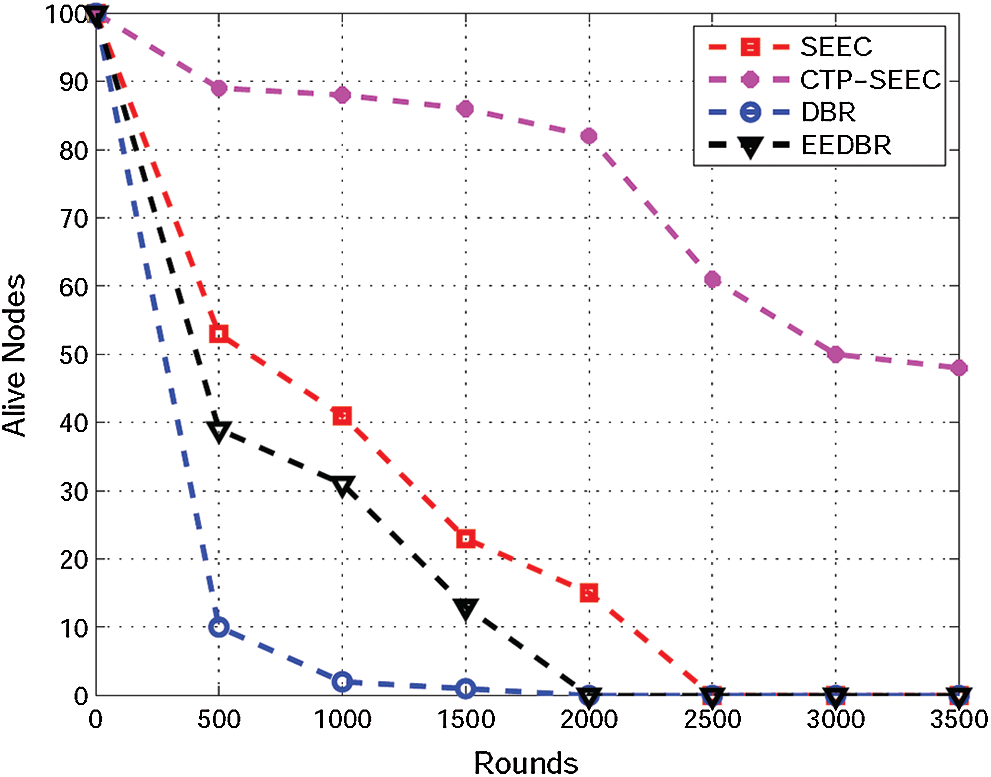
Figure 6: Alive nodes
The random deployment of sensor nodes does not always provide the same number of dense and sparse regions. Suppose the number of dense regions is maximum. The nodes within the same dense regions communicate with the same transmission power. In that case, the stability period is compromised.
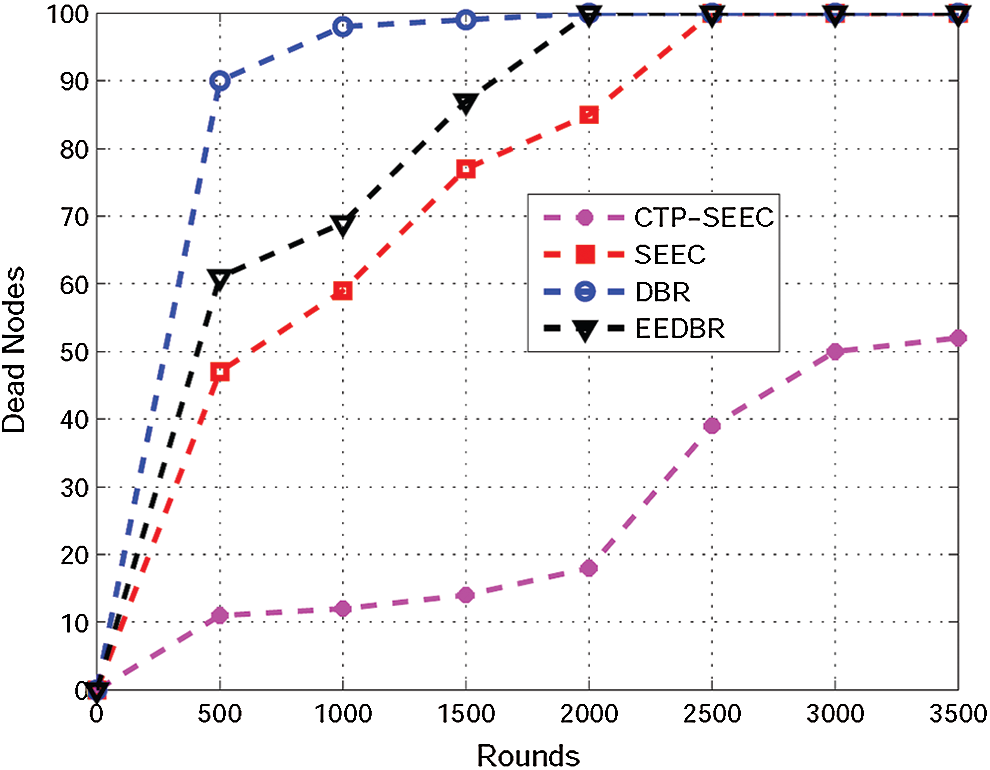
Figure 7: Dead nodes
Furthermore, a controlled transmission power strategy can be adapted, and then the stability period is improved (Fig. 7). In the CTP-SEEC, clustering used in dense areas and MS nodes in sparse areas increase the stability period better than SEEC, DBR, and EEDBR. In DBR, the greedy mechanism forces the rigid election of transmitter node based on which the nodes are assigned.
Thus, resources continue to be underutilized, thereby causing the lowest stability period for the protocol. The nodes in DBR without CTP are dead at round 2000 (Fig. 7). In EEDBR, nodes begin to die quickly because of excessive data forwarding and rapid energy reduction.
6.3 Packets Received per Round
Fig. 8 reveals that the total packets collected in CTP-SEEC at the sink are high. This phenomenon is due to the increase in network lifetime that resulted from the use of the controlled transmission power strategy. In addition, a high number of alive nodes throughout the network lifetime improved PDR for CTPSEEC. Packets received per round in EEDBR result in high residual energy, whereas only selecting nodes by considering residual energy cannot achieve a high PDR in the sparse region. In DBR, only the lower depth of the nodes are considered for transmitting the packets, thereby resulting in the duplication of packets that causes the lowest DBR among all the other protocols. In the SEEC protocol, the number of packets collected at the sink node is lesser than the suggested CTP-SSEC routing protocol. The reason behind this is that, in SEEC, the transmission power remains constant, and the network dies early.
In SEEC, the factor of transmission power in the equation was constant. Regardless of the distance between two communicating nodes, almost the same amount of energy was consumed while transmitting a packet. In CTP-SEEC, the function varies its return value after sending the packet, thereby resulting in tremendous residual energy. In the proposed scheme, transmission power is adjusted on the basis of the range from the source to the destination node. The lesser the distance, the lesser the transmission power and vice versa. Less transmission power results in less energy tax, thereby resulting in higher network residual energy in CTP-SEEC. DBR only considers depth and fails to consider the residual energy. Thus, it has the minimum residual energy.
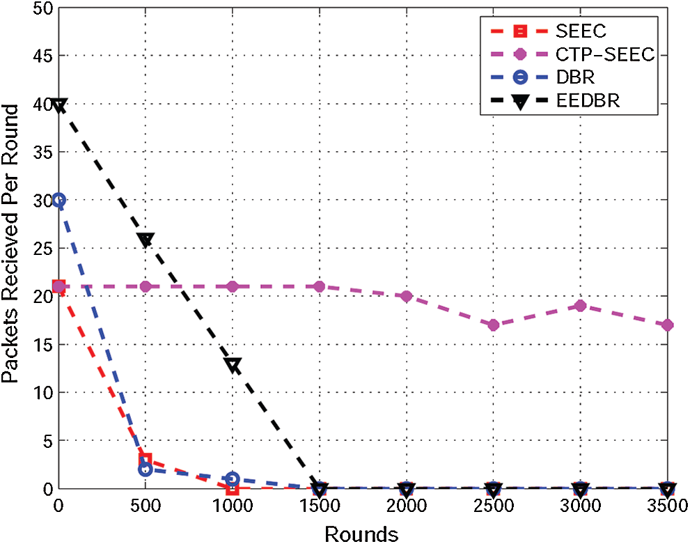
Figure 8: Packets received per round
In EEDBR, selecting nodes by only considering residual energy cannot achieve a high PDR in the sparse region. The total remaining energy depletion of CTP-SEEC, SEEC, EEDBR, and DBR is illustrated in Fig. 9.
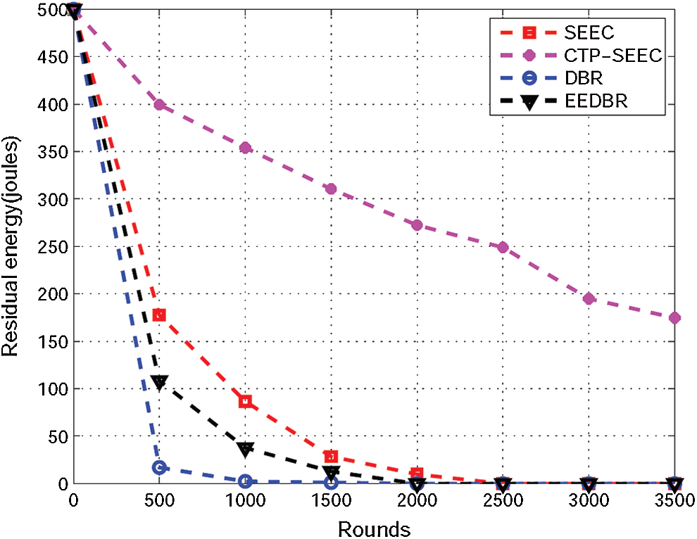
Figure 9: Residual energy
This article investigated the existing methods of different energy-efficient location-free routing protocols of UWSN. Existing studies do not address multiple issues, including the failure to adjust sensor nodes’ transmission power during data transmission. Moreover, existing strategies utilize one or more static sinks at the water’s surface using different routing mechanisms during data transmission from source to sink. This phenomenon creates a scalability issue when the network size increases (e.g., bottleneck creation) and reduces network performance. These problems result in rapid energy depletion with a low PDR. Thus, the overall network lifetime is reduced. Therefore, we proposed a new protocol with a balanced energy-saving technique and developed an energy-efficient strategy to lengthen the overall network lifetime. Simulation analysis is applied to analyze the recommended strategies’ execution by contrasting it with DBR, EEDBR, and SEEC routing protocols. In addition to revealing that our proposed protocol outperforms the best existing state-of-the-art, such as DBR, EEDBR, and SEEC routing protocols, in terms of network lifetime and PDR, the simulation results proved the effectiveness of our proposed protocol. In the future, we will explore the monitoring of the sparsity networks by avoiding the energy hole creation problem. The proposed scheme has addressed this problem to some extent. However, the smart and adaptive mobility mechanism of MSs can also influence the avoidance of energy hole creation significantly. Although not required, MSs with CTP result in end-to-end delays. Thus, the delay in each round is still observed. The proposed scheme should be modified to address these problems in future work.
Funding Statement: The authors are grateful to the Deanship of Scientific Research and King Saud University for funding this research. The author are also grateful to Taif University Researchers Supporting Project number (TURSP-2020/215), Taif University, Taif, Saudi Arabia. This research work was also partially supported by the Faculty of Computer Science and Information Technology, University of Malaya under Postgraduate Research Grant (PG035-2016A).
Conflicts of Interest: The authors declare that they have no conflicts of interest to report regarding the present study.
1. L. Parra, S. Sendra, L. García and J. Lloret, “Design and deployment of low-cost sensors for monitoring the water quality and fish behavior in aquaculture tanks during the feeding process,” Sensors, vol. 18, no. 3, pp. 750, 2018. [Google Scholar]
2. R. W. Coutinho, A. Boukerche, L. F. Vieira and A. A. Loureiro, “Geographic and opportunistic routing for underwater sensor networks,” IEEE Transactions on Computers, vol. 65, no. 2, pp. 548–561, 2015. [Google Scholar]
3. S. Sendra, J. Lloret, J. M. Jimenez and L. Parra, “Underwater acoustic modems,” IEEE Sensors Journal, vol. 16, no. 11, pp. 4063–4071, 2015. [Google Scholar]
4. H. Yu, N. Yao and J. Liu, “An adaptive routing protocol in underwater sparse acoustic sensor networks,” Ad Hoc Networks, vol. 34, pp. 121–143, 2015. [Google Scholar]
5. A. Sher, N. Javaid, I. Azam, H. Ahmad, W. Abdul et al., “Monitoring square and circular fields with sensors using energy-efficient cluster-based routing for underwater wireless sensor networks,” International Journal of Distributed Sensor Networks, vol. 13, no. 7, pp. 1550147717717189, 2017. [Google Scholar]
6. G. Ahmed and N. M. Khan, “Adaptive power-control based energy-efficient routing in wireless sensor networks,” Wireless Personal Communications, vol. 94, no. 3, pp. 1297–1329, 2017. [Google Scholar]
7. I. Azam, A. Majid, I. Ahmad, U. Shakeel, H. Maqsood et al., “SEEC: Sparsity-aware energy efficient clustering protocol for underwater wireless sensor networks,” in IEEE 30th Int. Conf. on Advanced Information Networking and Applications, Crans-Montana, Switzerland, pp. 352–361, 2016. [Google Scholar]
8. A. Sher, A. Khan, N. Javaid, S. H. Ahmed, M. Y. Aalsalem et al., “Void hole avoidance for reliable data delivery in IoT enabled underwater wireless sensor networks,” Sensors, vol. 18, no. 10, pp. 3271, 2018. [Google Scholar]
9. H. Yan, Z. J. Shi and J.-H. Cui, DBR: Depth-Based Routing for Underwater Sensor Networks, Springer, Berlin, Heidelberg: Springer, pp. 72–86, 2008. [Google Scholar]
10. A. Yahya, S. U. Islam, A. Akhunzada, G. Ahmed, S. Shamshirband et al., “Towards efficient sink mobility in underwater wireless sensor networks,” Energies, vol. 11, no. 6, pp. 1471, 2018. [Google Scholar]
11. S. Shah, A. Khan, I. Ali, K.-M. Ko and H. Mahmood, “Localization free energy efficient and cooperative routing protocols for underwater wireless sensor networks,” Symmetry, vol. 10, no. 10, pp. 498, 2018. [Google Scholar]
12. S. N. Pari, M. Sathish and K. Arumugam, “An energy-efficient and reliable depth-based routing protocol for underwater wireless sensor network (ER-DBR),” in Advances in Power Systems and Energy Management, Springer, pp. 451–463, 2018. [Google Scholar]
13. L. Kong, K. Ma, B. Qiao and X. Guo, “Adaptive relay chain routing with load balancing and high energy efficiency,” IEEE Sensors Journal, vol. 16, no. 14, pp. 5826–5836, 2016. [Google Scholar]
14. Z. Zhou, B. Yao, R. Xing, L. Shu and S. Bu, “E-CARP: An energy efficient routing protocol for UWSNs in the internet of underwater things,” IEEE Sensors Journal, vol. 16, no. 11, pp. 4072–4082, 2015. [Google Scholar]
15. Y. Noh, U. Lee, S. Lee, P. Wang, L. F. Vieira et al., “Hydrocast: Pressure routing for underwater sensor networks,” IEEE Transactions on Vehicular Technology, vol. 65, no. 1, pp. 333–347, 2015. [Google Scholar]
16. J. So and H. Byun, “Load-balanced opportunistic routing for duty-cycled wireless sensor networks,” IEEE Transactions on Mobile Computing, vol. 16, no. 7, pp. 1940–1955, 2016. [Google Scholar]
17. M. Z. Abbas, K. A. Bakar, M. Ayaz, M. H. Mohamed, M. Tariq et al., “Hop-by-hop dynamic addressing based routing protocol for monitoring of long range underwater pipeline,” KSII Transactions on Internet, vol. 11, no. 2, pp. 731–763, 2017. [Google Scholar]
18. S. Yu, S. Liu and P. Jiang, “A high-efficiency uneven cluster deployment algorithm based on network layered for event coverage in UWSNs,” Sensors, vol. 16, no. 12, pp. 2103, 2016. [Google Scholar]
19. A. Khan, I. Ali, A. U. Rahman, M. Imran and H. Mahmood, “Co-EEORS: Cooperative energy efficient optimal relay selection protocol for underwater wireless sensor networks,” IEEE Access, vol. 6, pp. 28777–28789, 2018. [Google Scholar]
20. S. Yadav and V. Kumar, “Optimal clustering in underwater wireless sensor networks: Acoustic, EM and FSO communication compliant technique,” IEEE Access, vol. 5, pp. 12761–12776, 2017. [Google Scholar]
21. V. Sasikala and C. Chandrasekar, “Cluster based sleep/wakeup scheduling technique for WSN,” International Journal of Computer Applications, vol. 72, no. 8, pp. 15–20, 2013. [Google Scholar]
22. P. S. Rao, P. K. Jana and H. Banka, “A particle swarm optimization based energy efficient cluster head selection algorithm for wireless sensor networks,” Wireless Networks, vol. 23, no. 7, pp. 2005–2020, 2017. [Google Scholar]
23. I. Ez-Zazi, M. Arioua, A. El Oualkadi and P. Lorenz, “On the performance of adaptive coding schemes for energy efficient and reliable clustered wireless sensor networks,” Ad Hoc Networks, vol. 64, pp. 99–111, 2017. [Google Scholar]
24. S. Mahmood, H. Nasir, S. Tariq, H. Ashraf, M. Pervaiz et al., “Forwarding nodes constraint based DBR (CDBR) and EEDBR (CEEDBR) in underwater WSNs,” Procedia Computer Science, vol. 34, pp. 228–235, 2014. [Google Scholar]
25. J. Luo, Y. Chen, M. Wu and Y. Yang, “A survey of routing protocols for underwater wireless sensor networks,” IEEE Communications Surveys, vol. 23, pp. 137–160, 2021. [Google Scholar]
26. X. Xiao, H. Huang and W. Wang, “Underwater wireless sensor networks: An energy-efficient clustering routing protocol based on data fusion and genetic algorithms,” Applied Sciences, vol. 11, no. 1, pp. 312, 2021. [Google Scholar]
27. X. Su, I. Ullah, X. Liu and D. Choi, “A review of underwater localization techniques, algorithms, and challenges,” Journal of Sensors, vol. 2020, pp. 1–24, 2020. [Google Scholar]
 | This work is licensed under a Creative Commons Attribution 4.0 International License, which permits unrestricted use, distribution, and reproduction in any medium, provided the original work is properly cited. |