Computers, Materials & Continua DOI:10.32604/cmc.2021.017300
Article

Guided Intra-Patch Smoothing Graph Filtering for Single-Image Denoising

Yibin Tang1, Ying Chen2, Aimin Jiang1, Jian Li1, Yan Zhou*,1 and Hon Keung Kwan3

1College of Internet of Things Engineering, Hohai University, Changzhou, 213022, China
2School of Microelectronics and Control Engineering, Changzhou University, Changzhou, 213022, China
3Department of Electrical Engineering, University of Windsor, Ontario, N9B 3P4, Canada
*Corresponding Author: Yan Zhou. Email: yanzhou@hhu.edu.cn
Received: 26 January 2021; Accepted: 04 March 2021

Abstract: Graph filtering is an important part of graph signal processing and a useful tool for image denoising. Existing graph filtering methods, such as adaptive weighted graph filtering (AWGF), focus on coefficient shrinkage strategies in a graph-frequency domain. However, they seldom consider the image attributes in their graph-filtering procedure. Consequently, the denoising performance of graph filtering is barely comparable with that of other state-of-the-art denoising methods. To fully exploit the image attributes, we propose a guided intra-patch smoothing AWGF (AWGF-GPS) method for single-image denoising. Unlike AWGF, which employs graph topology on patches, AWGF-GPS learns the topology of superpixels by introducing the pixel smoothing attribute of a patch. This operation forces the restored pixels to smoothly evolve in local areas, where both intra- and inter-patch relationships of the image are utilized during patch restoration. Meanwhile, a guided-patch regularizer is incorporated into AWGF-GPS. The guided patch is obtained in advance using a maximum-a-posteriori probability estimator. Because the guided patch is considered as a sketch of a denoised patch, AWGF-GPS can effectively supervise patch restoration during graph filtering to increase the reliability of the denoised patch. Experiments demonstrate that the AWGF-GPS method suitably rebuilds denoising images. It outperforms most state-of-the-art single-image denoising methods and is competitive with certain deep-learning methods. In particular, it has the advantage of managing images with significant noise.

Keywords: Graph filtering; image denoising; MAP estimation; superpixel

1  Introduction

Image denoising aims to remove noise from images, thereby benefitting the subsequent analysis and processing of images and videos. Current image denoising methods are divided into two categories: Model- and deep-learning-based methods. Prior to the success of deep learning methods, model-based methods have been used for decades to exploit the intrinsic attributes of images [1–3]. Most of them resolve the denoising problem using the internal prior of the target noisy image without considering other images. Therefore, they are often considered as single-image denoising methods. In contrast, deep-learning-based methods employ the external prior from other image databases to recover denoised images. Thus, they can be considered as data-driven methods that require numerous image data [4–6]. Flexible feature learning strategies are adopted in these methods via various deep networks. Because of the feature analysis of external images instead of the target image, deep-learning-based methods have a higher denoising performance than the model-based methods. However, in this study, we focus on the model-based denoising method assuming that only a single noisy image is provided.

In general, model-based denoising methods involve a filtering process, where the input and output data are noisy and denoised images, respectively. Thus, various filtering methods are used in different domains such as spatial, transform, and learned domains. In earlier studies, spatial-domain methods, such as bilateral filtering [7] and non-local means filtering [8], were used for the direct operation on pixels or patches. A spatial smoothing filter was used to remove noise-like components from the target image. However, since this smoothing procedure is only performed in local areas or patch groups, spatial filtering has a limited ability to exploit the statistical information of the entire image. To overcome this problem, transform-domain filters are presented by considering the directional structures in the images. Wavelet and Curvelet filters have been successfully employed for their adequate structural description of basis [9–11]. A popular denoising method, named block matching and three-dimensional (BM3D) filtering, was proposed using a collaborative spatial-wavelet filter [12,13]. It adopts a spatial filtering result to guide sequential wavelet filtering on similar patches. Unfortunately, none of the aforementioned filters are contented-based due to their fixed filter coefficients. Therefore, more advanced models, such as sparse representation and low-rank representation models [3,14–16], have been deployed in different learned domains in recent years. For example, a trilateral weighted sparse coding (TWSC) method is used to estimate data fidelity based on the sparse representation theory [17]. A low-rank approximation approach with adaptive regularizer learning (ARLLR) [18] is presented to shrink the eigenvalues of patches and is highly successful in image denoising. However, it is not yet considered as a filter-based model. The current study proves that the low-rank model is equivalent to a subspace graph filter [19]. The filtering procedure takes place in a graph subspace supported by the eigenvectors of the patch group.

Graph filtering is an essential component of graph signal processing. Its basic idea is to filter the input signal on the network nodes [20]. Once pixels or patches are chosen according to the nodes, graph filtering can adequately fit image denoising. Certain graph polynomial filtering methods are presented to employ various Laplacian matrix regularizers in the existing denoising model [21–23]. Several adaptive graph filtering methods are also proposed, by applying different coefficient shrinkage strategies in the graph-frequency domain. In a pioneer work, an idea lowpass graph filter was designed using a full shrinkage approach in the high graph-frequency band, achieving denoising performance comparable with that of BM3D [24–26]. Given a patch group, the study proves that the eigenvectors of the Laplacian matrix are a set of graph Fourier bases [27]. Recently, an adaptive weighted graph filtering (AWGF) method introduced an effective shrinkage approach in the entire band [19]. Although it theoretically builds a bridge from the existing low-rank model to graph filtering, its denoising performance is barely comparable with that of low-rank denoising methods. In the traditional AWGF method, the graph filter is prioritized, whereas patch attributes are seldom considered for image denoising.

Motivated by the recent progress, we propose a guided intra-patch smoothing AWGF (AWGF-GPS) method for single-image denoising. Our contributions are twofold. (1) Unlike AWGF that uses graph topology on patches, AWGF-GPS learns the superpixel graph to exploit the pixel smoothing attribute in patches. This operation forces the restored pixels to smoothly evolve in the local area, where both intra- and inter-patch relationships are utilized during patch restoration. (2) A guided-patch regularizer is incorporated into AWGF-GPS. The guided patch is obtained in advance using a maximum-a-posteriori (MAP) probability estimator. By considering the guided patch as a sketch of a denoised patch, AWGF-GPS effectively supervises the patch restoration procedure. Consequently, the reliability of the denoised patch is increased. Experiments demonstrate that our AWGF-GPS method suitably rebuilds denoising images. It outperforms most state-of-the-art model-based methods and is competitive with certain deep-learning methods.

2  Related Work

We briefly review the existing AWGF model [19]. Given a noisy patch group, Y, with vectorized patches {yi} in its column, the AWGF model is expressed as

{σ̃g,i}= argmin{σg,i}12τ∥Y-YUgΣgUgT∥F2+∑i=1Ng(σg,i),(1)

where τ is a weighted coefficient, Ug is a graph Fourier basis matrix of the graph filter, N is the patch number, and Σg is a diagonal matrix with the shrinkage coefficients {σg,i} as its diagonal entries. Moreover, g(σg,i) is a prior regularizer, where different regularizers can be adopted to generate various shrinkage strategies on σg,i [28,29]. Sequentially, the denoised patch group, X, is obtained as

X=YUgΣ̃gUgT,(2)

where Σ̃g is a diagonal matrix with the optimal shrinkage coefficients {σ̃g,i} as its diagonal entries.

Note that the noisy patch group, Y, in Eq. (2) is right-multiplied by the filtering operation of UgΣ̃gUgT. Because the graph filter is built on the graph topology constructed among patch nodes, the AWGF model is an intrinsic patch-based graph filtering model. It focuses on the relationship between patches, where the similarity attribute of the pixels is not considered.

3  Proposed Method

We propose the AWGF-GPS method to employ both the self-similarity of patches and the local similarity of intra-patch pixels. Fig. 1 depicts the filtering flowchart. The superpixel is defined as a pixel set sharing the same location on the patches. A graph is learned using these superpixels to strengthen the smooth attributes of the neighboring pixels. Sequentially, the corresponding graph Fourier bases are obtained from the Laplacian matrix during the graph analysis. The guided patches are evaluated based on their corresponding noisy patches via a MAP estimator. Combined with the graph Fourier bases and the guided patches, the AWGF-GPS model is finally implemented to restore the denoised patches.

3.1 Graph Learning on Superpixels

We obtain the superpixels from the noisy patch group, Y, where each row vector of Y represents a superpixel node. Graph learning is then performed on these nodes. Various graph learning methods have been proposed to form graphs with different strategies. However, we prefer a log-model graph learning approach [30], which builds a connected graph without any isolated nodes. This graph learning model is described as

W̃= argminW∥Z∘W∥1-α1T logW1+β∥W∥F2,(3)

where W is an adjacent matrix to measure the weighted edges among the superpixel nodes, Z is a pairwise distance matrix for the superpixels, α and β are two weighted coefficients, 1 represents a vector of ones, and symbol ∘ denotes the Hadamard product.

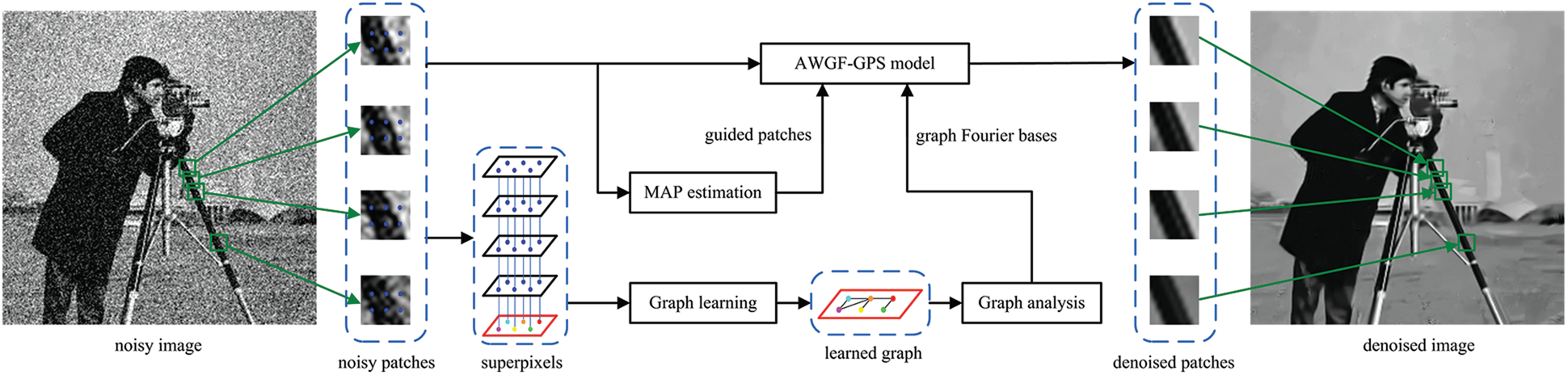
Figure 1: Flowchart of AWGF-GPS denoising

The optimization problem in Eq. (3) can be conveniently solved using the GSP Toolbox [31]. Then, the graph Laplacian matrix is given as L=D-W, where the diagonal entry of the degree matrix, D, is the corresponding row sum of W. Finally, the graph Fourier bases, Ug, are obtained from the eigenvectors of L.

3.2 Guided Patch Estimation

We employ the guided patches as a regularizer in our AWGF-GPS model. Here, a MAP estimator is used to generate the guided patch group, X^, that is viewed as a sketch of the denoised patch group, X. For convenience, we interpret the MAP estimator at the pixel level [32] and then extend it to the patch operation level. Given a noisy pixel, y = x + n, with clean pixel x and noise n, where n follows a Gaussian distribution, N(0,σn2), with a zero mean value and standard deviation σn, the conditional probability of x can be expressed as

p(x∣y)=12πσ^x 2 exp{-(x-μ^)22σ^x2}.(4)

In Eq. (4), symbols μ^ and σ^x2 are respectively defined as

μ^=σn2x̄+σx2yσn2+σx2,(5)

σ^x2=σn2σx2σn2+σx2,(6)

where x̄ and σx are the mean value and standard deviation of x, respectively. Hence, we define the guided pixel, x^, as the conditional expected value of x with

x^=∫-∞∞x⋅p(x∣y)dx=x̄1+S+y1+1/S,(7)

where S=σx2/σn2 is the signal-to-noise ratio (SNR). Inspired by the pixel estimation of x^, the guided group, X^, can be written as

X^=X̄1+S+Y1+1/S,(8)

where X̄ is the mean patch group composed of the corresponding guided pixels. In Eq. (8), we assume that each pixel in the patch group shares the same SNR.

Unfortunately, the guided group, X^, in Eq. (8) is impractical because there is no exquisite formulation for X̄ and S. As a result, we generate these two parameters by an alternative approach. To estimate the SNR, we approximate S as

S≈var(Y)-σn2σn2,(9)

where var(Y) is the mean deviation of pixel for patch group Y.

We estimate the mean patch group, X̄, using an ideal lowpass graph filter as

X̄≈UgΣ̃g,MUgTY,(10)

where the diagonal matrix, Σ̃g,M, contains only the first M nonzero diagonal entries. These entries are described as

σg,i={1i≤M0otherwise.(11)

The optimal value of M is further achieved under the noise control of σn2 as

M̃= argminM|var(UgΣg,MUgTY)+σn2-var(Y)|.(12)

3.3 AWGF-GPS Model

Using graph Fourier bases and guided patches, we define the AWGF-GPS model as

{σ̃g,i}= argmin{σg,i}12τ∥Y-UgΣgUgTY∥F2+∑i=1N′g(σg,i)+γ∥X^-UgΣgUgTY∥F2,(13)

where γ is a weighted coefficient and N′ is the superpixel number. Then the denoised patch group, X, is obtained as

X=UgΣ̃gUgTY.(14)

We should mention some aspects of the filtering procedure from Eqs. (13) to (14). Unlike the definition in Eq. (2), the noisy patch group, Y, in Eq. (14) is left-multiplied by the filtering operation of UgΣ̃gUgT. In this case, the row combination process is employed for Y. Since each row vector of Y represents a superpixel, it conducts a superpixel-based filtering model. Moreover, we aim for the denoising patches described in Eq. (13) to be centralized with X^, because the guided patch group, X^, is another denoised result for clean patches. These guide patches provide an optimal direction for denoising.

To simplify Eq. (13), we transform the model by merging its first and third terms as

{σ̃g,i}= argmin{σg,i}(1+2λτ)∥UgΣgUgTY-11+2λτ(Y+2λτX^)∥F2+2τ∑i=1N′g(σg,i).(15)

Subsequently, we cast Eq. (15) in the trace form as

{σ̃g,i}= argmin{σg,i}(1+2λτ)trace(Σg2UgTYYTUg-2ΣgUgTYETUg)+2λτ∑i=1N′g(σg,i),(16)

where E=(1+2λτ)-1(Y+2λτX^).

Then, we provide the setting of the prior regularizer, g(σg,i). According to the AWGF approach [19], regularizer g(σg,i) is expressed as

g(σg,i)= log|ηiσg,i+ε|,(17)

where ε is a small positive constant and ηi is a weighted coefficient. By defining the projection matrix, P=YTUg, with its vectors {pi}, we set ηi as the projected energy with ηi2=piTpi.

Because the shrinkage coefficient matrix, Σg, is diagonal, the optimization problem in Eq. (16) can be decomposed into a set of subproblems by the given g(σg,i) of Eq. (17). For each shrinkage coefficient, σg,i, the corresponding subproblem is written as

σ̃g,i= argminσg,i(1+2λτ)(ηiσg,i-fiηi)2+2λτlog|ηiσg,i+ε|,(18)

where fi is the i-th diagonal entry of UgTYETUg. Considering the shrinkage coefficient solution in AWGF as a reference, Eq. (18) also provides a closed-form solution as

σ̃g,i=1ηi max(fiηi-ε-2(1+2λτλτ-εfiηi)(fiηi-ε)2-4(1+2λτλτ-εfiηi),0).(19)

Thus, the AWGF-GPS method completes its coefficient shrinkage procedure.

3.4 AWGF-GPS Denoising Framework

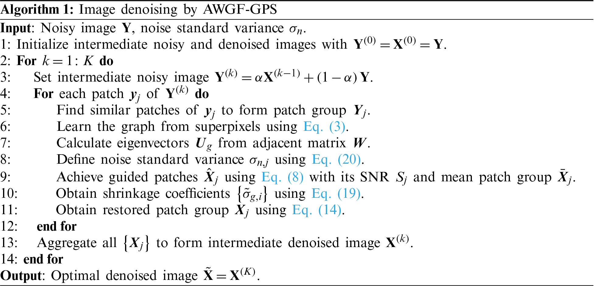
We present the iterative AWGF-GPS denoising framework in Algorithm 1. Given an intermediate noisy image, Y(k), in the k-th iteration, we deal with its j-th noisy patch group, Yj, in four steps.

First, we obtain the Laplacian matrix, L, from the learned superpixel-based graph, W, in Eq. (3) and obtain its graph Fourier bases, Ug. Second, the j-th guided patch group, X^j, is estimated using Eq. (8), where the corresponding SNR, Sj, and the mean patch group, X̄j, are defined by Eqs. (9) and (10), respectively. Here, the noise standard variance, σn,j, of Yj is given by

σn,j=max(σn2-var(Yj-Yj ′),0),(20)

where Yj′ is the patch group of noisy image Y sharing the same patch index of Yj. Third, the AWGF-GPS model is applied to the patch group, Yj, to achieve its shrinkage coefficients {σ̃g,i} using Eq. (19) and the intermediate denoised patches, Xj, using Eq. (14). Finally, we assemble all denoised patches {Xj} into the k-th iterative denoised image, X(k). The optimal denoised image, X̃, is obtained after the K-th iteration.

4  Experimental Results

We compare the AWGF-GPS method with several state-of-the-art model-based denoising methods, including BM3D [12], TWSC [17], ARLLR [18], and AWGF [19]. A deep-learning image denoising method, named the fast and flexible denoising convolutional neural network (FFDNET) [5], is adopted to show the gap between the model-and deep-learning-based denoising methods. Moreover, because our method is derived from AWGF, the denoising parameters are also inherited from those in AWGF. However, for the weighted coefficients in Eq. (13), parameters τ and γ are set as τ=N′σn,j2 and γ=0.1τ-1, respectively. A few clean images are shown in Fig. 2 as test materials. The noisy images are generated by adding Gaussian noise.

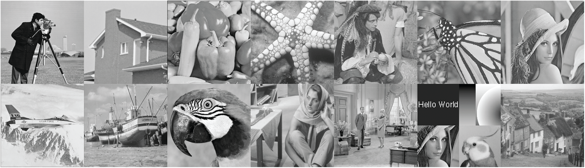
Figure 2: Clean images. From left to right, the images on the top line are named C. Man, House, Peppers, Starfish, Man, Monarch, and Lena, and those on the bottom line are named Airplane, Boats, Parrot, Barbara, Couple, Montage, and Hills

A denoised image comparison of the noise standard deviation of σn=40 is shown in Fig. 3. As a benchmark, BM3D achieves an acceptable denoising performance through collaborative spatial-wavelet filtering. TWSC is better than BM3D with its efficiently learned features of noisy images via sparse representation. ARLLR outperforms the other methods. This indicates that the eigenvalue shrinkage approach is powerful for managing noise. The noise is sufficiently removed in the high “rank-bands” corresponding to the small eigenvalues of the patch group. AWGF emphasizes graph filtering but has less consideration for the image attributes. This leads to a denoising performance that is barely comparable with that of ARLLR. Our method is proven to be the best. The denoised images derived from AWG-GPS are smoothed with a few artificial textures by employing the intra-patch smoothing attribute among the superpixels and the supervision from guided patches. However, FFDNET achieves an outstanding performance in restoring images more naturally. Unlike model-based methods, it benefits from learning the prior from the external images.

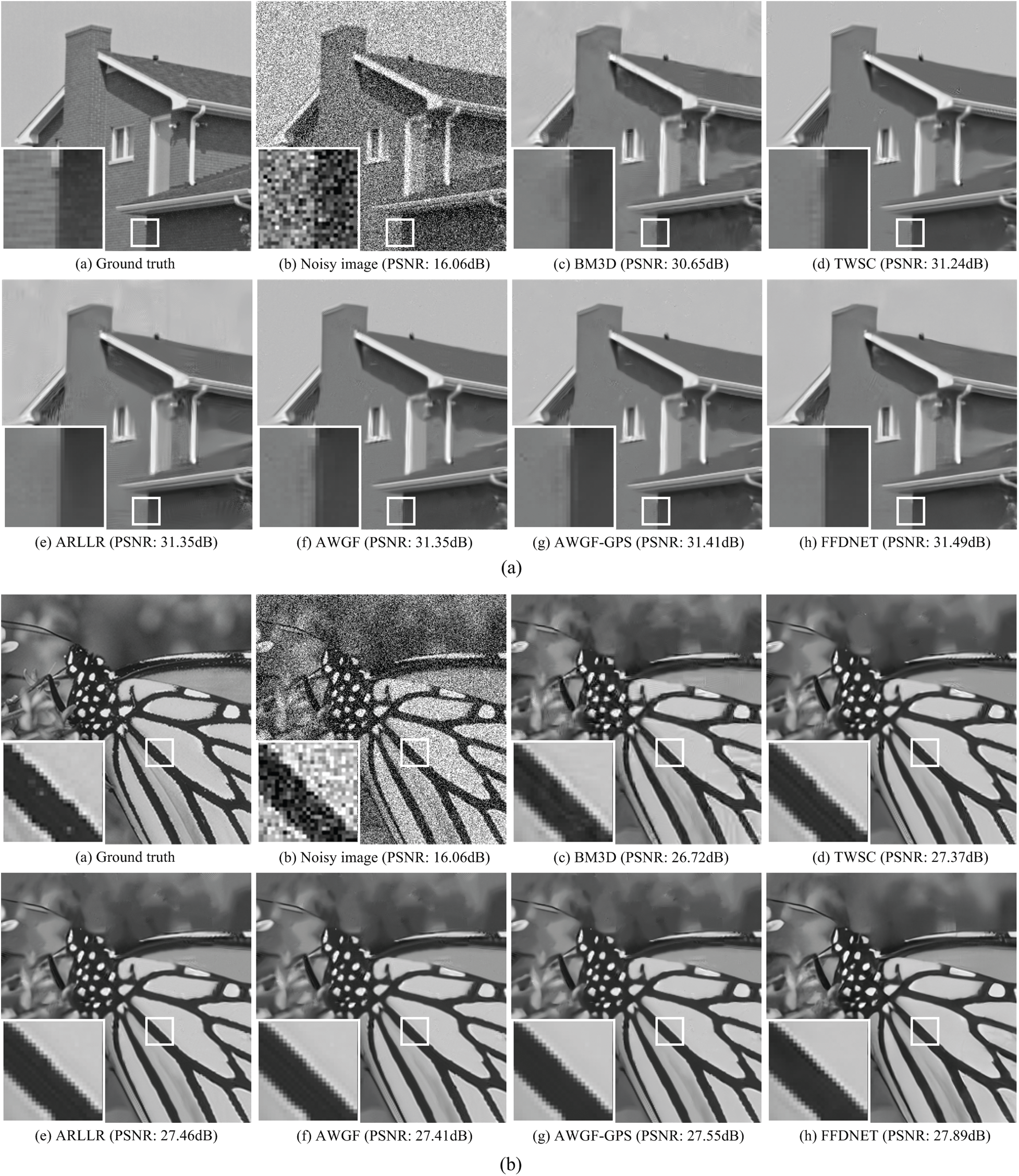
Figure 3: Denoised image comparison of the noise deviation of σn=40. (a) House (b) Monarch

The denoised image comparison of the noise standard deviation of σn=70 is shown in Fig. 4. BM3D obtains good results. TWSC and ARLLR are better than BM3D due to their self-learned features from noisy images. We observe that ARLLR suffers from stronger artificial textures (House). ARLLR is an eigenvalue shrinkage method that uses the statistical information of patch groups via singular value decomposition (SVD). However, it seldom focuses on the pixel smoothing attribute in local areas. AWGF outperforms the aforementioned methods. This proves that graph filtering on the learned graph is useful to alleviate the artificial textures, since the restored patches are required to smoothly evolve on the graph. The proposed AWGF-GPS further smoothens the denoised images, which is owing to the superpixel-based graph, where the similarities between the patches and intra-patch pixels are fully exploited. The shrinkage approach is also efficiently conducted using guided patches. Note that the denoising performance of FFDNET is unsatisfactory. For example, the eaves area of the house is not sufficiently restored. This phenomenon is caused by feature mismatch. In this case, the external prior from the image databases cannot precisely guide the patch reconstruction for denoised images because the features of clean images are significantly contaminated by noise and are difficult to recognize.

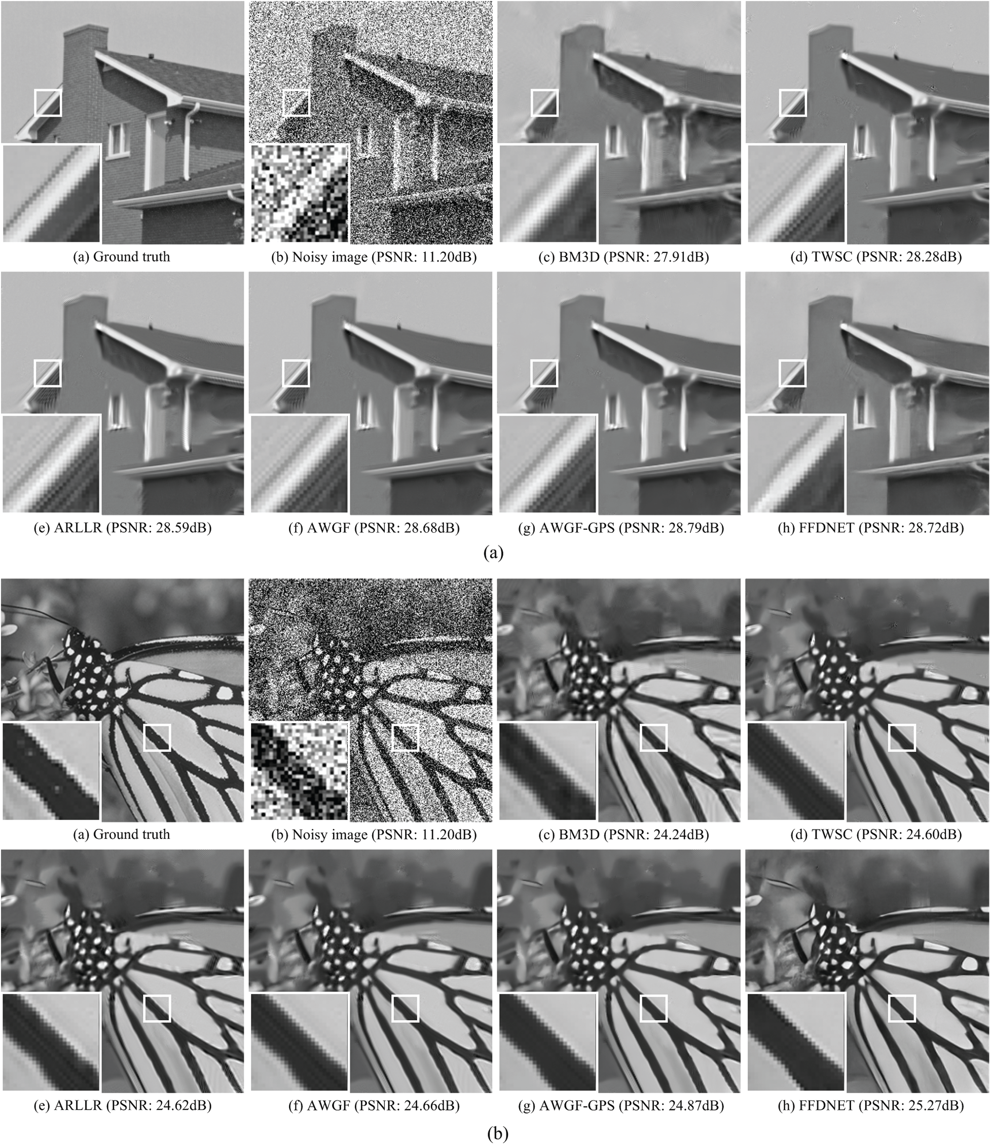
Figure 4: Denoised image comparison of the noise deviation of σn=70. (a) House (b) Monarch

Table 1: PSNR (dB) results of different denoising methods

The statistical results of the PSNR and SSIM are listed in Tabs. 1 and 2. We use BM3D as a baseline, for it achieves an acceptable performance for all the images and noise levels. TWSC outperforms BM3D because it is a learned domain method. In the sparse representation model, dictionary learning aims to catch patch features as atoms, whereas sparse coding focuses on patch restoration. However, as the noise level increases, the performance of the TWSC degenerates significantly. In this case, the atoms are distorted by direct feature learning from the noisy image. ARLLR is better than the former methods. The shrinkage approach on the patch group is effective in dealing with noise because the relationship among patches is exploited. Our AWGF-GPS method performs the best among these model-based denoising methods. As previously indicated, its coefficient shrinkage strategy is presented on the superpixel graph, where both attributes, within and among the patches, are considered. The guided patch regularizer further enhances the denoising performance. We also note that our method may suffer from an over-smoothing problem. It is inappropriate to deal with images (e.g., Barbara) that contain strong textures. The AWGF-GPS model attempts to design a lowpass graph filter. Because the components of the texture are centralized in high graph-frequency bands, the AWGF-GPS filter is unsatisfactory. FFDNET is best in terms of the noise standard deviation of σn≤70 but the worst for σn=100. The use of an external prior is effective in improving denoising performance. However, once the feature mismatch phenomenon occurs, the denoised result significantly deteriorates and becomes inferior to the results of the model-based methods. Compared with FFDNET, our method has the advantage in coping with large noise.

Table 2: SSIM results of different denoising methods

5  Conclusion

We have proposed a guided intra-patch smoothing graph filtering method for single-image denoising. Unlike the traditional AWGF, which only focuses on coefficient shrinkage, the proposed AWGF-GPS method considers more image attributes for denoising. The similarities between patches and intra-patch pixels are exploited by introducing the superpixel operation. Moreover, the guided patches from the MAP estimator provide a reliable optimal direction for the AWGF-GPS model. This provides an additional way to supervise patch restoration during graph filtering. Experiments have demonstrated that the AWGF-GPS method outperforms several state-of-the-art model-based denoising methods and is comparable with certain deep-learning methods.

Funding Statement: This work is supported by Natural Science Foundation of Jiangsu Province, China [BK20170306] and National Key R&D Program, China [2017YFC0306100]. The initials of authors who received these grants are YZ and JL, respectively. It is also supported by Fundamental Research Funds for Central Universities, China [B200202217] and Changzhou Science and Technology Program, China [CJ20200065]. The initials of author who received these grants are YT.

Conflicts of Interest: The authors declare that they have no conflicts of interest to report regarding the present study.

References

 1.  X. Yang, Y. Xu, Y. Quan and H. Ji, “Image denoising via sequential ensemble learning,” IEEE Transactions on Image Processing, vol. 29, pp. 5038–5049, 2020. [Google Scholar]

 2.  K. Jin and S. Wang, “Image denoising based on the asymmetric Gaussian mixture model,” Journal of Internet of Things, vol. 2, no. 1, pp. 1–11, 2020. [Google Scholar]

 3.  F. Zhang, G. Yang and J. Xue, “Hyperspectral image denoising based on low-rank coefficients and orthonormal dictionary,” Signal Processing, vol. 177, no. 1, pp. 107738, 2020. [Google Scholar]

 4.  C. Tian, L. Fei, W. Zheng, Y. Xu, W. Zuo et al., “Deep learning on image denoising: An overview,” Neural Networks, vol. 131, no. 11, pp. 251–275, 2020. [Google Scholar]

 5.  K. Zhang, W. Zuo and L. Zhang, “FFDNet: Toward a fast and flexible solution for CNN-based image denoising,” IEEE Transactions on Image Processing, vol. 27, no. 9, pp. 4608–4622, 2018. [Google Scholar]

 6.  C. Tian, Y. Xu, Z. Li, W. Zuo, L. Fei et al., “Attention-guided CNN for image denoising,” Neural Networks, vol. 124, no. 1–2, pp. 117–129, 2020. [Google Scholar]

 7.  G. Wu, S. Luo and Z. Yang, “Optimal weighted bilateral filter with dual-range kernel for Gaussian noise removal,” IET Image Processing, vol. 14, no. 9, pp. 1840–1850, 2020. [Google Scholar]

 8.  R. Verma and R. Pandey, “Adaptive selection of search region for NLM based image denoising,” Optik, vol. 147, no. 1, pp. 151–162, 2017. [Google Scholar]

 9.  X. Liu and Y. Chen, “NLTV-Gabor-based models for image decomposition and denoising,” Signal Image and Video Processing, vol. 14, no. 2, pp. 305–313, 2020. [Google Scholar]

10. D. Wang, Y. Xiao and Y. Gao, “Image denoising method based on NSCT bivariate model and variational bayes threshold estimation,” Multimedia Tools and Applications, vol. 78, no. 7, pp. 8927–8941, 2019. [Google Scholar]

11. B. Khawla, R. Said and H. Abdeliah, “A wavelet denoising approach based on unsupervised learning model,” EURASIP Journal on Advances in Signal Processing, vol. 2020, no. 36, pp. 1–26, 2020. [Google Scholar]

12. K. Dabov, A. Foi, V. Katkovnik and K. Egiazarian, “Image denoising by sparse 3-D transform-domain collaborative filtering,” IEEE Transactions on Image Processing, vol. 16, no. 8, pp. 2080–2090, 2007. [Google Scholar]

13. A. A. Yahya, J. Tan, B. Su, M. Hu, Y. Wang et al., “BM3D image denoising algorithm based on an adaptive filtering,” Multimedia Tools and Applications, vol. 79, no. 4, pp. 20391–20427, 2020. [Google Scholar]

14. W. Dong, L. Zhang, G. Shi and X. Li, “Nonlocally centralized sparse representation for image restoration,” IEEE Transactions on Image Processing, vol. 22, no. 4, pp. 1620–1630, 2013. [Google Scholar]

15. H. G. Du, “Image denoising algorithm based on nonlocal regularization sparse representation,” IEEE Sensors Journal, vol. 20, no. 20, pp. 11943–11950, 2020. [Google Scholar]

16. Y. Li, G. Gui and X. Cheng, “From group sparse coding to rank minimization: A novel denoising model for low-level image restoration,” Signal Processing, vol. 176, pp. 107655, 2020. [Google Scholar]

17. J. Xu, L. Zhang and D. Zhang, “A trilateral weighted sparse coding scheme for real-world image denoising,” in Proc. European Conf. on Computer Vision, Munich, Germany, pp. 21–38, 2018. [Google Scholar]

18. X. Jia, X. Feng and W. Wang, “Adaptive regularizer learning for low rank approximation with application to image denoising,” in Proc. IEEE Int. Conf. on Image Processing, Seoul, South Korea, pp. 3096–3100, 2016. [Google Scholar]

19. Y. Chen, Y. Tang, L. Zhou, Y. Zhou, J. Zhu et al., “Image denoising with adaptive weighted graph filtering,” Computers, Materials & Continua, vol. 64, no. 2, pp. 1219–1232, 2020. [Google Scholar]

20. A. Ortega, P. Frossard, J. Kovačević, J. M. F. Moura and P. Vandergheynst, “Graph signal processing: Overview, challenges, and applications,” Proceedings of the IEEE, vol. 106, no. 5, pp. 808–828, 2018. [Google Scholar]

21. Y. Fang, H. Zhang and Y. Ren, “Graph regularised sparse NMF factorisation for imagery de-noising,” IET Computer Vision, vol. 12, no. 4, pp. 466–475, 2018. [Google Scholar]

22. X. Zeng, W. Bian, W. Liu, J. Shen and D. Tao, “Dictionary pair learning on Grassmann manifolds for image denoising,” IEEE Transactions on Image Processing, vol. 24, no. 11, pp. 4556–4569, 2015. [Google Scholar]

23. W. Waheed and D. B. H. Tay, “Graph polynomial filter for signal denoising,” IET Signal Processing, vol. 12, no. 3, pp. 301–309, 2018. [Google Scholar]

24. A. C. Yağan and M. T. Özgen, “Spectral graph based vertex-frequency Wiener filtering for image and graph signal denoising,” IEEE Transactions on Signal and Information Processing over Networks, vol. 6, pp. 226–240, 2020. [Google Scholar]

25. Y. Tang, Y. Chen, N. Xu, A. Jiang and Y. Gao, “Image denoising via sparse approximation using eigenvectors of graph Laplacian,” in Proc. Visual Communications and Image Processing, Singapore, pp. 1–4, 2015. [Google Scholar]

26. H. Talebi and P. Milanfar, “Global image denoising,” IEEE Transactions on Image Processing, vol. 23, no. 2, pp. 755–768, 2014. [Google Scholar]

27. F. G. Meyer and X. Shen, “Perturbation of the eigenvectors of the graph Laplacian: Application to image denoising,” Applied and Computational Harmonic Analysis, vol. 36, no. 2, pp. 326–334, 2014. [Google Scholar]

28. Z. Yang, Z. Yang and D. Han, “Alternating direction method of multipliers for sparse and low-rank decomposition based on nonconvex nonsmooth weighted nuclear norm,” IEEE Access, vol. 6, no. 1, pp. 56945–56953, 2018. [Google Scholar]

29. Z. Yang, L. Fan, Y. Yang, Z. Yang and G. Gui, “Generalized singular value thresholding operator based nonconvex low-rank and sparse decomposition for moving object detection,” Journal of the Franklin Institute-Engineering and Applied Mathematics, vol. 356, no. 16, pp. 10138–10154, 2019. [Google Scholar]

30. V. Kalofolias, “How to learn a graph from smooth signals,” Artificial Intelligence and Statistics, vol. 51, pp. 920–929, 2016. [Google Scholar]

31. N. Perraudin, J. Paratte, D. Shuman, L. Martin, V. Kalofolias et al., “GSPBOX: A toolbox for signal processing on graphs,” Eprint Arxiv, vol. 61, no. 7, pp. 1644–1656, 2016. [Google Scholar]

32. M. E. Helou and S. Süsstrunk, “Blind universal bayesian image denoising with gaussian noise level learning,” IEEE Transactions on Image Processing, vol. 29, pp. 4885–4897, 2020. [Google Scholar]

This work is licensed under a Creative Commons Attribution 4.0 International License, which permits unrestricted use, distribution, and reproduction in any medium, provided the original work is properly cited.