[BACK]
Computers, Materials & Continua
DOI:10.32604/cmc.2021.017439 |  |
| Article | |
A Fractional Drift Diffusion Model for Organic Semiconductor Devices
Yi Yang*, Robert A. Nawrocki, Richard M. Voyles and Haiyan H. Zhang
School of Engineering Technology, Purdue University, West Lafayette, 47906, USA
*Corresponding Author: Yi Yang. Email: yang1087@purdue.edu
Received: 30 January 2021; Accepted: 8 March 2021
Abstract: Because charge carriers of many organic semiconductors (OSCs) exhibit fractional drift diffusion (Fr-DD) transport properties, the need to develop a Fr-DD model solver becomes more apparent. However, the current research on solving the governing equations of the Fr-DD model is practically nonexistent. In this paper, an iterative solver with high precision is developed to solve both the transient and steady-state Fr-DD model for organic semiconductor devices. The Fr-DD model is composed of two fractional-order carriers (i.e., electrons and holes) continuity equations coupled with Poisson’s equation. By treating the current density as constants within each pair of consecutive grid nodes, a linear Caputo’s fractional-order ordinary differential equation (FrODE) can be produced, and its analytic solution gives an approximation to the carrier concentration. The convergence of the solver is guaranteed by implementing a successive over-relaxation (SOR) mechanism on each loop of Gummel’s iteration. Based on our derivations, it can be shown that the Scharfetter–Gummel discretization method is essentially a special case of our scheme. In addition, the consistency and convergence of the two core algorithms are proved, with three numerical examples designed to demonstrate the accuracy and computational performance of this solver. Finally, we validate the Fr-DD model for a steady-state organic field effect transistor (OFET) by fitting the simulated transconductance and output curves to the experimental data.
Keywords: Fractional drift diffusion model; Gummel’s iteration; Caputo’s fractional-order ordinary differential equation; organic field effect transistor
1 Introduction
The mathematical modeling of the electrons and holes transports in an inorganic semiconductor (ISC) is established by a system of coupled partial differential equations (PDEs), which are formulated by Gauss’ law applied to the electrical potential φ, and the continuity of the electron and hole current densities, Jn and Jp, respectively [1,2]. Besides modeling of ISCs, this system of coupled PDEs, namely, the drift diffusion (DD) model, has also found extensive applications in modeling other diffusion-reaction processes, such as ion exchanges in the electrochemical solvents [3,4], and the transports of positive/negative particles within cell membranes [5,6]. Depending on different application scenarios, the DD model can be represented in various forms. In the Van Roosbroeck representation of the DD model, the current density equation can be augmented by Einstein’s relation, which gives a fixed proportional relationship between the diffusion coefficients Dp, Dn and the drift mobilities μp, μn [7]. In this paper, the Van Roosbroeck representation of the DD model can be expressed in a closed-form as Eqs. (1)–(3),
−Δ(εφ)=q(p−n+ND+−NA−)(1)
∂n∂t=1q∇⋅Jn+Gn(2)
∂p∂t=−1q∇⋅Jp+Gp(3)
where current densities are given by Jn=−qμnn∇φ+qDn∇n and Jp=−qμpp∇φ−qDp∇p, Einstein’s relations are Dnμn=Dpμp=VT=kTq, VT is the thermal voltage, k is Boltzmann constant, T is the thermal temperature, q is the charge of an electron, ε is semiconductor’s absolute dielectric permittivity, ND+ and NA− are ionized donor and acceptor concentrations. Gn and Gp are the net electron and hole generation rates, respectively. Previous research data collected from Silicon/Germanium test experiments have revealed the effectiveness of the DD model for modeling the charge carrier transports in ISCs [8]. In the past several decades, plentiful numerical algorithms have been developed for solving Eqs. (1)–(3), including the finite element method [9], finite difference fractional step method [10], mixed finite volume and modified upwind fractional difference method [11], and monotone iterative method based on the adaptive finite element discretization [12,13], etc. All of those numerical methods have one thing in common: an efficient iterative method, e.g., Newton’s iteration, Gauss–Seidel iteration, or Gummel’s iteration was utilized to decouple Eqs. (1)–(3). Among these iteration methods, Gummel’s approach is generally more effective than other methods due to its flexibility in finding its initial guess and customizing the update formulas to improve the convergence speed and computational performance. Moreover, the effectiveness, stability and convergence of Gummel’s decoupling method and iteration for its application to DD simulations were also thoroughly and rigorously proved by mathematicians [14–17]. Recent research revealed that the conventional (integer-order) DD model may not be able to characterize the charge carrier transports in organic semiconductors (OSCs), evident from the long-tail behavior of the photocurrent curve observed in OSCs [18]. Based on the DD model, Reference [19] showed that the mean squared displacement (MSD) of the carrier trajectory should be proportional to its diffusion time, i.e., E(x2(t))∝t. However, the long-tail behavior of the photocurrent curve observed in OSCs implies that the MSD in this scenario is given by E(x2(t))∝tα, for α termed as the dispersive parameter of the OSC, 0<α<1, depending on the temperature and band structure disorders [20–23]. This long-tail photocurrent phenomenon was first observed by using time-of-flight measurements [24], and the mechanism that underpins the dispersive carrier transports can be precisely explained by the “multiple trapping model” [23,25], the “single trapping model” [26] and the “hopping model” [27–29], respectively. Based on the “multiple trapping model,” the charge carriers in OSCs can be classified as free (delocalized) charge carriers pf,nf and trap (localized) charge carriers pt, nt. The free charge carrier is the carrier that can hop freely between two trap centers and the trap charge carrier is the carrier that is permanently captured by a localized trap center. References [18,30] proved that the free hole density and the trap hole density in the p-type OSCs have a relationship as given in Eq. (4),
∂pt(x,t)∂t=1τ0cα0RLDtα(pf(x,t))=1τ0cα1Γ(1−α)∂∂t∫0tpf(x,s)(t−s)αds(4)
where 0RLDtα is Riemann–Liouville (RL) fractional derivative of order 0<α<1, τ0 is the mean time of delocalization (mean free time for a free charge carrier moving between two entrapments), c is the charge carrier capture coefficient defined as c=ω0[sin(πα)/πα]α, ω0 is the capture rate of the trap charge carriers, and α=kT/E0 is the dispersive parameter which depends on the temperature T and the expected value of the exponential density of trap states E0. The 1D continuity equation for free charge carriers in p-type OSCs was also derived by References [18,30] as given in Eq. (5),
∂pf(x,t)∂t+1τ0cα0RLDtα(pf(x,t))+∂∂x[μpE(x,t)pf(x,t)]−Dp∂2pf(x,t)∂x2=p(x,0)δ(t)(5)
where E(x,t)=-∂φ(x,t)∂x is the intensity of the electric field in the 1D domain, and p(x,0)δ(t) is the initial charge carriers agitated by impacting of photon beams. Consider that p = pf + pt and pt≫pf in OSCs. Substituting Eq. (4) into Eq. (5) can derive the continuity equation for total charge carrier density, as given in Eq. (6),
0RLDtα(p(x,t))+∂∂x[Fα(x,t)p(x,t)]−Dα∂2p(x,t)∂x2=p(x,0)t−αΓ(1−α)(6)
where Fα(x,t)=τ0cαμpE(x,t) is the anomalous advection coefficient and Dα=τ0cαDp is the anomalous diffusion coefficient. The hole mobility μp and hole diffusion coefficient Dp satisfies the Einstein relation. Eq. (6) coupled with the 1D Poisson equation forms the 1D fractional drift diffusion (Fr-DD) model.1 A discretization scheme, which discretizes the time-fractional derivative with backward finite difference method and the integer-order spatial derivatives with finite center difference method, was proposed to solve the 1D Fr-DD model [20–31]. Reference [20] showed that the photocurrent curves obtained from the 1D Fr-DD model are in good agreement with the recorded transient photocurrents from regio-random OSCs poly(3-hexylthiophene) (RRa-P3HT) and regio-regular poly(3-hexylthiophene) (RR-P3HT). In addition, Reference [32] introduced the fractional reduced differential transform method to solve the 1D Fr-DD model and also suggested the existence of a more general Fr-DD model with both time derivative and spatial derivatives fractionalized. As the Fr-DD model emerges as a useful tool for understanding the dispersive transport behavior of the charge carriers in OSCs, investigating how to solve it is instrumental for predicting the steady-state and transient electrical responses of OSC devices. Up to now, far too little attention has been paid to the development of a general Fr-DD model solver. Although a certain number of researches have been carried out on developing the solvers for the conventional DD model, the resulting solvers often have low accuracy and high computational complexity. The goal of this research is to develop a solver with high precision and computational performance for the Fr-DD model. The Fr-DD model is described by a group of coupled fractional-order PDEs as presented in Eqs. (7)–(9),
−Δ(εφ)=q(p−n)(7)
0CDtα(n(x,y,z,t))=1q∇⋅I+Gn(8)
0CDtα(p(x,y,z,t))=−1q∇⋅J+Gp(9)
where 0CDtα is the Caputo’s time-fractional derivative of order 0<α≤1, the fractional-order electron current density I and hole current density J are given by I=-qμnn∇φ+qDnC∇rβn and J=-qμpp∇φ-qDpC∇rβp, and C∇rβ=(0CDxβ0CDyβ0CDzβ) is the Caputo’s fractional gradient operator of order 0<β≤1 in 3D. Since the OSCs are typically treated as intrinsic materials without dopants, the ionized donors ND+ and acceptors NA- can be omitted in Poisson’s equation [33]. If the fractional-order gradient operator is defined with Riemann–Liouville’s (RL) fractional derivatives, the divergence of current density function ∇⋅J in Eq. (9) can be expanded as ∇⋅J=-qμp(pΔφ+∇p⋅∇φ)-qDpRL∇rβ+1p, similarly for ∇⋅I in Eq. (8) [34,35]. As that defining the fractional derivatives using RL’s definition may not be convenient for us to specify and assign physical meanings to the initial values and boundary conditions, we adopt Caputo’s (C) fractional derivatives to replace RL’s in Eqs. (7)–(9). Since composing Caputo’s fractional derivative with an integer-order gradient operator from its left side may not result in the same expansion as defined by RL’s derivative (See Lemma 2.2), it requires us to show that the truncation error from the discretized divergence term ∇⋅J will vanish as spatial step size reduces to zero to guarantee the consistency of the discretized divergence terms under two different definitions of fractional derivatives (RL’s and Caputo’s). In this paper, we propose Theorem 4.1 to illustrate the consistency of the discretized divergence term ∇⋅J under RL’s and Caputo’s fractional definitions.
Here, we set up a general-form Fr-DD model to simulate the anomalous transport behavior of charge carriers in OSCs. Equipped with proper initial values and boundary conditions, the Fr-DD model can handle the transient or steady-state dynamics of any-type OSC device. In addition, we develop an iterative solver for the Fr-DD model based on two novel algorithms and propose Theorem 4.2 to show the convergence of the model solver. It can be shown that the discretized DD model equation via our discretization scheme coincides with the discrete-form Fr-DD equations derived from the Scharfetter–Gummel (SG) discretization method [9], which implies that our Fr-DD model solver has wider applicability than the DD model solver based on SG method. Finally, we design three numerical examples to demonstrate the high accuracy and computational performance of the Fr-DD model solver, and experimentally validate the Fr-DD model for a steady-state OFET.
The remainder of the paper is organized as follows. Section 2 presents preliminaries in fractional calculus. Section 3 develops the solver in detail. Section 4 discusses the consistency and convergence analysis of the algorithms. Three numerical examples are provided in Section 5 to support our theoretical analysis and demonstrate the computational performance of our method. In Section 6, we adjust the parameters in the Fr-DD model to fit the experimental characteristic curves measured from a DNTT-based OFET [36]. In Section 7, we show the conclusions of this work.
2 Preliminaries
2.1 Definition of Fractional Operators
The Riemann–Liouville (RL) fractional derivative with order γ>0 is defined in Eq. (10) [34],
0RLDtγ(f(t))=1Γ(n−γ)dndtn∫0tf(τ)(t−τ)γ+1−ndτ,n−1<γ<n(10)
where Γ(n-γ) denotes the gamma function. Similarly, Caputo’s fractional derivative with order γ>0 is defined as Eq. (11) [34].
0CDtγ(f(t))=1Γ(n−γ)∫0tf(n)(τ)(t−τ)γ+1−ndτ,n−1<γ<n(11)
Both RL and Caputo’s fractional derivatives can be considered as interpolation to integer-order derivatives, which means 0RLDtn(f(t))=0CDtn(f(t))=f(n)(t). The relationship between RL can Caputo’s fractional derivatives can be expressed as the following lemma.
Lemma 2.1 Assumef∈Cn-1([a,t])andn-1<γ≤n, then the following equality holds
aCDtγ(f(t))=aRLDtγ(f(t))−∑k=0n−1f(k)(a)Γ(k−γ+1)(t−a)k−γ(12)
Proof. See [35].
By directly employing the definitions, the composition rules for fractional derivatives can be given as the following lemma.
Lemma 2.2 Assumef∈Cn+m-1([a,t]), n-1<γ≤n, and m > 0 is an integer, then the following relations hold
dmdtm[aRLDtγ(f(t))]=aRLDtγ+m(f(t))(13)
aCDtγ(dmdtmf(t))=aCDtγ+m(f(t))(14)
aRLDtγ(dmdtmf(t))=aRLDtγ+m(f(t))−∑k=0m−1f(k)(a)Γ(1+k−γ−m)(t−a)k−γ−m(15)
dmdtm[aCDtγ(f(t))]=aCDtγ+m(f(t))+∑k=nn+m−1f(k)(a)Γ(1+k−γ−m)(t−a)k−γ−m(16)
Proof. Eqs. (13) and (14) can be inferred from RL and Caputo’s definitions, and the proof for Eq. (15) is given in [35]. From Lemma 2.1, we haveL{aRLDtγ(f(t))}=sγF(s)−∑k=0n−1sk⋅aRLDtγ−k−1f(a) which completes the proof for Eq. (16).
It can be observed that both RL’s and Caputo’s fractional derivatives can be composed with an integer-order derivative from two sides, but the composition is not commutative. Next, let us give the Laplace transformation on RL and Caputo’s fractional derivatives as the following lemma.
Lemma 2.3 Assumef∈Cn-1([a,t])andn-1<γ≤n, then the Laplace transform of Riemann–Liouville and Caputo’s fractional derivatives are given by
L{ aRLDtγ(f(t)) }=sγF(s)−∑k=0n−1sk⋅aRLDtγ−k−1f(a)(17)
L{aCDtγ(f(t))}=sγF(s)−∑k=0n−1sγ−k−1⋅f(k)(a)(18)
Proof. See [35].
One important formula relating the Laplace transform and two-parameter Mittag–Leffler function is given in Eq. (19), and its proof can be found in [37].
L{tβ−1Eα,β(±atα)}=sα−βsα∓a,R(s)>0,R(α)>0,R(β)>0(19)
Subsequently, we will present the analytic solution for Caputo’s fractional linear time-invariant (LTI) state equation.
2.2 Analytic Solution of Caputo’s Linear Fractional-Order ODE
If we let 0<γ≤1, the analytic solution of Caputo’s linear fractional-order ODE is given in the following theorem.
Theorem 2.4 Consider the Caputo’s linear fractional-order ODE defined in a discrete 1D space domain with x∈[xi-1,xi]and0<γ≤1, as given in Eq. (20), where u(x) is the state variable and v(x) is the input variable.
xi−1CDxγu(x)=Au(x)+Bv(x)(20)
Then, its solution is given by
u(x)=Φ(x−xi−1)u(xi−1)+∫0x−xi−1Φ(x−xi−1−y)Bv^(y)dy(21)
whereΦ(x)=Eγ(Axγ) is the generalized state transition function, Eγ(t) is the one-parameter Mittag–Leffler function, and the fictitious input function v^(y) is obtained by v^(x)=L-1{V(s)s1-γ}.
Proof. Apply Laplace transform on both sides of Eq. (20), it gives
sγU(s)−sγ−1u(xi−1)=AU(s)+BV(s)(22)
Rearrange both sides of Eq. (22) and take the inverse Laplace transform, we haveu(xi)=Φ(Δx)u(xi−1)+B∫0ΔxΦ(y)(Δx−y)γ−1Γ(γ)dy where Id = 1 or Id is the identity matrix in case u,v are vectorized variables. The last step comes from Eq. (19), i.e., the inverse Laplace transform of the Mittag–Leffler function, by letting α=γ and β=1. We also apply the convolution theorem in the last step derivation, and this completes our proof.
The theorem we presented above establishes the precise relationship between states on two consecutive grid points in a 1D discrete space Ωh={xi=iΔx,i=0,1,2,…,N} with step size Δx=L/N. Letting x = xi, we see that two consecutive states have a relation expressed by
u(xi)=Φ(Δx)u(xi−1)+∫0ΔxΦ(Δx−y)Bv^(y)dy(23)
Let us assume that the input function v(t)=1, the fictitious input function is then evaluated by v^(y)=L-1{s-γ}=yγ-1Γ(γ), and considering the commutative property of the convolution integral, then Eq. (23) in this special case can be reformulated as
u(xi)=Φ(Δx)u(xi−1)+B∫0ΔxΦ(y)(Δx−y)γ−1Γ(γ)dy(24)
We notice that the second term on the RHS of Eq. (24) involves a fractional integral of order γ. The fractional integral (or the left Riemann–Liouville integral) of order γ is defined as Eq. (25). [38]
J0+γf(x)=1Γ(γ)∫0xf(y)(x−y)1−γdy(25)
In the next section, we present discrete approximation formula for the left Riemann–Liouville integral and fractional derivatives.
2.3 Discrete Approximation of Fractional Integrals and Fractional Derivatives
The fractional integral of the generalized state transition function cannot be evaluated through an analytic formula. The following lemma gives the composite Simpson’s rule for approximating a left Riemann–Liouville integral.
Lemma 2.5 Assume0<γ≤1andf∈C4([0,x]) then the following (3+γ)-th order approximation of the left Riemann–Liouville integral can be obtained
J0+γf(x)=(Δx)γ[∑k=0nb2k(γ)f(x2k)+∑k=1nb2k−1(γ)f(x2k−1)]+O(Δx3+γ)(26)
wherexj=jΔx with a positive integer j and step size Δx. Since we let x = x2n, the coefficients bj(γ) satisfies following formula,
b2k−1(γ)=−2(2n−2k+2)2+γ−(2n−2k)2+γΓ(3+γ)+2(2n−2k+2)1+γ+(2n−2k)1+γΓ(2+γ)(27)
b2k(γ)={ (2n)2+γ−(2n−2)2+γΓ(3+γ)−3(2n)1+γ+(2n−2)1+γ2Γ(2+γ)+(2n)γΓ(1+γ), k=0(2n−2k+2)2+γ−(2n−2k−2)2+γΓ(3+γ)−(2n−2k+2)1+γ+6(2n−2k)1+γ+(2n−2k−2)1+γ2Γ(2+γ),360ptk=1,…,n−122+γΓ(3+Γ)−21+γ2Γ(2+γ), k=n (28)
Proof. See [39].
For the transient-state Fr-DD model, the discretization of the time-fractional derivative is necessary, the following lemma gives a first-order approximation for Caputo’s fractional time derivative of order 0<γ≤1.
Lemma 2.6 Assume0<γ≤1andf∈C2([0,T]) then the following first-order approximation of the Caputo’s time-fractional derivative can be obtained
0CDtγ(f(t))=1Γ(2−γ)∑m=0kf(tk+1−m)−f(tk−m)Δtγbm,k+1(γ)+O(Δt)(29)
wheretj=jΔt with a positive integer j and step size Δt. Since we let T = tk+1, the coefficients bm,k+1(γ) is determined by
bm,k+1(γ)=(m+1)1−γ−m1−γ(30)
Proof. The discrete approximation in Eq. (29) can be constructed by applying the piecewise quadrature, the error estimates can be derived as follows,φk|∂ΩD=fφ(∂ΩD),k=0,1,…,N where the mean value theorem is applied for f(t) and f′(t) with ξ1, ξ2∈(tm,tm+1), and the continuous function f(2) on a compact domain [0,T] assumes its maximum value, we let M= maxt∈[0,T]f(2)(t).
3 Derivation of the Computational Scheme
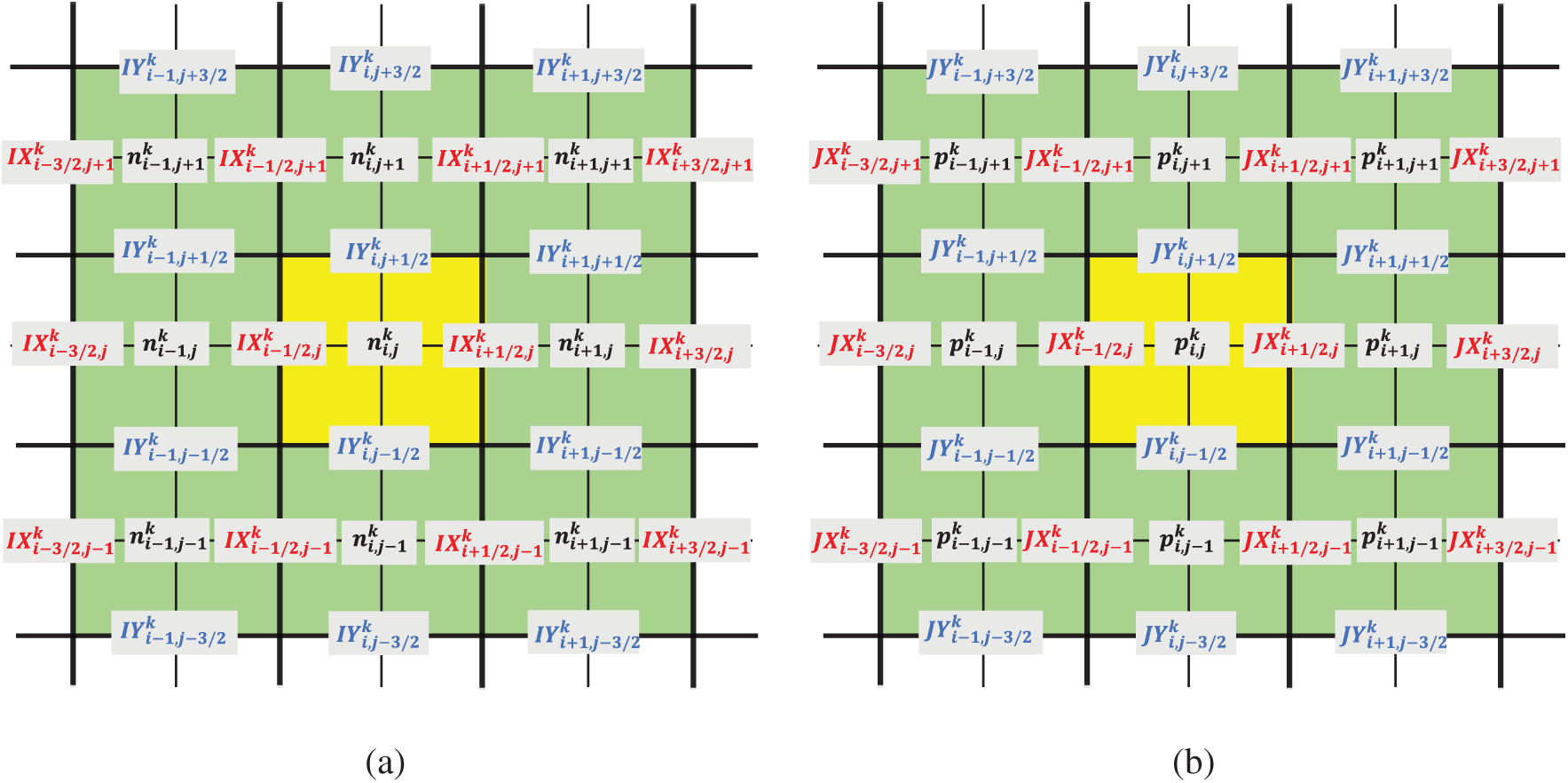
Without loss of the generality, we implement the discretization schemes in the two-dimensional spatial domain, the equations and algorithms derived afterward can be extended to one-dimensional and three-dimensional scenarios. Let the spatial step size in the x direction be Δx=Lx/(Nx+1) and in the y direction be Δy=Ly/(Ny+1). The two-dimensional grids are given by xi=iΔx,i=0,1,…,Nx+1 and yj=jΔy,j=0,1,…,Ny+1. In the temporal domain, we let the temporal step size be Δt=T/N, and the temporal girds are then determined by tn=nΔt,n=0,1,2,…,N. For the sake of a clear demonstration, a set of notations for the charge carrier concentrations and current densities in the 2D discrete domain are presented in Fig. 1. As shown in Fig. 1a, the electron concentration n(tk,xi,yj) and the two components of the electron current density vector (IX(tk,xi+1/2,yj), IY(tk,xi,yj+1/2)) in the discretized electron continuity equation are denoted by ni,jk and (IXi+1/2,jk,IYi,j+1/2k), respectively. Also, Fig. 1b records a similar set of notations employed in the discretized hole continuity equation for the hole concentration p and two components of the hole current density vector (JX,JY). In contrast to the charge carrier concentration, it is required in the scheme that the current density should be specified only in the semi-grids (the midpoints of two horizontally or vertically consecutive normal grids). In the discretized Poisson equation, the electrostatic potentials φi,jk are specified in the normal grids. However, in case the underpinned material is inhomogeneous, the dielectric permittivity is not a constant within the material domain and its spatially distributed values εi+1/2,j+1/2 should be assigned in the semi-grids (the midpoints of two diagonally consecutive normal grids) in our discretization scheme. The notations for the discrete electrostatic potentials and the spatially distributed dielectric permittivity values are not depicted in Fig. 1 due to the space limitation for demonstration. In the following sections, we derive the computational schemes for the transient and steady-state Fr-DD model separately.
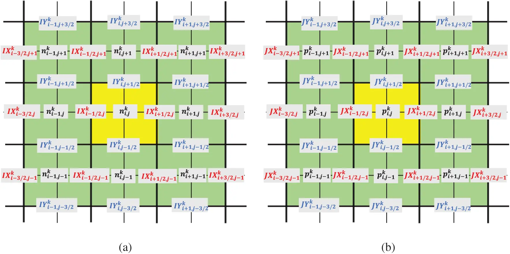
Figure 1: An illustration of notations in the discrete space for (a) discretized electron continuity equation with electron concentration ni,jk, x-direction component of electron current density IXi,jk, and y-direction component of electron current density IYi,jk; (b) discretized hole continuity equation with hole concentration pi,jk, x-direction component of hole current density JXi,jk, and y-direction component of hole current density JYi,jk
3.1 Discretization of Fr-DD Model in Transient State
For Poisson equation, we directly apply the second-order finite central difference on the Laplace operator, then Eq. (7) becomes
ε~i−1,jφi−1,jk−ε~i,j,1φi,jk+ε~i+1,jφi+1,jkΔx2+ε~i,j−1φi,j−1k−ε~i,j,2φi,jk+ε~i,j+1φi,j+1kΔy2=−q(pi,jk−ni,jk)(31)
where the generalized dielectric coefficients are given by ε̃i-1,j=εi-1/2,j-1/2+εi-1/2,j+1/22, ε̃i+1,j=εi+1/2,j-1/2+εi+1/2,j+1/22, ε̃i,j,1=ε̃i-1,j+ε̃i+1,j, ε̃i,j-1=εi+1/2,j-1/2+εi-1/2,j-1/22, ε̃i,j+1=εi+1/2,j+1/2+εi-1/2,j+1/22, and ε̃i,j,2=ε̃i,j-1+ε̃i,j+1. For i=1,2,…,Nx and j=1,2,…,Ny, at each time step tk, k=1,…,N, rearranging Eq. (31) gives a matrix equation Aφφ(k)=bφ(k), where Aφ∈ℝNxNy×NxNy is a pentadiagonal matrix composed of dielectric permittivity constants, φ(k)=[φ1,1k,φ2,1k,⋯,φNx,Nyk]T is the unknown electrostatic potentials inside the boundary and bφ(k)∈ℝNxNy is the vector composed of electric charges and known electrostatic potentials on the boundary. Depending on the types of boundary conditions, the electrostatic potentials on the boundary should be either updated repeatedly at each time step or updated just once at the initial time step. The Dirichlet boundary conditions are given as follows:
φk|∂ΩD=fφ(∂ΩD), k=0,1,…,N(32)
where fφ(∂ΩD) is a predefined function on the Dirichlet boundary ∂ΩD. The Neumann or Robin boundary conditions, as given in Eq. (33), should be updated repeatedly at each time step.
φk|∂ΩN=gφ(φk−1|Ω),k=0,1,…,N(33)
where gφ(φk-1|Ω) is a function defined on the interior discrete points, and the form of gφ is given by discretizing the continuous Neumann or Robin boundary conditions.
For the electron continuity equation, the diffusion coefficient Dp, Dn and carrier mobility μp, μn can be spatially distributed, so they can be parameterized as similar as the dielectric permittivity and form four independent parameter matrices. Nevertheless, in the ensuing derivations, we treat Dp,Dn,μp and μn as constants within the whole domain in order to reduce the indicial complexity.
For Caputo’s space-fractional gradient operator in the electron continuity equation, firstly we will treat the current density flowing through the interval of two consecutive normal grids as a constant, which can result in two Caputo’s linear fractional-order ODEs (assume that the time step is at k + 1):
IXi−1/2,jk+1=−qμnn∂φ∂x+qDn⋅xi−1CDxβn(34)
IYi,j−1/2k+1=−qμnn∂φ∂y+qDn⋅yi−1CDxβn(35)
Referring to Eq. (24) and Theorem 2.4, the solutions to these two fractional-order ODEs can be obtained as follows:
ni,jk+1=Φ2(Δx)ni−1,jk+1+IXi−1/2,jk+1qDnJ0+βΦ2(Δx)(36)
ni,jk+1=Φ1(Δy)ni,j−1k+1+IYi,j−1/2k+1qDnJ0+βΦ1(Δy)(37)
where the generalized state transition functions are defined by
Φ2(t)=Eβ(φi,jk+1−φi−1,jk+1VTtβ−1)(38)
Φ1(t)=Eβ(φi,jk+1−φi,j−1k+1VTtβ−1)(39)
In Eq. (8), the gradient of current density is approximated by ∇⋅I=IXi+1/2,jk+1-IXi-1/2,jk+1Δx+IYi,j+1/2k+1-IYi,j-1/2k+1Δy. By substituting IXi+1/2,jk+1, IXi-1/2,jk+1, IYi,j+1/2k+1 and IYi,j-1/2k+1 into Eq. (8) and approximating the time-fractional derivative using Lemma 2.6, we can get the discrete form of Eq. (8) as follows:
1Γ(2−α)∑m=0kni,jk+1−m−ni,jk−mΔtαbm,k+1(α)=Ci,j−1k+1ni,j−1k+1+Ci−1,jk+1ni−1,jk+1+Ci,jk+1ni,jk+1+Ci+1,jk+1ni+1,jk+1+Ci,j+1k+1ni,j+1k+1+Gn(40)
where bm,k+1(α)=(m+1)1-α-m1-α, and coefficients Ci,j-1k+1, Ci-1,jk+1, Ci,jk+1, Ci+1,jk+1 and Ci,j+1k+1 are given in Eqs. (41)–(45),
Ci,j−1k+1=Φ1(Δy)J0+βΦ1(Δy)DnΔy(41)
Ci−1,jk+1=Φ2(Δx)J0+βΦ2(Δx)DnΔx(42)
Ci,jk+1=[−1J0+βΦ2(Δx)−Φ3(Δx)J0+βΦ3(Δx)]DnΔx+[−1J0+βΦ1(Δy)−Φ4(Δy)J0+βΦ4(Δy)]DnΔy(43)
Ci+1,jk+1=1J0+βΦ3(Δx)DnΔx(44)
Ci,j+1k+1=1J0+βΦ4(Δy)DnΔy(45)
where the generalized state transition functions Φ1(t) and Φ2(t) are given in Eqs. (38) and (39), while Φ3(t) and Φ4(t) are given by
Φ3(t)=Eβ(φi+1,jk+1−φi,jk+1VTtβ−1)(46)
Φ4(t)=Eβ(φi,j+1k+1−φi,jk+1VTtβ−1)(47)
For the left Riemann–Liouville integrals appearing in Eqs. (41)–(45), the three-point Simpson’s rule inferred by Lemma 2.5 can be applied to obtain their approximated values to order of 3+β. For instance, J0+βΦ1(Δy) is approximated by
J0+βΦ1(Δy)=(Δy)β2Γ(β)[(1−2Φ1(Δy2)+Φ1(Δy))(4β−8β+1+4β+2)−(−3−4Φ1(Δy2)+Φ1(Δy))(2β−2β+1)−4β](48)
The other Riemann–Liouville integrals J0+βΦ2(Δx), J0+βΦ3(Δx), and J0+βΦ4(Δy) can thus be approximated accordingly. As a result, Eq. (40) can then be arranged in a matrix form An(k+1)n(k+1)=bn(k+1), where An(k+1) is a pentadiagonal matrix, n(k+1) is the unknown interior electron concentrations at the (k+1)-th time step, bn(k+1) is a column vector composed of the known boundary electron concentration at the (k+1)-th time step and the known interior electron concentrations solved from the previous k time steps.
The hole continuity equation in Eq. (9) can also be discretized with a similar procedure, and its discrete form is obtained in Eq. (49),
1Γ(2−α)∑m=0kpi,jk+1−m−pi,jk−mΔtαbm,k+1(α)=Di,j−1k+1pi,j−1k+1+Di−1,jk+1pi−1,jk+1+Di,jk+1pi,jk+1+Di+1,jk+1pi+1,jk+1+Di,j+1k+1pi,j+1k+1+Gp(49)
where coefficients Di,j-1k+1, Di-1,jk+1, Di,jk+1, Di+1,jk+1 and Di,j+1k+1 are given in Eqs. (50)–(54).
Di,j−1k+1=Φ^1(Δy)J0+βΦ^1(Δy)DpΔy(50)
Di−1,jk+1=Φ^2(Δx)J0+βΦ^2(Δx)DpΔx(51)
Di,jk+1=[−1J0+βΦ^2(Δx)−Φ^3(Δx)J0+βΦ^3(Δx)]DpΔx+[−1J0+βΦ^1(Δy)−Φ^4(Δy)J0+βΦ^4(Δy)]DpΔy(52)
Di+1,jk+1=1J0+βΦ^3(Δx)DpΔx(53)
Di,j+1k+1=1J0+βΦ^4(Δy)DpΔy(54)
where we denote the generalized reversed state transition functions by Φ^1(t), Φ^2(t), Φ^3(t) and Φ^4(t), and their definitions are given by Eqs. (55)–(58). Similarly, the left Riemann-Liouville integrals of the generalized state transition functions can also be approximated by three-point Simpson’s rule.
Φ^1(t)=Eβ(−φi,jk+1−φi,j−1k+1VTtβ−1)(55)
Φ^2(t)=Eβ(−φi,jk+1−φi−1,jk+1VTtβ−1)(56)
Φ^3(t)=Eβ(−φi+1,jk+1−φi,jk+1VTtβ−1)(57)
Φ^4(t)=Eβ(−φi,j+1k+1−φi,jk+1VTtβ−1)(58)
As remarkably similar in format to Eqs. (40), (49) can also be transformed into a compact matrix equation Ap(k+1)p(k+1)=bp(k+1). The boundary conditions for these linear matrix equations are then specified as follows:
nk|∂ΩD=fn(∂ΩD),nk|∂ΩN=gn(nk−1|Ω),k=0,1,…,N(59)
pk|∂ΩD=fp(∂ΩD),pk|∂ΩN=gp(pk−1|Ω),k=0,1,…,N(60)
ni,j0=hn(xi,yj),pi,j0=hp(xi,yj),i=0,1,…,Nx+1;j=0,1,…,Ny+1(61)
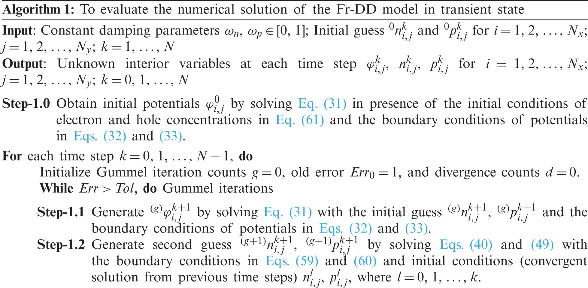
where fn, fp are the predefined functions in Dirichlet boundary conditions, and gn, gp are the functions derived from the Neumann or Robin boundary conditions. Furthermore, the initial value conditions are specified in Eq. (61). Given the discrete form of the transient-state Fr-DD model in Eqs. (31), (40) and (49) and the consistency between the initial value and boundary conditions, we propose Algorithm 1 to solve the unknowns φ,n and p for each time step.

3.2 Discretization of Fr-DD Model in Steady State
Since Caputo’s fractional derivative of any constant is zero, the time-derivative term with Caputo’s fractional derivatives vanishes in steady state. In contrast to the transient-state Fr-DD model, the discretized steady-state Fr-DD model is formed by Eqs. (31), (62) and (63).
Ci,j−1k+1ni,j−1k+1+Ci−1,jk+1ni−1,jk+1+Ci,jk+1ni,jk+1+Ci+1,jk+1ni+1,jk+1+Ci,j+1k+1ni,j+1k+1=−Gn(62)
Di,j−1k+1pi,j−1k+1+Di−1,jk+1pi−1,jk+1+Di,jk+1pi,jk+1+Di+1,jk+1pi+1,jk+1+Di,j+1k+1pi,j+1k+1=−Gp(63)
The boundary conditions for Poisson’s equation and the carrier continuity equations are specified in Eqs. (32), (33), (59) and (60). By rearranging Eqs. (31), (62) and (63), three matrix equations, i.e., Aφφ=bφ, Ann = bn and App = bp, can be formed for algebraic computations. As a result, we propose Algorithm 2 to solve the numerical solution of the steady-state Fr-DD model.
3.3 Special Case when α=1 and β=1
When α=1 and β=1, the Fr-DD model becomes the conventional DD model which is universally employed in the modeling of crystalline semiconductors (e.g., Si, Ge, etc.). In this case, through simple calculations and substitutions, it can be verified that Eqs. (40) and (49) degenerate into Eqs. (64) and (65), respectively.
ni,jk+1−ni,jkΔt=−μnVTΔx2[B(i−1,i),jk+1ni−1,jk+1−(B(i,i−1),jk+1+B(i,i+1),jk+1)ni,jk+1+B(i+1,i),jk+1ni+1,jk+1]−μnVTΔy2[Bi,(j−1,j)k+1ni,j−1k+1−(Bi,(j,j−1)k+1+Bi,(j,j+1)k+1)ni,jk+1+Bi,(j+1,j)k+1ni,j+1k+1]+Gn(64)
pi,jk+1−pi,jkΔt=μpVTΔx2[B(i,i−1),jk+1pi−1,jk+1−(B(i−1,i),jk+1+B(i+1,i),jk+1)pi,jk+1+B(i,i+1),jk+1pi+1,jk+1]+μpVTΔy2[Bi,(j,j−1)k+1pi,j−1k+1−(Bi,(j−1,j)k+1+Bi,(j+1,j)k+1)pi,jk+1+Bi,(j,j+1)k+1pi,j+1k+1]+Gp(65)
where the new coefficients are defined as B(n,m),jk+1=B(φn,jk+1-φm,jk+1VT) and Bi,(n,m)k+1=B(φi,nk+1-φi,mk+1VT), within which B(x)=xexp(x)-1 is the Bernoulli function. Here the discretized system of equations formed by Eqs. (31), (64) and (65) is identical to the discretized system of equations derived from the well-known Scharfetter–Gummel method [9]. Likewise, Algorithm 1 and 2 can be easily modified to solve the numerical solution of the conventional DD model.
4 Consistency and Convergence Analysis
The proposed discretization scheme is consistent if the truncation error terms can be made to vanish as the mesh and time step size is reduced to zero. First of all, the consistency of the finite center difference scheme applied to the Poisson equation can be easily proved [40]. Furthermore, it can be inferred from Lemma 2.5 and Lemma 2.6 that the truncation error of the discretized carrier continuity equations in Eqs. (40) and (49) will vanish as the spatial and time step sizes shrink to zero. Nevertheless, Eq. (16) hints that an additional truncation error can be generated by composing Caputo’s fractional derivative terms in the current density with an integer-order gradient operator on the left side of the equation. To test the influence of this truncation error on the consistency of Eqs. (40) and (49), we propose Theorem 4.1, which gives the shrinking order of this truncation error with the spatial step sizes.
Theorem 4.1 Consider the two-dimensional divergence terms ∇⋅Iand∇⋅J in Eqs. (8) and (9) with I=-qμnn∇φ+qDnC∇rβnandJ=-qμpp∇φ-qDpC∇rβp, then the following equations hold for 0<β<1.
∇⋅I=−qμn(nΔφ+∇n⋅∇φ)+qDnC∇rβ+1n+∇⋅[∂n∂x|0x1−βΓ(2−β)ix+∂n∂y|0y1−βΓ(2−β)iy](66)
∇⋅J=−qμp(pΔφ+∇p⋅∇φ)−qDpC∇rβ+1p−∇⋅[∂p∂x|0x1−βΓ(2−β)ix+∂p∂y|0y1−βΓ(2−β)iy](67)
whereix,iy are unit vector in the x and y direction.
Proof. Observing that both equations are similar in structure and symmetric in x and y directions, it is sufficient to prove Eq. (66) in only the x direction. From Eq. (12), we obtain
0CDxβ(n(x,y))=0RLDxβ(n(x,y))−n(0,y)Γ(1−β)x−β(68)
If we take the first derivative of both sides of Eq. (68), we can obtain
∂[0CDxβ(n(x,y))]∂x=0RLDxβ+1(n(x,y))+βn(0,y)Γ(1−β)x−β−1(69)
According to Eq. (12), 0RLDxβ+1(n(x,y)) can be expanded as
0RLDxβ+1(n(x,y))=0CDxβ+1(n(x,y))+n(0,y)Γ(−β)x−(β+1)+∂n∂x|0Γ(1−β)x−β(70)
Substituting Eq. (70) into Eq. (69) and observing that Γ(1-β)=-βΓ(-β), we can obtain
∂[0CDxβ(n(x,y))]∂x=0CDxβ+1(n(x,y))+∂n∂x|0Γ(1−β)x−β(71)
Then we can see Eq. (66) as a corollary to Eq. (71). This completes the proof.
In the derivation of Eqs. (40) and (49), we treat current I and J as constants and solve Caputo’s linear fractional-order ODE within two consecutive grid points. Therefore, from Theorem 4.1, we can get
∇⋅[I¯−∂n∂x|xiΔx1−βΓ(2−β)ix−∂n∂y|yjΔy1−βΓ(2−β)iy]=[−qμn(nΔφ+∇n⋅∇φ)+qDnC∇rβ+1n]i,j(72)
where I¯=(IXi+1/2,j,IYi,j+1/2) is the augmented electron current density vector. Eq. (72) shows that the discretized current density terms can be composed with an integer-order gradient operator from the left with an inclusive truncation error. By forcing Δx,Δy→0, these truncation error terms will decay with the spatial step size to a fractional order 1-β. This then consolidates our claims on the consistency of the proposed discretization scheme.
For convenience, the convergence analysis is only performed on Algorithm 2, but the conclusions of the analysis also apply to Algorithm 1 due to its structural similarity to Algorithm 2 within each step of time advancement. Let us begin our analysis by setting up a finite dimensional vector space V:={φ∈ℝNxNy:∥φ∥∞<∞} and a product vector space Y:={[n,p]∈ℝNxNy×ℝNxNy:∥n∥∞<∞,∥p∥∞<∞}. The Gummel map is a mapping A:Y→V×Y that relates a pair [n1,p1] to a triplet (φ,n2,p2). Therefore, the Gummel mapping in Algorithm 2 can be represented by a series of linear matrix computations in Eqs. (73)–(75),
Aφ⋅(g)φ=bφ((g)n,(g)p,φ|∂Ω)(73)
An((g)φ)⋅(g+1)n^=bn((g)φ,n|∂Ω)(74)
Ap((g)φ)⋅(g+1)p^=bp((g)φ,p|∂Ω)(75)
where ((g)φ,(g+1)n,(g+1)p)=A[ (g)n,(g)p ]. We need to show that the Gummel mapping is a contraction mapping with contraction constant L < 1, and the fixed point theorem guarantees the convergence of the algorithms.
Theorem 4.2 The Gummel mapping A is a contraction mapping if we consider the successively over relaxation mechanism in the Gummel iteration.
Proof. substitute (g)φ into Eqs. (74) and (75), we have
(g+1)n^=An−1(Aφ−1bφ((g)n,(g)p,φ|∂Ω))bn(Aφ−1bφ((g)n,(g)p,φ|∂Ω),n|∂Ω)(76)
(g+1)p^=Ap−1(Aφ−1bφ((g)n,(g)p,φ|∂Ω))bp(Aφ−1bφ((g)n,(g)p,φ|∂Ω),p|∂Ω)(77)
By damping the intermediate results, we can get
(g+1)n=ωn⋅An−1(Aφ−1bφ((g)n,(g)p,φ|∂Ω))bn(Aφ−1bφ((g)n,(g)p,φ|∂Ω),n|∂Ω)+(1−ωn)⋅(g)n(78)
(g+1)p=ωp⋅Ap−1(Aφ−1bφ((g)n,(g)p,φ|∂Ω))bp(Aφ−1bφ((g)n,(g)p,φ|∂Ω),p|∂Ω)+(1−ωp)⋅(g)p(79)
Taking quotient on both sides and applying triangular inequality yield
‖A‖≤ωn‖An−1(Aφ−1bφ((g)n,(g)p,φ|∂Ω))bn(Aφ−1bφ((g)n,(g)p,φ|∂Ω),n|∂Ω)‖‖(g)n‖+1−ωn(80)
‖A‖≤ωp‖Ap−1(Aφ−1bφ((g)n,(g)p,φ|∂Ω))bp(Aφ−1bφ((g)n,(g)p,φ|∂Ω),p|∂Ω)‖‖(g)p‖+1−ωp(81)
Since the relative sizes of (g+1)n^ and (g+1)p^ to (g)n and (g)p are indeterminable, we need to discuss the following two cases. For ‖ (g+1)n^ ‖≥‖ (g)n ‖ and ‖ (g+1)p^ ‖≥‖ (g)p ‖, Steps 1.4–1.6 in Algorithm 2 imply that ωn→0 and ωp→0 if divergence count d exceeds 1000. Therefore, ∥A∥≤1 and iteration converge in large g. For ‖ (g+1)n^ ‖<‖ (g)n ‖ or ‖ (g+1)p^ ‖<‖ (g)p ‖, it can be inferred from Eqs. (80) and (81) that ∥A∥<1. This completes the proof.
5 Numerical Examples
In this section, we consider three numerical examples to evaluate the accuracy and demonstrate the computational performance of our Fr-DD model solver. All the numerical computations below are based on a MATLAB (R2019b) subroutine and performed on a laptop (MacBook Pro 2019) with Intel Core i9 CPU and 16 GB of RAM.
Example 5.1 Consider the following single-carrier transport problem with fractional derivatives in both time and space for (x,y)∈Ω and t > 0.
−Δφ=∇⋅u_=−n(82)
f(x,y,t)=−2π2t1−αE1,2−α(−2π2t)sin(πx)sin(πy)−k2exp(−4π2t)(cos(2πx)sin2(πy)+sin2(πx)cos(2πy))−exp(−2π2t)[πβ+1sin(πx+(β+1)π2)sin(πy)+πβ+1sin(πy+(β+1)π2)sin(πx)](83)
where Ω=(0,1)×(0,1), 0<α≤1, and 0<β≤1. The exact solution to this problem is prescribed as φ=-12π2 exp(-2π2t)sin(πx)sin(πy) and n= exp(-2π2t)sin(πx)sin(πy), where the nonlinear term on the RHS of Eq. (83) is then given by
f(x,y,t)=−2π2t1−αE1, 2−α(−2π2t)sin(πx)sin(πy)−k2exp(−4π2t)( cos(2πx)sin2(πy) +sin2(πx)cos(2πy) )−exp(−2π2t) [ πβ+1sin( πx +(β+1)π2 )sin(πy)+πβ+1sin(πy+(β+1)π2)sin(πx) ]
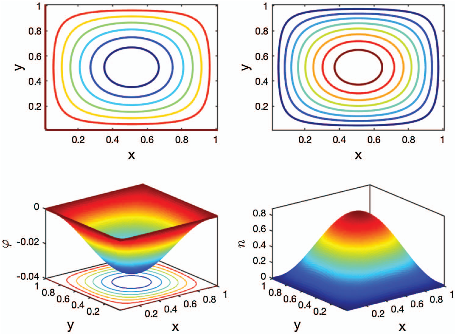
Example 5.1 is a benchmark problem constructed by the method of manufactured solutions [41]. The ground truth is known with its solutions at t = 0.02 s sketched in Fig. 2. The ground truth is compared to the numerical solutions to evaluate the convergence order of our algorithms. The error in this example is calculated by a variant form of the Frobenius norm acting on the error matrix, i.e., e(τ,Δx,k)=1N2∑i=1N∑j=1N|ni,jk-n(iΔx,jΔx,kτ)|2. Here, the spatial step sizes in x and y dimensions are both given by Δx=1/(N+1), where N is the number of internal grid points in one dimension.
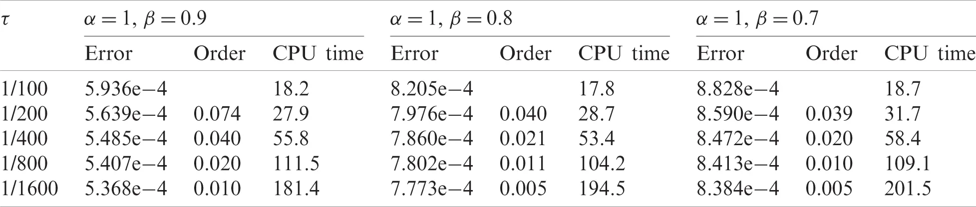
To verify the convergence order in time, we make the spatial step size Δx small enough, such as Δx=0.01 in this case, to ensure that the spatial discretization error is much smaller than the time discretization error. With different temporal step sizes τ, the numerical errors and the CPU times can be obtained and are shown in Tabs. 1 and 2, respectively. In Tab. 1, we compare three different combinations of α and β for fixed β=1, and it is observed that most of the numerical convergence orders in time lie within (1,2). This observation gives an estimate for the convergence order in time and shows its dependence on the time-derivative order α. In Tab. 2, we compare three different combinations of α and β for fixed α=1. With space-derivative order β varying, the convergence orders in time approach zero, implying the negligent effect of β on the convergence order in time. The overall error of our discretization scheme is dominated by the approximation error of the Riemann–Liouville integral (See Eq. (48)), as the approximation error of the Riemann–Liouville integral is only determined by the β value and the spatial step size Δx. Therefore, as the temporal step size τ shrinks the error in Tab. 2 remains relatively unchanged. The overall error can be further decreased by reducing the spatial step size Δx, which is consistent with the trend observed in Tab. 4. However, it should be mentioned that the approximation of the Riemann–Liouville integral will not limit the overall accuracy of the scheme in the case of β=1 (See Tab. 1) since we can analytically calculate the Riemann–Liouville integral when β=1. In addition, it can also be observed in Tabs. 1 and 2 that the speed at which the CPU time increases is less than the speed at which the temporal step size shrinks suggesting that the computational error of the solver can be reduced to any pre-set magnitude at the cost of a relatively small increase in CPU time.
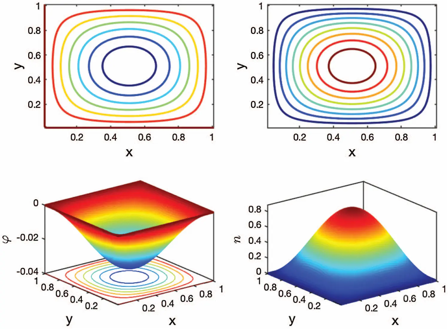
Figure 2: The contour plots (top) and surface plots (bottom) of the electric potentials (left) and the electron concentrations (right) at t = 0.02 s
Table 1: The errors, numerical convergence orders in time and CPU times for different temporal step sizes τ with fixed spatial step size Δx=0.01 and fixed space-derivative order β=1
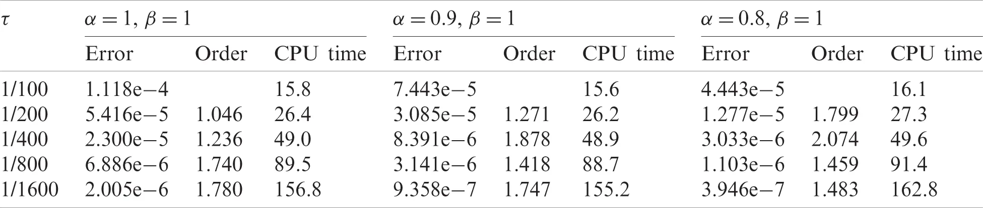
Table 2: The errors, numerical convergence orders in time and CPU times for different temporal step sizes τ with fixed spatial step size Δx=0.01 and fixed time-derivative order α=1
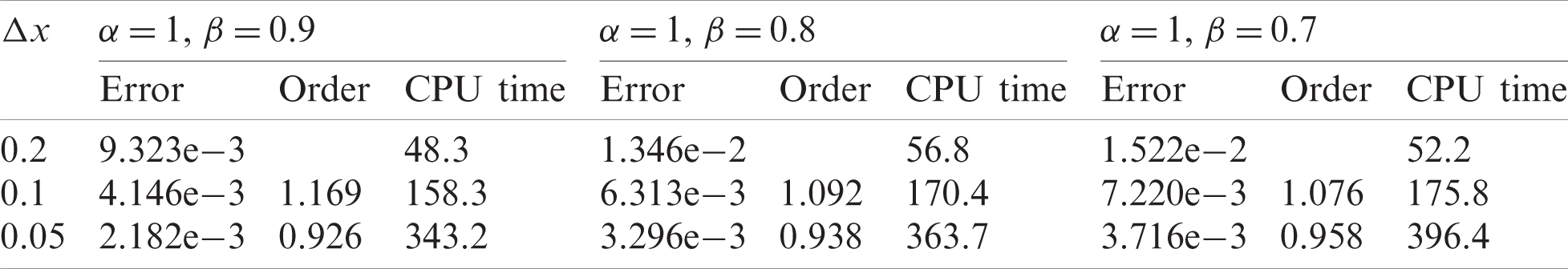
To check the spatial convergence order, we take a sufficiently small temporal step size τ=0.00001 to guarantee that the temporal discretization errors can be neglected compared with the spatial errors. Similar to Tabs. 1 and 2, we record the errors and CPU times calculated under different spatial step sizes in Tabs. 3 and 4. In Tab. 3, the space-derivative order β is fixed to 1 and then forms three different combinations with α. It is observed that the distribution of the spatial convergence order is not uniform in α, and the order decreases dramatically as the spatial step size decreases. In Tab. 4, we set three different combinations of α and β for fixed α=1. It can be noted that the spatial convergence order is very close to 1 regardless of the change in β, which reveals the linear dependency of the scheme error on the spatial step size when β<1. The CPU time under different spatial step sizes does not exhibit a specific growth trend as what we observed in Tabs. 1 and 2. However, considering that the growth rate of the number of discrete spatial grids is the square of the reduction rate of the spatial step size, the CPU time still grows at a slower rate relative to the growth of the number of discrete spatial grids. According to these observations, we can infer that the solver precision can indeed be raised to a certain level at the expense of a relatively small increase in computational complexity (CPU time).
Table 3: The errors, numerical spatial convergence orders and CPU times for different spatial step sizes Δx with fixed temporal step size τ=1e-5 and fixed space-derivative order β=1
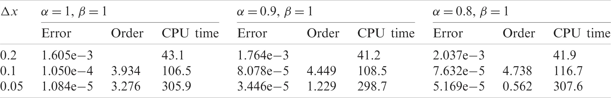
Table 4: The errors, numerical spatial convergence orders and CPU times for different spatial step sizes Δx with fixed temporal step size τ=1e-5 and fixed time-derivative order α=1

Example 5.2 Consider the following steady-state single-carrier transport problem in a 2D p-type organic field effect transistor (OFET).
−Δφ=∇⋅u_=qpεε0(84)
0=−μp∇⋅(u_p)+Dp(∂β+1∂xβ+1+∂β+1∂yβ+1)p+Gp(85)
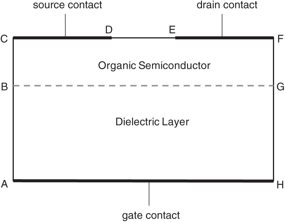
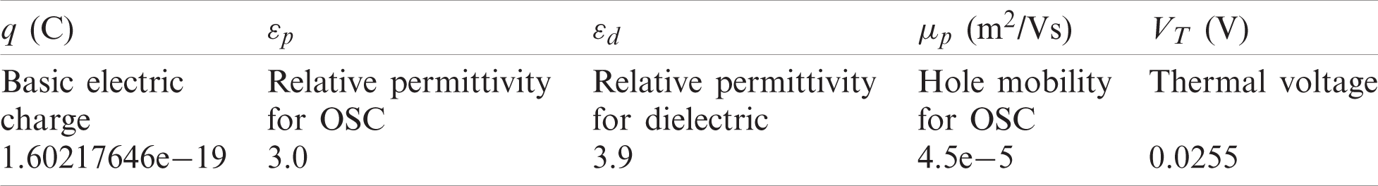
where the effective hole mobility μp and diffusion coefficient Dp are constants for homogeneous materials. The net generation-recombination rate Gp≈0 since the generation and recombination activities are relatively unimportant in OFETs as a majority carrier device [33,37]. The solution domain is defined in Fig. 3, where the size of the organic semiconductor (OSC) layer is 500μm×30nm and the size of the dielectric layer is 500μm×64nm. The parameters for OFET simulation are presented in Tab. 5, and the diffusion coefficient for OSC is determined by Einstein’s relation Dp=VTμp. The geometric sizes and the material types of the OFET domain are the same as the OFET fabricated in [36] and the material parameters are taken from [42,43]. The encapsulating layer (Parylene) in [36] is not considered in this numerical example in order to simplify boundary conditions.

Figure 3: The solution domain of a 2D top-contact bottom-gate (TCBG) OFET device composed of a p-type organic semiconductor layer and a dielectric layer
Table 5: The parameters for OFET simulation

Eqs. (84) and (85) are subject to proper boundary conditions for φ and p. To guarantee the OFET is self-contained, the boundaries AB,BC,DE,FG and GH are constrained by Neumann conditions, i.e., ∂φ∂n=0 and ∂p∂n=0, where n is the unit norm vector to the boundary. Assume that the metal-semiconductor (MS) contacts on CD and EF are ohmic contacts and the barrier voltage is zero, the potentials on CD and EF are specified by φCD=0 and φEF=-1.5 V. Similarly, the boundary potential on AH is specified by φAH=-3.0 V. These electric potential boundary values are all reasonably selected, and the OFET has been proven to work normally under these boundary potentials [36,42]. If we assume the dielectric layer is a perfect isolator, the hole concentration on region ABGH should be 0. The interface between OSC and the dielectric layer (BG) requires the continuity of dielectric displacement, i.e., εp∂φ∂n|BG=εd∂φ∂n|BG. The hole concentrations on MS contacts (i.e., boundaries CD and EF) are assumed to satisfy Dirichlet conditions: pCD=pEF=5e6m-3.
Applying the above boundary conditions and Algorithm 2, we can obtain the simulated steady-state electric potentials and hole concentrations within the solution domain for β=1 and 0.8, as shown in Fig. 4. However, it should be noted that in Example 5.1 and 5.2 only cases where β≥0.7 can be simulated in our program since four generalized (reversed) state transition functions Φ^i(Δx) (i=1,2,3,4) may blow up to infinity as Δx is small and β<0.7. For the cases of β=1 and β=0.8, we impose the specified boundary conditions and obtain the simulated surface plots of electric potentials and hole concentrations in Fig. 4. It is observed that the distribution of electric potentials is not significantly affected by the selection of different β. Nevertheless, the profiles of hole concentration under different β are obviously shifted along the thickness direction, which implies that different β values are related to the intensity of charge carriers’ diffusion motions.
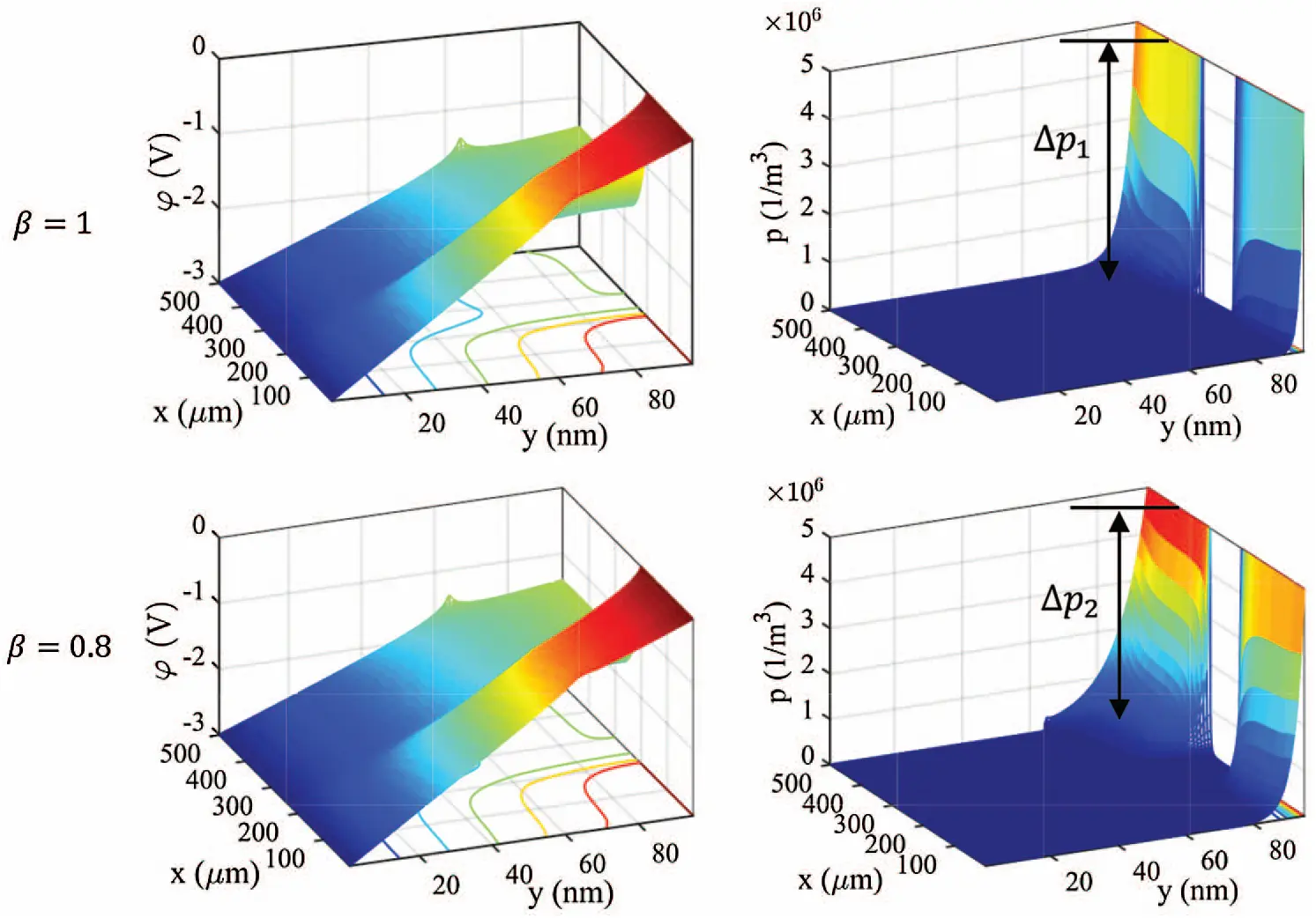
Figure 4: The simulated steady-state electric potentials and hole concentrations within the thinner solution domain for an OFET when space-derivative order β=1 and β=0.8, respectively
The current density contains drift and diffusive components, i.e., J=-qμpp∇φ-qDpC∇rβp, and the diffusive component is proportional to the fractional gradient operator C∇rβp, where C∇rβp=(0CDxβp0CDyβp). We can approximate the fractional derivative by 0CDyβp≈ΔpΔyβ. Since the concentration step changes and the spatial step sizes comply with Δp1>Δp2 and Δy<Δy0.8, we can have 0CDy1p>0CDy0.8p. This result suggests that the charge carriers’ diffusive motions are enhanced for larger β.
Since it is challenging in this example to find an initial value condition consistent with the boundary conditions, even if we can get the steady-state solution for the OFET, it is almost impossible to obtain a transient solution that approaches the steady-state solution over time. To explore the effects of time-derivative order α on the transient dynamics of the organic semiconductor devices, we consider a photo-agitated solar cell model in the next example.
Example 5.3 Consider the following single-carrier transport problem in a 2D p-type solar cell in both time and space for (x,y)∈Ω and t > 0.
−Δφ=∇⋅u_=qpεε0(86)
∂αp∂tα=−μp∇⋅(u_p)+Dp(∂β+1∂xβ+1+∂β+1∂yβ+1)p+p(x,y,0)t−αΓ(1−α)(87)
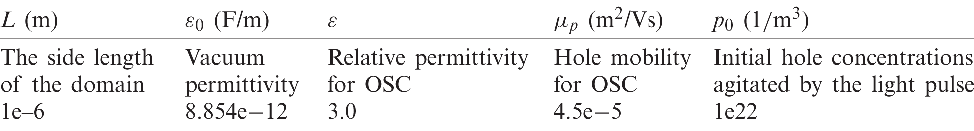
where Ω=(0,L)×(0,L), 0<α≤1, and 0<β≤1. The initial value condition is given by p(x,y,0)=10000p02πLexp(-(x-0.5L)2+(y-0.5L)22×10-8L), and the boundary conditions are specified as p|∂Ω=0, ∂φ∂n|∂Ω=0, where n is the unit normal vector to the boundary surfaces. The other system parameters for this solar cell are presented in Tab. 6. For this example, we intentionally make the kernel radius of the initial hole concentrations much smaller than the side length of the solution domain, i.e., 0.00001L≪L, thus the boundary condition (p|∂Ω=0) is consistent with the initial value condition. This consistency guarantees the solvability of the transient dynamics for the solar cell problem.
Table 6: The parameters for solar cell simulation

In Example 5.3, we let the spatial step size be 1e −8 m and the temporal step size be 1e −6 s. First, we fix β=1 and set α=0.8,0.6 and 0.4 to solve for solutions at t = 1e −5 s. As shown in Fig. 5a, the hole concentration in this setting displays a decaying trend with the decrease of α, while the electric potential remains almost the same for different α. The decay trend in hole concentration can be easily predicted since the hole concentration with smaller α will reduce more within each step of time advancement (i.e., Δp≈Cτα). For the second group of numerical experiments, we fix α=0.9 and set β=1,0.8 and 0.6 to solve for solutions at t = 1e −5 s. It is found in Fig. 5b that the decay rate for hole concentration reduces as the decrease of β, and this phenomenon can be ascribed to the more inactive diffusive motions of charge carriers under smaller β.
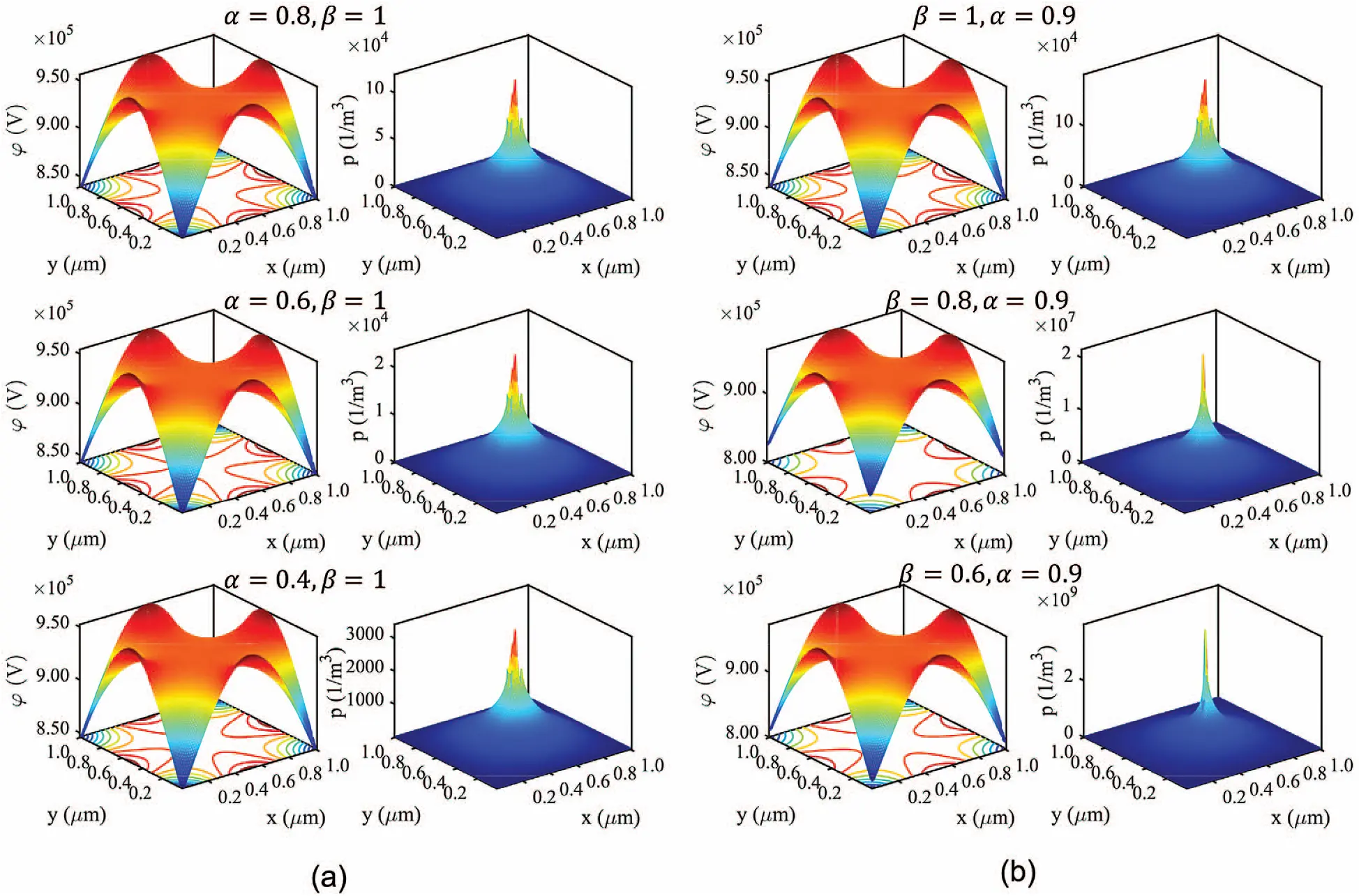
Figure 5: The simulated transient-state electric potentials and hole concentrations within the thinner solution domain for the solar cell when (a) space-derivative order β=1 fixed and α=0.8,0.6 and 0.4, respectively; (b) time-derivative order α=0.9 fixed and β=1,0.8 and 0.6, respectively
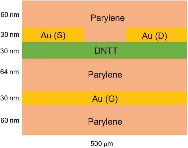
Figure 6: The solution domain of a 2D top-contact bottom-gate (TCBG) OFET device composed of a p-type organic semiconductor layer, a dielectric layer and encapsulating layers (top and bottom)
6 Experimental Validation of the Fractional Drift-Diffusion OFET Model
In Example 5.2, we simplify boundary conditions to better discuss the influence of β values on the charge carriers’ diffusive motions in the steady-state OFET. As an extension to Example 5.2, this section provides the experimental validation for the Fr-DD model. The fabrication and the experimental characterization of the OFET that we model was discussed in [36]. As shown in Fig. 6, compared to the simplified structure of the OFET in Example 5.2, the complete structure of the OFET is encapsulated in a polymer layer made of Parylene and all the metallic electrodes have a thickness of 30 nm. The material parameters are specified in Tab. 5. In addition to the boundary conditions given in Example 5.2, we should also treat the encapsulating layer as a perfect insulator, where no charge carrier is transmitted, and the dielectric displacement should be continuous on its borders.
Consider that the length of the source electrode LS and the drain electrode LD are both 200μm and the width of the OFET (out-of-plane dimension) W is 1000μm, the net current flowing through the drain electrode is evaluated by
Ids=W∫0LDJy(x)dx≈W∑iD=1LD/ΔxJYiD,jD⋅Δx=W∑iD=1LD/Δx(Φ^1(Δy)piD,jD−1−piD,jD)qDpJ0+βΦ^1(Δy)⋅Δx(88)
where Jy is the y-component of the continuous current density at the Au-DNTT interface, iD is the discrete grid index in the x-direction and jD is the discrete grid y index at the Au-DNTT interface. In our case, the spatial step sizes Δx=5μm and Δy=1nm, so we can fix jD = 184 and calculate the summation over iD=1,…,40. The fractional Riemann-Liouville integral J0+βΦ^1(Δy) is then evaluated using Eq. (48).
The β value in the fractional drift diffusion OFET model depends on the spatial coordinates and electrode potentials, i.e., β=B(x,y,Vgs,Vds). This inhomogeneity of β for different spatial coordinates and boundary conditions is caused by the irregular crystalline structure of OSCs and the electronic polarization under different boundary conditions [44,45]. If we ignore the dependence of β on spatial coordinates and only consider its dependence on Vgs and Vds, we can obtain the relationship curves for β=B(Vgs,Vds) in Figs. 7b and 8b by fitting the experimental data.
When β is adjusted for a fixed Vds and varying Vgs according to Fig. 7b, we can utilize Eq. (88) to calculate the drain current Ids under different Vgs and obtain the theoretical transconductance. In Fig. 7a, it is found that the theoretical transconductance curve (solid black line) is in good agreement with the experimentally measured transconductance (red circles). Similarly, if we adjust β for varying Vds and four fixed Vgs according to dependence curves in Fig. 8b, we can notice that the theoretical output curves (black solid lines) can well fit with the experimentally characterized outputs (Symbol, i.e., red circles, blue squares, etc.) as shown in Fig. 8a. These results not only confirm the validity of the Fr-DD model for predicting the OFET characteristics, but also suggest the highly nonlinear dependence of β value on the electrode potentials Vgs and Vds. The relationship curves between β and electrode potentials can be constructed very quickly by writing a simple optimization subroutine to minimize the error between the experimental data and the theoretical predictions. Due to the flexibility of adjusting β, the Fr-DD model avoids considering the involuted trap states in OSCs, thus greatly improving the modeling efficiency of OSC devices compared with the conventional OFET analytic models involving the trap or impurity states.
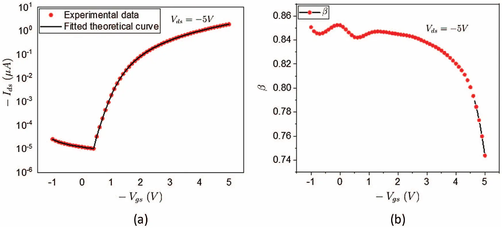
Figure 7: (a) The experimentally measured transconductance at a fixed Vds = −5 V compared with the fitted theoretical transconductance curve obtained from the fractional drift diffusion model; (b) The adjusted β values at different Vgs and a fixed Vds = −5 V
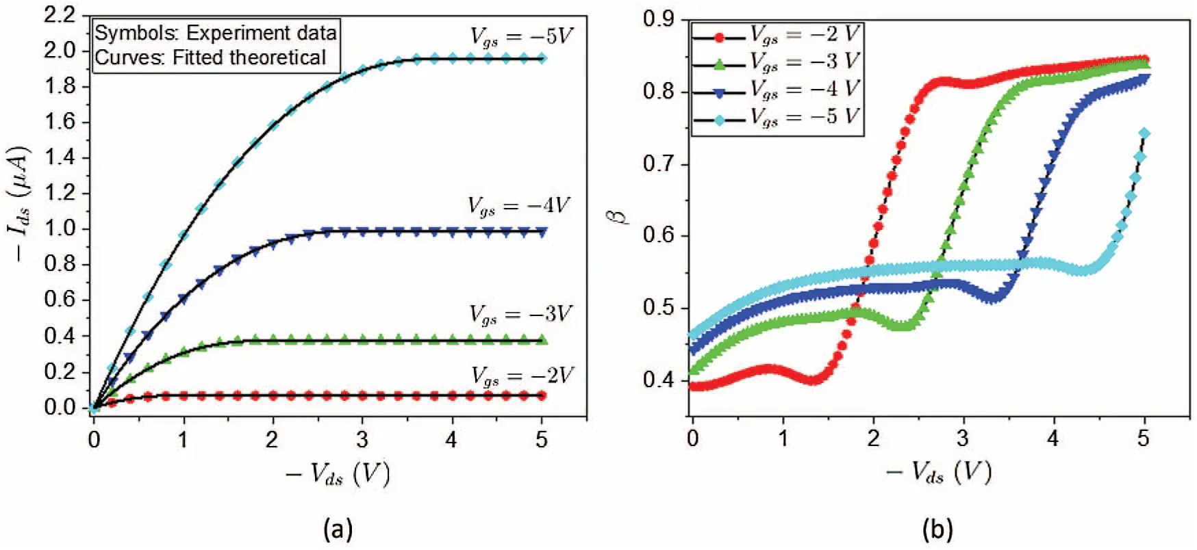
Figure 8: (a) The experimentally measured output curve at a series of fixed Vgs=-5~-2 V compared with the fitted theoretical output curve obtained from the fractional drift diffusion model; (b) The adjusted β values at different Vds and a series of fixed Vgs=-5~-2 V
7 Conclusion
This work aimed to develop a Fr-DD model solver for simulating the anomalous dynamics of OSC devices. Two algorithms based on a novel discretization scheme and successively over-relaxed Gummel’s iteration are proposed here to solve the transient and steady-state Fr-DD model equations. This study has identified the consistency of the two algorithms by showing that the truncation error from the discretized divergence of current density functions will vanish with the spatial step size to a positive fractional order of 1-β. The convergence analysis reveals that the Gummel mapping is a contraction mapping if we consider the successive over-relaxation mechanism in the Gummel’s iteration, which thus completes the proof of convergence. Three numerical examples, including one benchmark example and two others constructed from the perspective of engineering applications are employed to demonstrate the algorithms’ accuracy and computational performance. It is found in the first example that altering α and β can impact the spatial convergence order but only varying α will affect the convergence order in time. The increase rate of CPU time is less than the shrinking rate of temporal step size and lower than the growth rate of spatial grid points. These findings suggest that our solver has high precision and fast computational speed as it limits the computational error to a predefined satisfactory level (from ~10-4 to ~10-6) at a relatively small expense of CPU time (from ~20 s to ~100 s). The results reported in two numerical examples reveal the prediction and characterization of the transient-state and steady-state dynamics for any type of organic semiconductor device. Finally, we provide experimental verification for the fractional drift diffusion model of a DNTT-OFET. We stipulate that this is the first to date exploration of the Fr-DD model solver laying the groundwork for future research into fractional drift diffusion modeling of flexible organic electronics.
Funding Statement: This work was supported in part by the National Science Foundation through Grant CNS-1726865 and by the USDA under Grant 2019-67021-28990.
Conflicts of Interest: The authors declare that they have no conflicts of interest to report regarding the present study.
1This was initially a simplified Fr-DD model with only time-derivative fractionalized, the order of spatial derivatives remained integer.
References
1. R. E. Bank, D. J. Rose and W. Fichtner, “Numerical methods for semiconductor device simulation,” IEEE Transactions on Electron Devices, vol. 30, no. 9, pp. 1031–1041, 1983. [Google Scholar]
2. E. Gartland, “On the uniform convergence of the Scharfetter–Gummel discretization in one dimension,” SIAM Journal on Numerical Analysis, vol. 30, no. 3, pp. 749–758, 1993. [Google Scholar]
3. B. Lu and Y. C. Zhou, “Poisson–Nernst–Planck equations for simulating biomolecular diffusion-reaction processes II: Size effects on ionic distributions and diffusion-reaction rates,” Biophysical Journal, vol. 100, no. 10, pp. 2475–2485, 2011. [Google Scholar]
4. Q. Zheng, D. Chen and G. W. Wei, “Second-order Poisson Nernst–Planck solver for ion channel transport,” Journal of Computational Physics, vol. 230, no. 13, pp. 5239–5262, 2011. [Google Scholar]
5. J. Pods, J. Schönke and P. Bastian, “Electrodiffusion models of neurons and extracellular space using the Poisson–Nernst–Planck equations-Numerical simulation of the intra-and extracellular potential for an axon model,” Biophysical Journal, vol. 105, no. 1, pp. 242–254, 2013. [Google Scholar]
6. D. S. Bolintineanu, A. Sayyed-Ahmad, H. T. Davis and Y. N. Kaznessis, “Poisson–Nernst–Planck models of nonequilibrium ion electrodiffusion through a protegrin transmembrane pore,” PLoS Computational Biology, vol. 5, no. 1, pp. e1000277, 2009. [Google Scholar]
7. W. Van Roosbroeck, “Theory of the flow of electrons and holes in germanium and other semiconductors,” Bell System Technical Journal, vol. 29, no. 4, pp. 560–607, 1950. [Google Scholar]
8. R. F. Pierret, Semiconductor Device Fundamentals. Boston, MA, USA: Addison-Wesley, 1996. [Google Scholar]
9. G. L. Tan, X. L. Yuan, Q. M. Zhang, W. H. Ku and A. J. Shey, “Two-dimensional semiconductor device analysis based on new finite-element discretization employing the S-G scheme,” IEEE Transactions on Computer-Aided Design of Integrated Circuits and System, vol. 8, no. 5, pp. 468–478, 1989. [Google Scholar]
10. Y. Yuan, “Finite difference fractional step methods for the transient behavior of a semiconductor device,” Acta Mathematica Scientia, vol. 25, no. 3, pp. 427–438, 2005. [Google Scholar]
11. Y. Yuan, Q. Yang, C. Li and T. Sun, “Numerical method of mixed finite volume-modified upwind fractional step difference for three-dimensional semiconductor device transient behavior problems,” Acta Mathematica Scientia, vol. 37, no. 1, pp. 259–279, 2017. [Google Scholar]
12. Y. Li, “A two-dimensional thin-film transistor simulation using adaptive computing technique,” Applied Mathematics and Computation, vol. 184, no. 1 SPEC. ISS., pp. 73–85, 2007. [Google Scholar]
13. R. C. Chen and J. L. Liu, “Monotone iterative methods for the adaptive finite element solution of semiconductor equations,” Journal of Computational and Applied Mathematics, vol. 159, no. 2, pp. 341–364, 2003. [Google Scholar]
14. J. W. Jerome, Analysis of Charge Transport. Berlin, Germany: Springer-Verlag, 1996. [Google Scholar]
15. J. W. Jerome and T. Kerkhoven, “Finite element approximation theory for the drift diffusion semiconductor model,” SIAM Journal on Numerical Analysis, vol. 28, no. 2, pp. 403–422, 1991. [Google Scholar]
16. J. W. Jerome, “Consistency of semiconductor modeling: An existence/stability analysis for the stationary Van Roosbroeck system,” SIAM Journal on Applied Mathematics, vol. 45, no. 4, pp. 565–590, 1985. [Google Scholar]
17. T. Kerkhoven, “On the effectiveness of Gummel’s method,” SIAM Journal on Scientific and Statistical Computing, vol. 9, no. 1, pp. 48–60, 1988. [Google Scholar]
18. R. T. Sibatov and V. V. Uchaikin, “Fractional differential approach to dispersive transport in semiconductors,” Physics-Uspekhi, vol. 52, no. 10, pp. 1019–1043, 2009. [Google Scholar]
19. R. Tsekov, “Brownian motion of a classical particle in quantum environment,” Physics Letters, Section A: General, Atomic and Solid State Physics, vol. 382, no. 33, pp. 2230–2232, 2018. [Google Scholar]
20. K. Y. Choo, S. V. Muniandy, K. L. Woon, M. T. Gan and D. S. Ong, “Modeling anomalous charge carrier transport in disordered organic semiconductors using the fractional drift-diffusion equation,” Organic Electronics, vol. 41, pp. 157–165, 2017. [Google Scholar]
21. J. Kniepert, M. Schubert, J. C. Blakesley and D. Neher, “Photogeneration and recombination in P3HT/PCBM solar cells probed by time-delayed collection field experiments,” The Journal of Physical Chemistry Letters, vol. 2, no. 7, pp. 700–705, 2011. [Google Scholar]
22. A. J. Mozer, G. Dennler, N. S. Sariciftci, M. Westerling, A. Pivrikas et al., “Time-dependent mobility and recombination of the photoinduced charge carriers in conjugated polymer/fullerene bulk heterojunction solar cells,” Physical Review B: Condensed Matter and Materials Physics, vol. 72, no. 3, pp. 35217, 2005. [Google Scholar]
23. H. Scher and E. W. Montroll, “Anomalous transit-time dispersion in amorphous solids,” Physical Review B: Condensed Matter and Materials Physics, vol. 12, no. 6, pp. 2455–2477, 1975. [Google Scholar]
24. J. Orenstein and M. Kastner, “Photocurrent transient spectroscopy: Measurement of the density of localized states in a -As2Se3,” Physical Review Letter, vol. 46, no. 21, pp. 1421–1424, 1981. [Google Scholar]
25. T. Tiedje and A. Rose, “A physical interpretation of dispersive transport in disordered semiconductors,” Solid State Communications, vol. 37, no. 1, pp. 49–52, 1981. [Google Scholar]
26. H. Antoniadis and E. A. Schiff, “Unraveling the μτ-mystery in a-Si:H,” Journal of Non-Crystalline Solids, vol. 138, no. PART 1, pp. 435–438, 1991. [Google Scholar]
27. A. H. A. El Ela and H. H. Afifi, “Hopping transport in organic semiconductor system,” Journal of Physics and Chemistry of Solids, vol. 40, no. 4, pp. 257–259, 1979. [Google Scholar]
28. C. Liu, K. Huang, W. T. Park, M. Li, T. Yang et al., “A unified understanding of charge transport in organic semiconductors: The importance of attenuated delocalization for the carriers,” Materials Horizons, vol. 4, no. 4, pp. 608–618, 2017. [Google Scholar]
29. T. Upreti, Y. Wang, H. Zhang, D. Scheunemann, F. Gao et al., “Experimentally validated hopping-transport model for energetically disordered organic semiconductors,” Physical Review Applied, vol. 12, no. 6, pp. 64039, 2019. [Google Scholar]
30. R. T. Sibatov and V. V. Uchaikin, “Fractional differential kinetics of charge transport in unordered semiconductors,” Semiconductors, vol. 41, no. 3, pp. 335–340, 2007. [Google Scholar]
31. K. Y. Choo and S. V. Muniandy, “Fractional dispersive transport in inhomogeneous organic semiconductors,” International Journal of Modern Physics: Conference Series, vol. 36, pp. 1560008, 2015. [Google Scholar]
32. A. Alaria, A. M. Khan, D. L. Suthar and D. Kumar, “Application of fractional operators in modelling for charge carrier transport in amorphous semiconductor with multiple trapping,” International Journal of Applied and Computational Mathematics, vol. 5, no. 6, pp. 167, 2019. [Google Scholar]
33. A. Dev Dhar Dwivedi, S. Kumar Jain, R. Dhar Dwivedi and S. Dadhich, “Numerical simulation and compact modeling of thin film transistors for future flexible electronics,” in Hybrid Nanomaterials-Flexible Electronics Materials, 1st ed., vol. 1. London, UK: IntechOpen, 2020. [Google Scholar]
34. I. Podlubny, Fractional Differential Equations. San Diego, CA, USA: Academic Press, 1999. [Google Scholar]
35. Y. Yang and H. H. Zhang, Fractional Calculus with Its Applications in Engineering and Technology, 1st ed., vol. 3. San Rafael, CA, USA: Morgan & Claypool Publishers LLC, 2019. [Google Scholar]
36. R. A. Nawrocki, N. Matsuhisa, T. Yokota and T. Someya, “300-nm imperceptible, ultraflexible, and biocompatible e-skin fit with tactile sensors and organic transistors,” Advanced Electronic Materials, vol. 2, no. 4, pp. 1500452, 2016. [Google Scholar]
37. H. J. Haubold, A. M. Mathai and R. K. Saxena, “Mittag-leffler functions and their applications,” Journal of Applied Mathematics, vol. 2011, no. 3, pp. 1–51, 2011. [Google Scholar]
38. C. Li, D. Qian and Y. Chen, “On Riemann–Liouville and Caputo derivatives,” Discrete Dynamics in Nature and Society, vol. 2011, pp. 1–15, 2011. [Google Scholar]
39. T. Blaszczyk, J. Siedlecki and M. Ciesielski, “Numerical algorithms for approximation of fractional integral operators based on quadratic interpolation,” Mathematical Methods in the Applied Sciences, vol. 41, no. 9, pp. 3345–3355, 2018. [Google Scholar]
40. P. Moin, Fundamentals of Engineering Numerical Analysis, 2nd ed., vol. 1. Cambridge, UK: Cambridge University Press, 2010. [Google Scholar]
41. P. J. Roache, “Code verification by the method of manufactured solutions,” Journal of Fluids Engineering, Transactions of the ASME, vol. 124, no. 1, pp. 4–10, 2002. [Google Scholar]
42. Y. Yang, R. A. Nawrocki, R. M. Voyles and H. H. Zhang, “Modeling of the electrical characteristics of an organic field effect transistor in presence of the bending effects,” Organic Electronics, vol. 88, pp. 106000, 2021. [Google Scholar]
43. Y. Yang, R. Nawrocki, R. Voyles and H. H. Zhang, “Modeling of an internal stress and strain distribution of an inverted staggered thin-film transistor based on two-dimensional mass-spring-damper structure,” Computer Modeling in Engineering & Sciences, vol. 125, no. 2, pp. 515–539, 2020. [Google Scholar]
44. E. F. Valeev, V. Coropceanu, D. A. Da Silva Filho, S. Salman and J. L. Brédas, “Effect of electronic polarization on charge-transport parameters in molecular organic semiconductors,” Journal of the American Chemical Society, vol. 128, no. 30, pp. 9882–9886, 2006. [Google Scholar]
45. S. Erker and O. T. Hofmann, “Fractional and integer charge transfer at semiconductor/organic interfaces: The role of hybridization and metallicity,” The Journal of Physical Chemistry Letters, vol. 10, no. 4, pp. 848–854, 2019. [Google Scholar]