Computers, Materials & Continua DOI:10.32604/cmc.2021.017653
Article

Time and Quantity Based Hybrid Consolidation Algorithms for Reduced Cost Products Delivery

Muhammad Ali Memon1, Asadullah Shaikh2,*, Adel Sulaiman2, Abdullah Alghamdi2, Mesfer Alrizq2 and Bernard Archimède3

1Department of Information Technology, University of Sindh, Jamshoro, Sindh, 76090, Pakistan
2College of Computer Science and Information Systems, Najran University, Najran, 61441, Saudi Arabia
3University of Toulouse, INP-ENIT, 47 Avenue d’Azereix, BP1629, F-65016, Tarbes Cedex, France
*Corresponding Author: Asadullah Shaikh. Email: asshaikh@nu.edu.sa
Received: 06 February 2021; Accepted: 25 March 2021

Abstract: In today’s competitive business environment, the cost of a product is one of the most important considerations for its sale. Businesses are heavily involved in research strategies to minimize the cost of elements that can impact on the final price of the product. Logistics is one such factor. Numerous products arrive from diverse locations to consumers in today’s digital era of online businesses. Clearly, the logistics sector faces several dilemmas from order attributes to environmental changes in this regard. This has specially been noted during the ongoing Covid-19 pandemic where the demands on online businesses have increased several fold. Consequently, the methodology to optimise delivery cost and its impact on environmental focus by reducing CO2 emissions has gained relevance. The resultant strategy of Shipment Consolidation that has evolved is an approach that combines one or more transport orders in the same vehicle for delivery. Shipment Consolidation has been categorized in three order scheduling approaches: Time based consolidation, Quantity based consolidation, and a Hybrid (Time-Quantity) based consolidation. In this paper, a new Hybrid Consolidation approach is presented. Using the Hybrid approach, it has been shown that order delivery can be facilitated by taking into account not only the order pick up time, but also the total order quantity. These results have shown that if a time window is available in respect of the order delivery time, then the order can be delayed from pickup to consolidate it with other orders for cost optimization. This hybrid approach is based on four consolidation principles, two of which work on fixed departure and two, on demand departure. Three of these rules have been implemented and tested here with an application case study. Statistical analysis of the results is illustrated with different planning evaluation indicators. The Result analyses indicate that consolidation of orders is increased with each implemented rule hence motivating us towards the implementation of the fourth rule. Testing with bigger data sets is required.

Keywords: Consolidation; transportation; supply chain; cost minimization

1  Introduction

Due to the economic globalization in recent times, increasing changes in production and distribution activities have been found to strain the natural ecosystem. As a result, important environmental issues are becoming more and more evident, requiring attention from both business and research communities. Accordingly, the industrial sector needs to make every effort to use resources efficiently to cope with the demands for sustainability.

Consequently, greening the supply chain is becoming a significant challenge for businesses. This involves the designing of supply chain operations including product design, material selection and sourcing, optimizing manufacturing processes and ensuring delivery of the final product to the consumers [1]. The efficient use of logistics plays a significant role in greening the supply chain. Transportation is recognized as a major environmental hazard as vehicles not only emit CO2 and other harmful gases but are also a major cause of noise pollution.

Previous research has underlined that the timing and size of the shipment are important for the better responsiveness of the supply chain [2–4]. Nevertheless, recurrent individual shipments from supplier to buyer minimize inventory keeping but proportionally increases transportation costs. To counter this, the vendor is required to ship larger quantities of goods which understandably leads to a large inventory to reduce the number of shipments. Consequently, it is not necessary to maintain a one-to-one link between the vendor and the supplier. Hence if vendors are situated nearby, their shipments can share a common route for delivery. This can reflect as an advantage if a single consolidated transport vehicle can deliver goods from several vendors to several suppliers.

Several aspects of economic and environmental issues can benefit from Shipment Consolidation (SCL). This ranges from cost reduction per unit, per shipment, or per unit volume to minimize transport travels, road occupancy, petrol usage and noise pollution, etc. For example, the benefit of applying consolidation in petroleum product sales result in transportation costs savings of almost $1 million annually [5]. As an example, the Kelloggs Company saves approximately US $35 million per year in inventory and distribution costs by applying consolidation [6].

SCL will aid in greening the supply chain to reduce costs as well as pollution, which is becoming a major concern of highly polluted large cities like Beijing, New York, Karachi, etc.

SCL is an environmentally responsible transportation strategy that groups two or more transport orders to dispatch a large quantity of goods in the same vehicle to the same (or close) customer area [7]. SCL can empower cost reduction by functioning with both Full-Truckload (FTL) and Less-Than-TruckLoad (LTL). For FTL, the transportation vehicle is required to pick up a shipment from one location and deliver it to the other, whereas in LTL the shipper reserves and pays for part of the vehicle’s space, the vehicle is required to do more pickups and deliver goods to multiple locations.

There are three categories of problems in SCL. The first is a quantity-based policy that determines the maximum quantity that can be consolidated for a shipment [8]. The second is a time-based policy, in which the vehicle has to wait for consolidated order for a certain time [9,10]. The third is a hybrid time and quantity policy which is the combination of the two [11].

In this paper, we propose a hybrid time and quantity policy for different consolidation rules in which vehicles have fixed routing routes with fixed and flexible dates of departures. A genericity of these rules is presented.

The rest of this paper is structured as follows. Section 2 presents related work. Section 3 focuses on the formalism that will be used in the scheduling algorithm and Section 4 explores the steps of the scheduling algorithm. Section 5 presents the consolidation rules. Section 6 describes the test case scenario. Section 7 analyses the experimental results. Section 8 provides conclusions and future directions.

2  Related Work

A review of the literature reveals that SCL has been studied for many years. In the eighties, many research works dealt with the economic interest of SCL. Blumenfeld et al. [12] compared the cost and size of transports and inventories in direct shipping or shipping via terminals. Carlos Daganzo established that the costs (and thus the interest) of using transhipment terminals depend on the number of pick-up and delivery locations (one-to-many, many-to-one or many-to-many) [13,14]. Randolph Hall investigated different ways of optimizing SCL according to the number of transhipment terminals and the length of travels [15] and the frequency and length of rounds [16]. Lately, there has been a reinvigoration of interest in SCL because of the environmental concerns raised. This signifies that Greening the Supply Chain can result in reducing CO2 emissions, simply by consolidating shipments [17]. SCL does not only reduce environmental impact but also reduces transportation costs [18,19]. A coordinated approach is proposed for the delivery of semi-finished and finished products to a small number of customers [20]. In terms of operational costs and reduction of vehicle used, both cost reduction of almost 35-40% and vehicle usage of approximately 33% is attained [21]. Vehicle sharing achieves a total reduction of 10% in costs in SCL [22]. Ma et al. [23] focus on the reduction of carbon emissions through container shipment consolidation and optimization. Wei et al. [24] and Hanbazazah et al. [25] propose the method for dynamic order fulfillment with delivery deadlines and expedited shipping options for reasonable prices.

Three types of strategies have been identified to perform the transport of several shipments [26,14,27,28].

—Direct transport strategy without consolidation, involving multiple travels, but no transhipment. This strategy is economically interesting in the case of one-to-many or many-to-one distribution.

—Peddling strategy, where freight is consolidated according to pick-up locations close to each other and/or destinations close to each other. SCL can then be called spatial.

—Hub-and-spoke strategy, where freight is consolidated to be transported from one terminal to another. In this case, SCL is known as temporal.

A study on the economic impact of FCC (Freight Consolidation Centres) and their localization around cities has been explained in [29], showing that these kinds of terminals can decrease the number of transports, and thereby costs and CO2 emissions. A multi-agents system that aims to choose the best transport strategy amongst these three for a 3PL company according to parameters such as terminal localization or waiting time has been described in [30]. Nevertheless, this kind of system does not take into account cooperation between 3PL companies to perform a long or complicated travel.

Peddling or hub-and-spoke strategies both imply setting up the Economic Order Quantity (EOQ) for production and transport while taking into account the costs of production, inventory and transport facilities [31,32,19]. An SCL policy needs parameters to be set [33]. Three SCL policies have been described in the literature [26,28,34], (1) time-based policy, (2) quantity-based policy and (3) hybrid time-and-quantity-based policy. These policies have been widely addressed, especially to optimize the different thresholds that are needed. Gupta et al. proposed a decision support system to determine the load threshold according to time and transhipment and transportation costs [8]. Probabilistic modeling and simulation are performed to decide the maximum waiting time and desired product quantity [35]. The Renewal theory was used to determine the time elapsed or the load reached before dispatch [36]. Few studies address the problem of choosing which freight should be shipped and which freight should wait for the next transport. The impact of different priority rules on the overall performance of transportation planning has seldom been addressed. In our work, orders are sorted based on rules like First In First Out (FIFO) and Margin.

3  Problem Formalization

In order to present the rules, it is firstly important to formalize the problem by defining different terminologies used within the shipment rules.

3.1 Transport Resource

Transport resource (Vehicle) definition comprises of two types of parameters fixed and variable. Fixed parameters consist of (1) Resource representing the vehicle, (2) Location representing pickup location, (3) Capacity representing vehicle's carrying capacity of products and (4) Activity representing a direct (no stop) travel which forms a predefined route for the vehicle. Variable parameters consist of Availability representing its accessibility for travel, Duration represents the active hours for the transport being used, Maximum Wait Time (MWT) that a vehicle can wait. The activity completion time is represented by the variable Co-efficient. Its value may change during travel and if a vehicle is set to complete its transit within stipulated time then it is set to one. If a vehicle is lethargic, it may get delayed so the coefficient will change, for example, if Coeff is set to 1.5 then the transit time will increase by an additional 50%. Finally, the schedule represents the dates of travel for the vehicles. V={vj/j=1,…,nv} where V represents the set of all vehicles (transport resources).

CDj:CDj be the current date including the time of the vehicle vj.

LoadRj(x): LoadRj(x) Represents the residing load that vehicle is holding at date x and x can be CDj.

Capj: parameter Capj be the total capacity of the vehicle vj∈V.

3.2 Activity

Activity is part of the delivery order. It is a nonstop continuous transit of a vehicle on a route or a section of a route, from the loading site to the offloading site, which can be the origin or destination points as well as in between segments.

A={ai/i=1,…,n}: A represents the group of activities that vehicle vj∈V can perform.

Dur:A⟶R: Dur(ai) define the duration of the activity ai∈A.

Delivery order: O={(OBu,PTu,PLu,DLu,PTu,DTu,PQu)/u=1,…,no}: O is the group of all delivery orders, where OBu the objective is, PTu is the product type, PLu is the pickup position, DLu is the delivery position, PTu is the pickup time, DTu is the delivery time and PQu is the product quantity of the order.

3.3 Task

A task is a demand for the execution of an activity. One task can only be linked to a single activity, but there could be many tasks demanding the execution of the same activity.

T={tu,c/u=1,…,no∈O,c=1,…,ntu}: T is the group of all tasks of all the delivery orders and c represents the corresponding number of the task for the delivery order u.

ta:T⟶A ta(t)=a∈A: Function ta(t) associate for each demanded task t∈T the basic activity in A.

at={tu,c∈T,∀∈O,∀c=1,…,ntu/ta(tu,c)=a}: Function at associate for each task the basic activity a∈A for the set of associated tasks in T.

Vtu,i={vb∈V,b=1,…,nvtu,i/ta(tu,i)∈V}: Vtu,i is the group of vehicles that can execute the task tu,i∈T.

Tj={t1,t2,…,tq∈T/ta(tu)=ai,∀u=1,…,q}: Tj is the group of all of the tasks for the activity ai.

3.4 Transport Network

Transport network TN(N,E) is the directed graph consisting of nodes and arcs E. It is constituted by joining all the activities for the vehicles. Each link in the network is an activity. A node is termed as pickup place or delivery place, from or where products can be picked up or delivered. Each node in the network has particular coordinates of xi, and yi, making it a geographical location on the map. Each arc Ei∈E has a standard time for traveling. Nevertheless, the total time for traveling a particular arc is not fixed but depends on the vehicle's coefficient and load that vehicle is carrying.

3.5 Routing

Delivery orders arriving from customers consist of pickup and delivery places of the shipment. Between pickup and delivery places, in the transport network, there are several arcs possible, where each arc is the corresponding basic activity, and each activity is performed by a single or more than one vehicle. Hence, taking into account the transportation network, vehicles that can execute the activity for the requested delivery order, a route is constructed. This consists of a set of sequential activities necessary for the delivery of an order. Regarding this, some tasks correspond to activities performed by transport vehicles. This routing is achieved through an autonomous tool for route finding called Path Finder agent [37].

DOu={tu,k∈T/k=1,…,ntu}: TOu is the order of tasks between PLu and DLu for the delivery order, u constituted according to the activities that can be executed by the fleet of vehicle logistics providers.

4  Scheduling Algorithm

Delivery order as explained previously is decomposed into several basic activities and each activity can be performed by different vehicles, whichever fits best with the objective function of the delivery order. Hence, there are two possibilities to schedule the delivery of transporter orders. One way is to schedule all the activities at the same time and the second to schedule the activities in incremental order. Here, the authors consider the incremental scheduling of activities. For this purpose, an auction scheduling algorithm is based on the work proposed by B.Archimed [38]. In this algorithm, the order agent and customer agent make the auction environment to schedule the planning. Here, the order agent will represent an order; and the vehicle agent will represent the customer agent. An Agent is an intelligent piece of software that interacts according to the environment in which it is being used.

The Order agent proposes the desired date and time for each activity for the delivery. Similarly, the Vehicle agent representing each vehicle proposes the PP (Potential Position) as the potential date and EP (Effective Position) as the effective date. There is a cycle of scheduling, consisting of three phases. This cycle is repeated until the scheduling of all the tasks is finished incrementally.

4.1 Scheduling Step One

The auction process starts to seek the best possible Potential Position (PP) and Effective Position (EP). In the auction, the order agent representing the delivery order proposes its Wished Position (WP). The process of auction is depicted in Fig. 1. Each order agent plans delivery time for a sequence of tasks corresponding to its delivery order at the earliest considering the idle situation. This earliest delivery time is termed as WP, the desired delivery date for each sequenced task of the delivery order. WP comprises three parameters: (1) Demanded Activity, (2) Wished Start Date (WSD), and Wished End Date (WED), (3) the product type to be delivered. WSD is the earliest pickup time for the order and WED is the WSD+ traveling time of the activity. Traveling time is the estimated or standard time in kilometers determined through any map application.

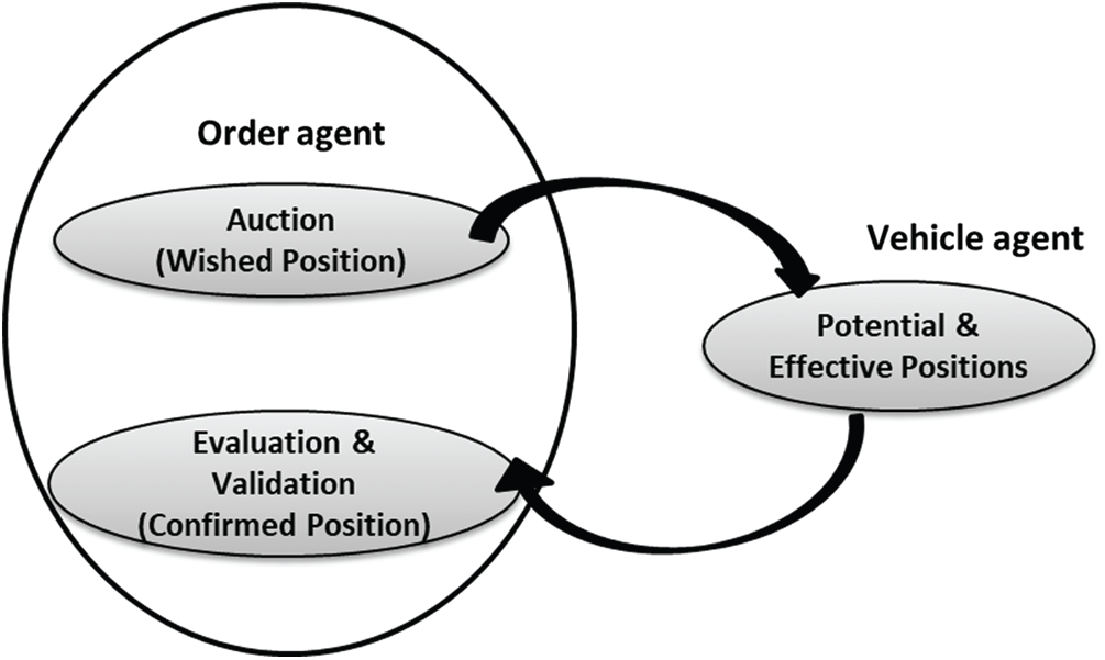
Figure 1: Auction cycle between order and vehicle agent

4.2 Scheduling Step Two

In this step, vehicle agents representing the transport resource (each vehicle) respond to the demand of the order agents in the auction by proposing the Potential and Effective Positions (PP and EP). When all order agents are completed with the planning of tasks with their WP(s). Vehicle agents retrieve that information about the tasks and each vehicle agent chooses the task(s) associated with their corresponding activity. Each vehicle determines the cost of the task’s realization, by calculating the duration of the task which is equal to its coefficient of speed * standard traveling duration of the activity, while total cost is equal to duration determined * cost ratio. All tasks are then arranged in the sorted list according to the priority, where priority is the earliest delivery date of the task and a schedule is proposed for each task at the earliest considering vehicle’s capacity. Hence vehicle pickup date and delivery date are determined for each task picked up from the priority list. A vehicle agent then bids two dates, potential and effective called Potential Position (PP) and Effective Position (EP). PP is scheduled and proposed by taking into account one task at a moment by vehicle agent and EP is scheduled and proposed by considering all the tasks at a moment. EP and PP are depicted in Figs. 2a and 2b respectively.

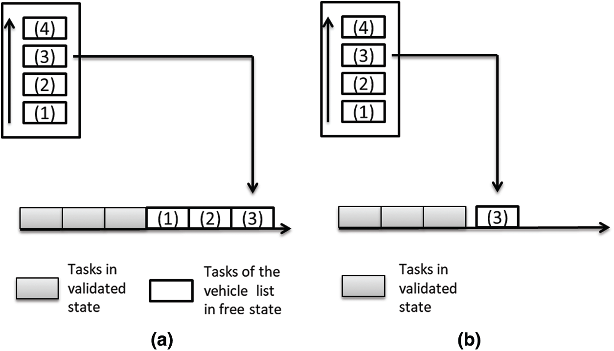
Figure 2: PP and EP planning (a) Planning of effective position (b) Planning of potential position

Consequently for each task, corresponding to its demanded Wished Position (WP), vehicle agents proposes a Potential Position consisting of PP (Potential Start Date (PSD) & Potential End Date (PED)) and Effective Position PP (Potential Start Date (PSD) & Potential End Date (PED)). When all vehicle agents performed planning their PP and EP for their corresponding tasks, they write them back in the environment for order agents to respond.

PPji: PPji is the potential position for ti∈Tj proposed by the vehicle vj where PPji=(PSDji,PEDji) while PSDji and PEDji are the potential start date and potential end date respectively.

EPji: EPji be the effective position for ti∈Tj proposed by the vehicle vj where EPji=(ESDji,EEDji) while ESDji and EEDji are the effective start date and effective end date respectively.

4.3 Scheduling Step Three

In this step, order agents evaluate and validate the position bid by the vehicle agents. Each order reads the corresponding positions from the environment. It starts evaluating each PP and EP in order to seek the best position bid by vehicle agents. This evaluation involves finding out those positions which best meet the objective, set for the delivery order. The objective may be set as an early delivery or less costly delivery or both with the priority on any from them [39]. Subsequently, the validation process starts for both PP and EP.

In the validation process, selected PP and EP are compared directly with WP that was proposed at the start of the auction to decide that task can be validated or is it better to wait for better PP and EP. If the order agent believes that PP and EP can be improved further, then the order agent goes for another cycle of the auction. Subsequently, the new auction cycle starts otherwise if the order agent believes that PP and EP cannot be improved further and therefore, it validates the currently proposed PP and EP. The comparison of position according to the following conditions is given below:

Auction:

—Wished Start Date (WSD)

—Wished End Date (WED)

Best effective position:

—Effective Start Date (ESD)

—Effective End Date (EED)

Best potential position:

—Potential Start Date (PSD)

—Potential End Date (PED)

The validation step is given in the following Fig. 3

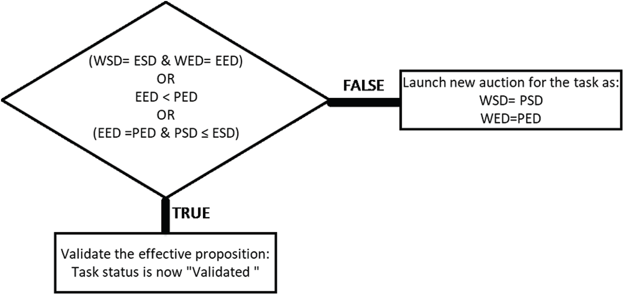
Figure 3: Algorithm for the validation for the task by order agent

An order agent may validate the position by vehicle agent if EP is the same as WP. The negotiation is then stopped for that particular task, and its state is updated from “Free” to “Validated.” Order agent may also validate the position if PP and EP are both identical or the same. Therefore, the order agent has no other option but to choose these PP and EP and validate. Though, if EP is not the same as WP and PP are better than EP, means PP is close to WP. Hence the order agent will take a risk considering that EP will become the same as PP in the next coming cycles. Consequently, a new cycle of the auction is commenced for this task by updating WP to PP, hoping to find the best EP and state of the task remains unchanged means “Free.”

The ultimate goal of the auction process is to choose those vehicles that provide a better solution in achieving the objective keeping in view the time constraints. The solution achieved through the auction process may be a little time consuming or quite slow, as there is a possibility that only a single task can be validated in one cycle. Considering this limitation, another solution is the global validation with a larger view is considered in making decisions [39].

After all the order agents have validated their positions, an agreement is made with vehicles, that are selected for the execution of the tasks. Status of the validated tasks is then updated to “confirmed" state and each task has now confirmed the position that is to say (Confirmed Start Sate and (CSD) and Confirmed End Date (CED)). Once a task is confirmed, it cannot be altered. The auction cycle is repeated until all the tasks are updated and confirmed or there is no more WP left for any task. This marks the end of the scheduling process.

5  Shipment Consolidation Rules

5.1 Rules Formalization

In the shipment consolidation problem, two types of transport modes for the vehicles are considered, i.e., when a vehicle has a Fixed departure schedule and Demand responsive departure. In a Fixed departure mode, the transport runs according to a schedule, where timing and order are fixed for an activity, for example, cargo moving through buses and trains. In a Demand responsive case, the transport waits for orders and their departures are scheduled dynamically.

Also, two important priority lists are used for shipment consolidation: WSD and the Margin. The WSD is used by the vehicle agent to list tasks in increasing order of their date of wish to start a task. So, a task with an earlier pickup time is handled earlier than other tasks and the delayed tasks will be added to the priority list. The following rule shows WSD priority setting:

Prior(WSD)ai={ti,ti+1,…,Tj/WSDi<WSDi+1,∀ta(ti)=ai}: Prior(WSD)ai is the group of tasks ti∈Tj in which ordered are placed in the increasing order of their WSD.

The Margin refers to the maximum amount of time that a task can be deferred for delivery by the vehicle agent. The margin list is organized in the increasing order of margins (least delay margin served first). Following rule shows, how a task margin list is computed.

Let Margin of a task ti is equal to delivery time DTu of the transport order u subtract the wished end date of the task tu,i subtract the sum of the duration of all the subsequent tasks for the transport order u.

Marginji(WSDu,i)={DTu−WEDju,i−∑k=i+1ntuDurk/tu,i∈TOu}:

Prior(Margin)ai={tu1,1,tu2,2,…,tun,l∈Tj/Marginju1,1(WSDu1,1)<Marginju2,2(WSDu2,2),…,Marginjun−1,l−1(WSDun−1,l−1)<Marginjun,l(WSDun,l): Let Prior(Margin)ai be the list of tasks arranged in the increasing order of their margin. Therefore, the first task in the list has the shortest margin and thereby the highest priority.

5.1.1 Formalism related to Fixed Departure

Dj={djk∈Rdjk<djk+1,k=1,…,n−1}: Let Dj be the list of ascending dates of departure for the vehicle vj.

NDDj(x)=Min{djk}∈Djx≤djk,k=1,…,n: Let NDD(x) be the next date of departure of vj from the date, x and x may be the current date CDj.

NDD(NDDj(x)) = Let NDD(NDDj(x)) be the subsequent departure following NDD(NDDj(x)).

5.1.2 Formalism specific to Demand Responsive Departure

MWT = Let Maximum waiting time (MWT) be the duration of the time imposed on the vehicle when there is an order to transport. MWT forces the vehicle to depart even if its capacity is not full.

SetMWTJI = {ti,ti+1,…,Prior(WSD)aiWSDi≤WSDi+1+MWT}: Let SetMWTJI(ai) is the set of tasks ti∈Prior(WSD)ai associated with the activity ai respecting the constraint of a MWT of the task ti. Such that ts∈SetMWTJ1ai as ∀ti∈SetMWTJ1,tt≤ts (implies that WSDt≤WSDs) the last task in the group SetMWTJ1ai, for which WSD is the latest.

SetCapj={ti∈Tj/WSDi≤WSDk} Let SetCapj is the group of first tasks that fill the capacity of the vehicle including its LoadRj(x), such that: ti∈Tj/PQk≤Capj & PQk+1>Capj.

Hence by pairing two types of modes (Fixed Departure and Demand Responsive Departure) with two types of priorities (WSD and Margin), the following four consolidation rules are formed:

1.    Fixed departure with WSD

2.    Fixed departure with Margin

3.    Demand Responsive departure with WSD

4.    Demand Responsive departure with Margin

5.2 Fixed Departure with WSD

The method for finding a potential position begins by the vehicle agent using Prior(WSD)ai for fetching ordered tasks and then use NDDj(x) for finding timing and conditions for payload capacity fixed for next departure. Only if both conditions, i.e., timing and payload capacity are true then the vehicle agent will recommend a potential position for the chosen task for NDDj(x), else the task is moved to the next scheduled departure list NDD(NDDj(x)) and so forth. The following sections give further details. These conditions are illustrated in Fig. 4 in form of a diagram and are also given below:

5.2.1 Timing Conditions

Vehicle vj uses WSDj to compare timing condition with NDDj(x)). This rule is shown below:

5.2.2 Capacity Conditions

The vehicle pay load carrying ability is measured using the Capacity condition for a task. In case the vehicle has enough capacity to carry the load for a task then only it can be recommended for the potential position, else the next departure list is checked for the capacity. The task payloads are verified individually and are aggregated for the rest of the tasks. This rule is shown below:

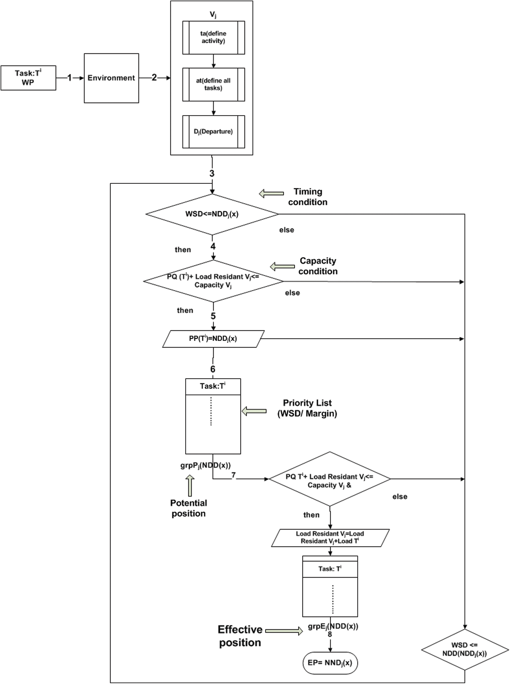
Figure 4: Determination of PP and EP for fixed departure with WSD/Margin

The tasks for which the capacity and timing condition are met, are grouped in grpP(NDDj(x)) and their potential position PPii=NDDj(x).

The tasks that do not meet the conditions are verified with subsequent departure list, such as, NDD(NDDj(x)).

In the case of effective position, the vehicle agent begins by verifying both conditions, i.e., timing and capacity of potential position. Here, the fundamental difference is that the tasks are aggregated until the vehicle is filled to the capacity. Vehicle vj finds the effective position EPii=NDDj(x) for all the tasks of grpE(NDDj(x))

The tasks that do not meet the conditions are verified with subsequent departure list, such as NDD(NDDj(x)), therefore:

5.3 Fixed Departure with Margin

Fixed departure with WSD is akin to Fixed Departure with Margin, that the vehicle agent begins by measuring both conditions but the priority list is now Prior(Margin)ai. The method is demonstrated in Fig. 4.

The tasks for which the capacity and timing are met, are grouped in grpP(NDDj(x))) and their potential position is represented by PPii=NDDj(x)

The tasks that do not meet the conditions are verified with subsequent departure list, such as NDD(NDDj(x)) such that:

The vehicle vj recommend the effective position EPii=NDDj(x) for all the tasks of grpE(NDDj(x)).

The tasks that do not meet the conditions are verified with subsequent departure list, such as NDD(NDDj(x))

5.4 Demand Responsive Departure with WSD

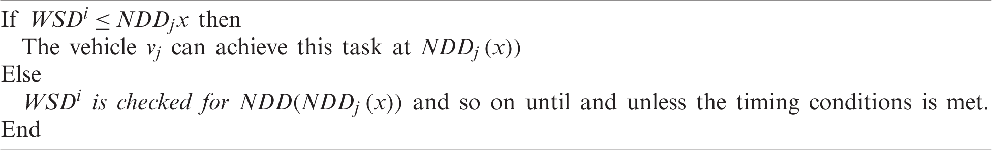
In the departure consideration for demand-responsive cases, the transport order pickup time is used as scheduled. So, in case a transport vehicle is unavailable at the activity origin place then the transport (whether with payload or vacant) will reach there after completing other task activities in its itinerary, Therefore, the vehicle's current location and payload condition determine the potential and effective position. The algorithm for finding a potential position is demonstrated via Fig. 4 and the algorithm for finding an effective position and related tasks is demonstrated through Fig. 5. The potential position finding method for vehicle vj uses Prior(WSD)ai, equation.

5.5 Demand Responsive Departure with Margin

Finding PP and EP for Demand responsive departure with Margin is similar to Demandresponsive departure with WSD method, using Prior(Margin)ai and the method for their determination are shown in Figs. 6 and 7.

6  Running Example

In order to test the functionality of the proposed algorithms for consolidation, a running example of the delivery of products in a supply chain is considered. This supply chain operates in the mountain areas of two countries of France and Spain called the Pyrenees. It consists of two product manufacturers, one is located in Spain (M-S) while the other is situated in France (M-F). This supply chain also consists of three logistics providers. First, TPL provider functions in the border area of France named TPL-F. Second, TPL provider functions in the border area of both France and Spain named TPL-FS. Third, TPL provider functions in the top north area of France named TPL-S. All of the logistics providers have their own fleet of vehicles and are specialized in food product delivery. Fig. 7 given below outlines the operating areas of all three logistics providers.

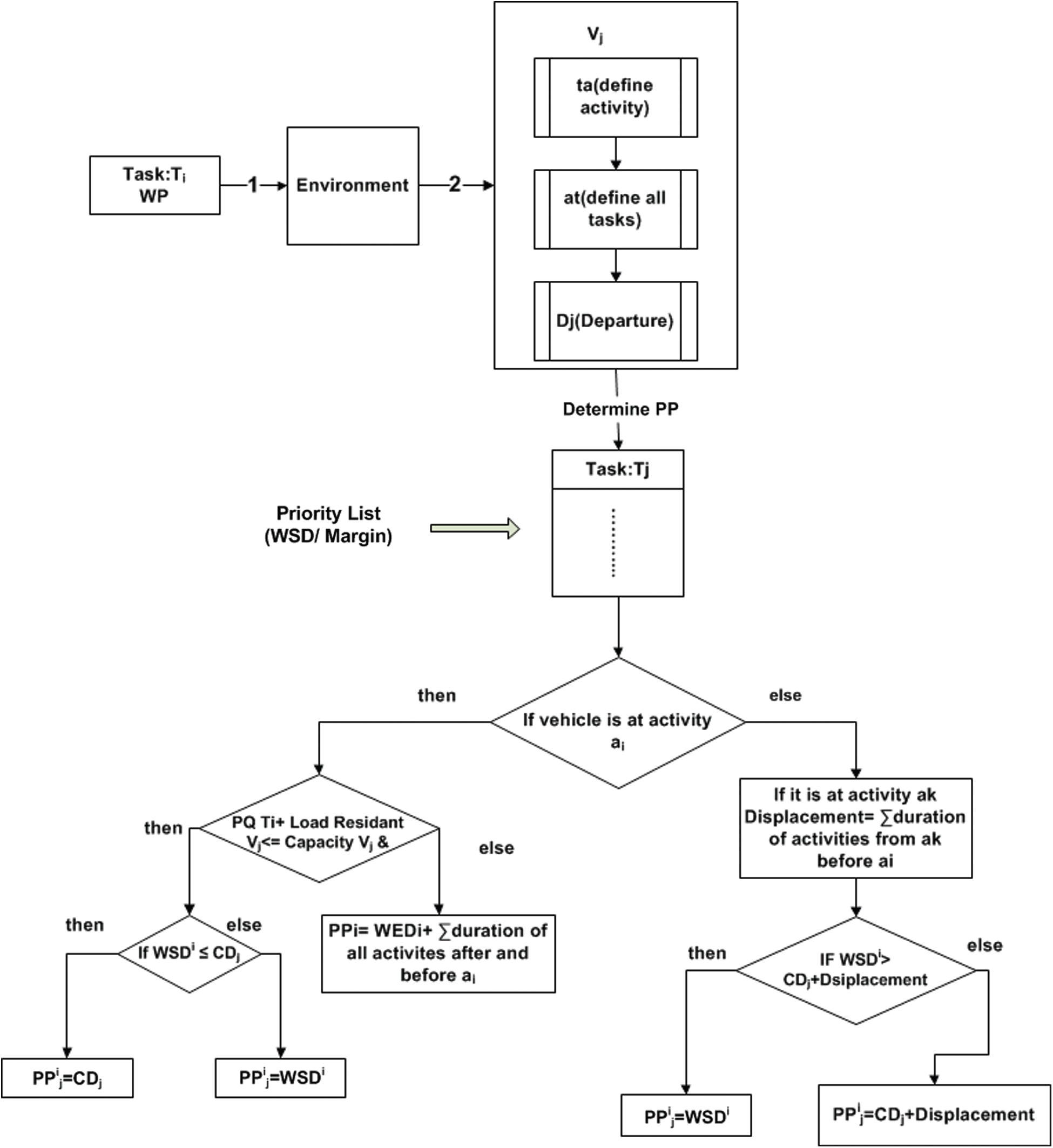
Figure 5: Determine PP for demand responsive departure with WSD/Margin

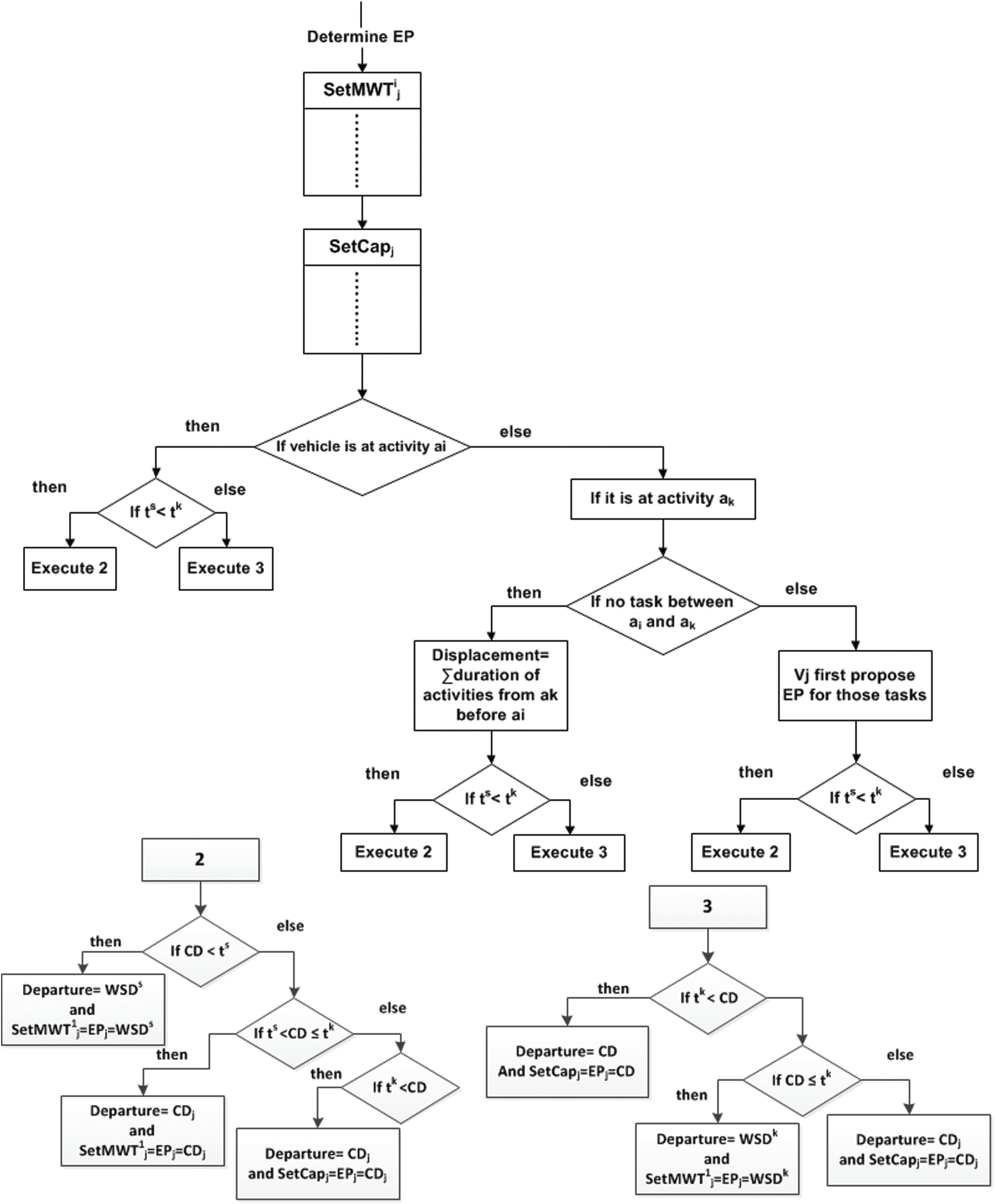
Figure 6: Determine EP for demand responsive departure with WSD/Margin

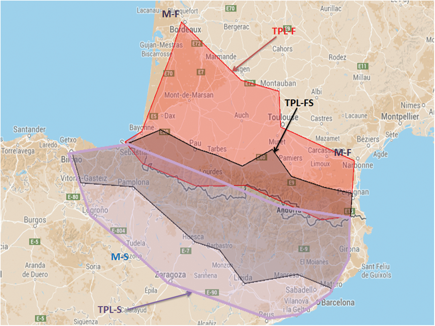
Figure 7: Supply chain operational area showing all the manufacturers and Logistics providers

The subsequent section is concerned with the presentation of the case study used to test the working rules proposed above.

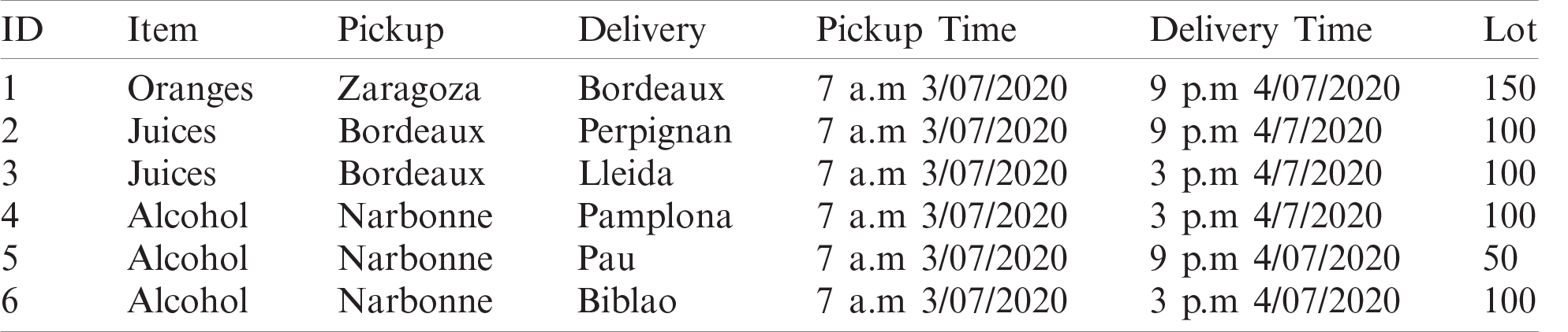
In this running example, the following delivery orders are considered from both manufacturers M-S and M-F in Tabs. 1 and 2 respectively.

Table 1: Delivery orders of manufacturers M-S

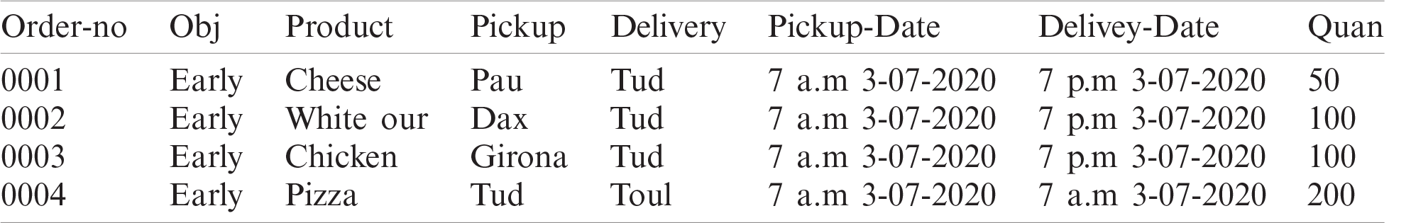
Table 2: Delivery orders of Manufacturer M-F

7  Result Analysis

In this section, an evaluation of scheduling results is presented. It is to be noted that the valuation presented here is based on the results obtained through all the rules except the last rule of DemandResponsiveDeparturewithMargin, which is not yet implemented. Fig. 8 given below shows the different parameters that are used for the performance analysis of scheduling rules. These parameters are

Cmax : Completion time

Tmax: Tardiness

Emax: Earliness

Avg(T): Average tardiness of the planning

Avg(E) : Average earliness of the planning

Avg(T) = ∑TOnTOimax(0,Cj--dj)∀i,…,n, where max(0,Cj--dj)≠0

Avg(E) = ∑TOnTOimax(0,dj--Cj)∀i,…,n, where max(0,dj--Cj)≠0

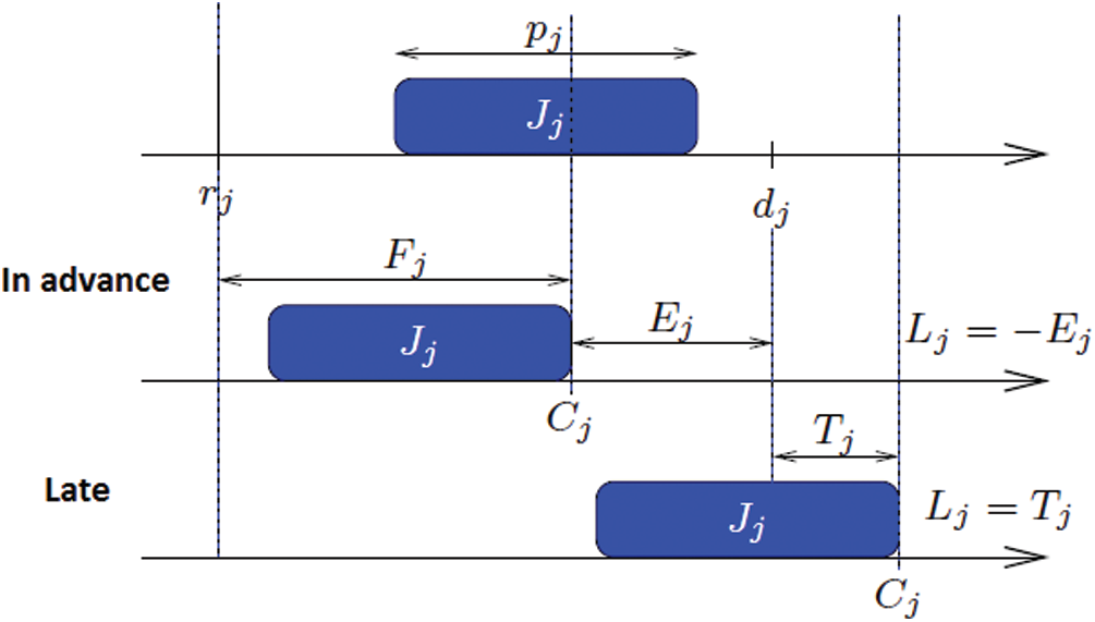
Figure 8: Standard criterion for evaluating planning

Cmax is the completion time of total planning when the order is finally delivered. Tab. 3 shows the final delivery time corresponding to each delivery order planned for the scheduling rule and Cmax value for each rule. Since the objective is the “Early” delivery, the DRD rule scheduled the early delivery of all orders before Fix-WSD and Fix-Margin rules. Moreover, Cmax Fix−WSD and Fix−Margin are quite near.

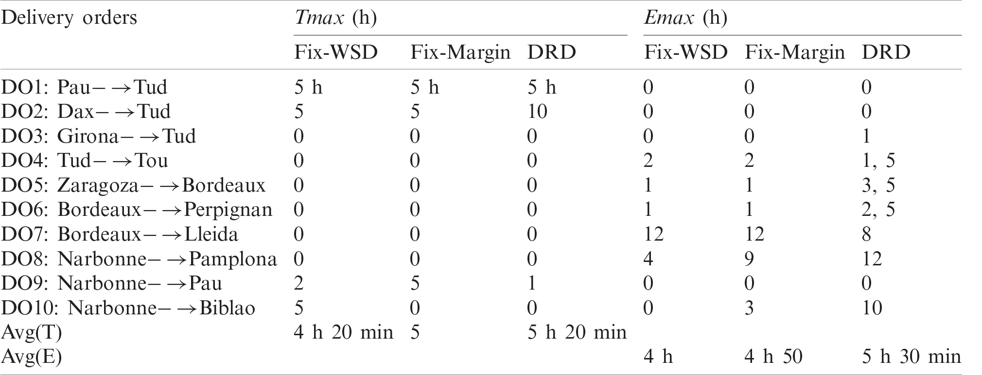
Tab. 4 details the parameters Tmax, Emax, for each delivery order for each rule and Avg(T) and Avg(E) for each rule.

Tmax is the time that a delivery order is delayed after its delivery date. It can be concluded from Tab. 4 that DO1, DO2, DO9, and DO10 are delivered after their due time, and DO2 is delivered in DRD is delivered with the duration almost double from Fix−WSD and Fix−Margin. On the whole, there is not much difference of delay in all the rules for Avg(T). A digit 0 in the column indicates the order is delivered on time or early.

Table 3: Delivery time for all delivery orders for each rule, and Cmax

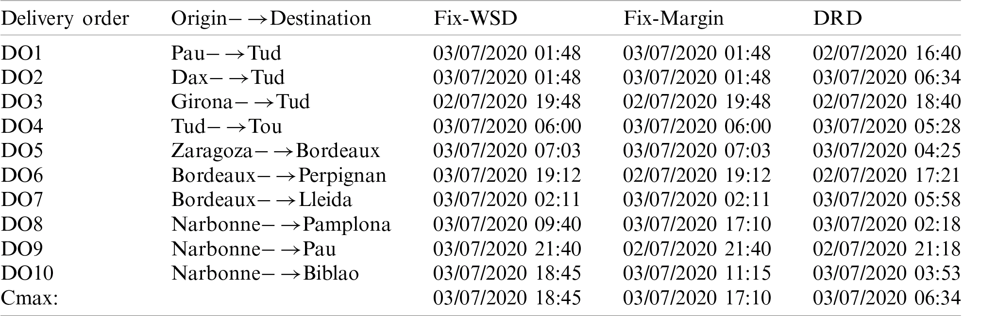
Table 4: Tmax, Emax, Avg(T) and Avg(E)

Emax is the time that a delivery order is delivered before the time of its delivery date. DO4, DO5, DO6, DO7, DO8 are scheduled for early delivery by all the rules. DO3 is delivered early in DRD rule. DO10 is planned early in the Fix-Margin rule but delivered with delay in DRD. Same as Avg(T), the value of Avg(E) is also very close in all the rules.

Taking into account, the delivery time set by the manufacturers for the delivery orders, delivery order DO3 is planned with on-time delivery. As the goal for all the delivery orders within the given example is the earliest delivery or on-time delivery. Hence Fix−WSD schedules 6 orders on time or before and Fix−Margin schedules 7 orders on time or before and DRD rule plans 7 orders on time or before. Hence, there is a 70% ratio of order delivery on time or before. It seems promising given the consolidation facilitation for minimizing the cost.

7.1 Occupancy Rate

Occupancy rate is to find out that how much time the vehicle is occupied throughout the delivery period from pick up until delivery. The occupancy rate can be calculated as the ratio of the vehicle during transportation and overall time through a certain time interval. Fig. 9. shows the graph of the occupancy rate of three rules for all the fleet of vehicles of TPL(s). It can be observed that the rate is 50%, which is almost the same for Fix−WSD and Fix−Margin. Though, for DRD, the rate is 90%, for vehicle FSV6, which is far better than the fixed departure rules. It is also noticed that the rate for vehicle SV7 is 0, making it unutilized in the whole scheduling process.

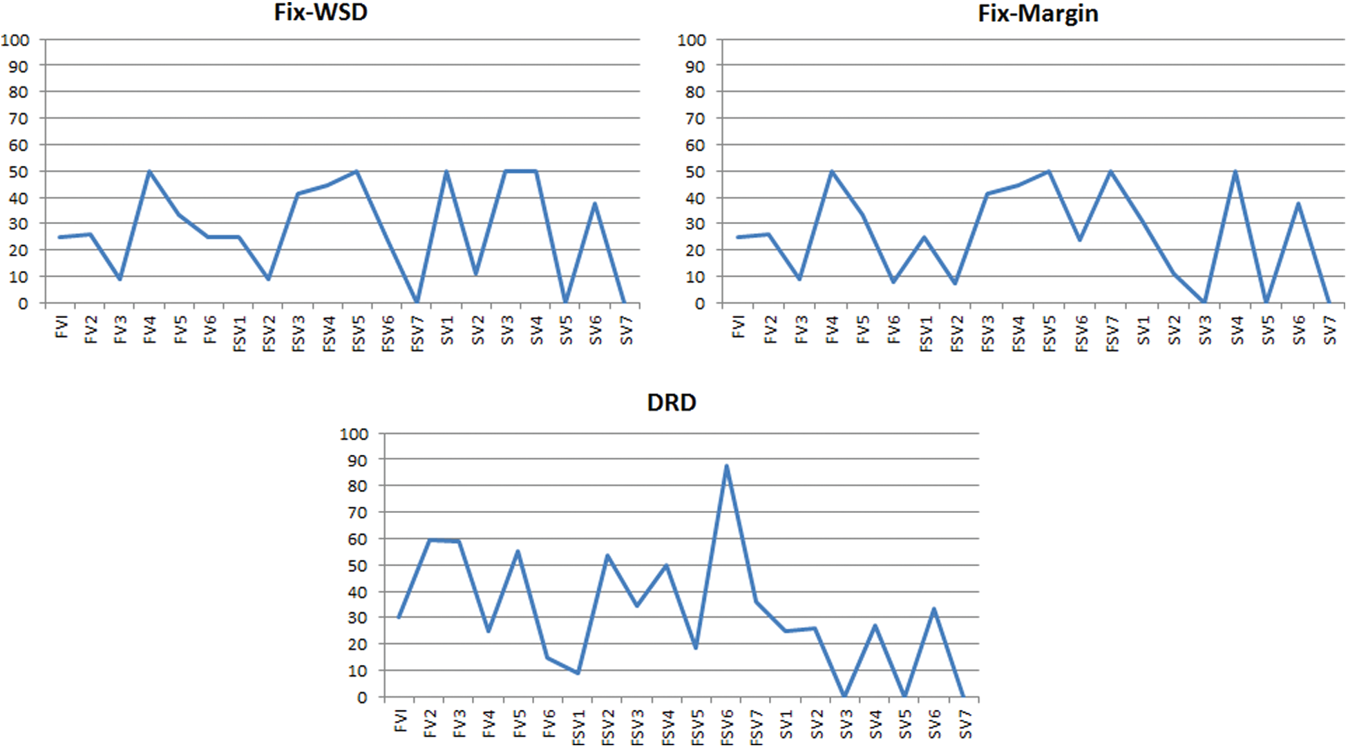
Figure 9: Occupancy rate of all the vehicles in all of the three rules

7.2 Consolidation

Fig. 10 shows that how many tasks are consolidated for each implemented rule. A total of 9 tasks are consolidated for Fix-WSD and Fix-Margin both making the rules of the same significance. Nonetheless, for DRD rule, a total of 15 tasks are consolidated, bringing the DRD in a better position in performance with the fixed departure rules.

7.3 Total Displacements Empty Trips excluding

In this section, we sum up the total number of displacements executed by all the vehicles for delivery. If two delivery orders are consolidated together for the delivery of the activity, it is even calculated as a single displacement. For the complete planning, there are 64 total tasks and for this criterion, we exclude the trips when the vehicle is traveling empty or without any order.

Fig. 11a explores the total number of displacements for Fix-WSD and Fix-Margin which are the same but for DRD it is slightly less. This difference can significantly increase with the rise in the total number of delivery orders.

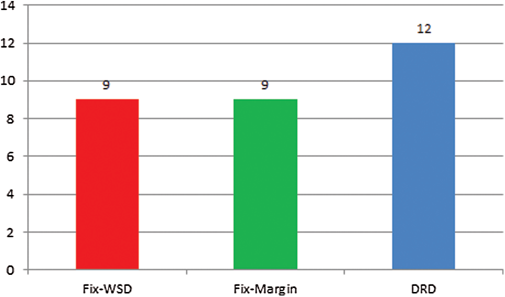
Figure 10: Total number of consolidated tasks in each rule

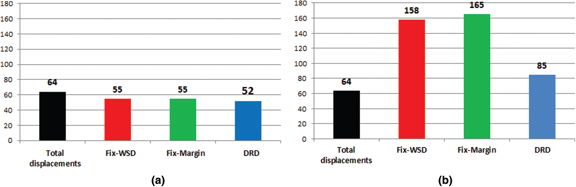
Figure 11: Total displacements (a) Empty trips excluding (b) Empty trips including

7.4 Total displacements Empty Trips Including

In this criterion, empty trips are included while calculating the total no of displacements. Condidering Fig. 11b, it can be noticed that total displacements for Fix-Margin are much higher, even more than Fix-WSD, but for DRD, the displacements are significantly less than other rules. These results more clearly illustrate the difference of supremacy of DRD rule over previous rules.

7.5 Total Distance Empty Trips Excluding

The value of this criterion is determined by adding the distance covered by all the vehicles excluding empty trips. Tab. 5 displays for each vehicle total distance covered within all three rules.

Table 5: Total distance covered by each vehicle in all the rules

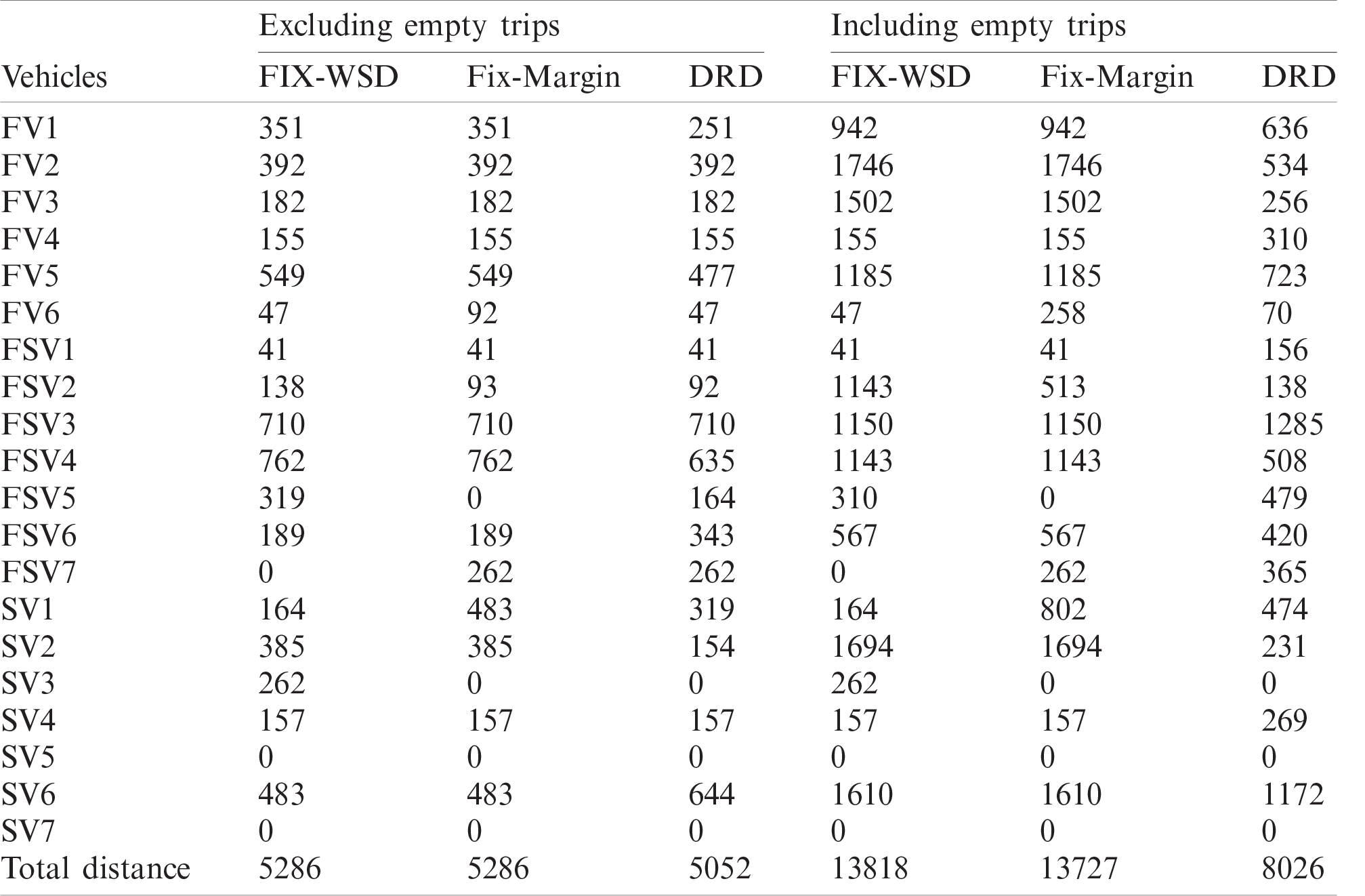
It can be seen that for total distance covered for trips excluding empty trips, there is no significant difference in any of the rules, however, including empty travels, DRD performs better than Fix-WSD and Fix-Margin.

It is observed from the overall analysis of the results achieved from the running example, Fix-Margin performs almost the same or slightly better as Fix-WSD especially in the case of a consolidation, which is the major concern of our work. On the other hand, DRD outclasses Fix-WSD and Fix-Margin in terms of performance in most of the criteria, more significantly in consolidation. Empty trips, occupancy rate, and the total distance are covered. Fixed departure considers the future arrival of delivery orders. It can be foreseen with the increasing number of delivery orders, Fix-WSD and Fix-Margin will also provide better results. Authors also assume that fixed route rules perform better under a high number of delivery orders demand.

8  Conclusions and Future Work

In this paper, a Hybrid (Time–Quantity Based) approach has been proposed to achieve the shipment consolidation of delivery orders varying with the number of products for delivery and Time of arrival. For this purpose, four algorithms have been proposed, out of which three have been implemented and tested on a pilot case study gathered from the industry. The results achieved cannot be deemed conclusive as only limited delivery orders have been considered. We conclude that the consolidation of delivery orders increases with each implemented rule. In the follow up, implementation of the fourth rule will be done on a priority basis, secondly, the vehicle's movement will be made flexible in order to reduce the order delay and empty travels, and finally, each result described here will be validated with a much bigger case study with varying scenarios.

Funding Statement: The authors would like to acknowledge the support of the Deputy for Research and Innovation, Ministry of Education, Kingdom of Saudi Arabia for this research through a grant (NU/IFC/INT/01/008) under the institutional Funding Committee at Najran University, Kingdom of Saudi Arabia.

Conflicts of Interest: The authors declare that they have no conflicts of interest to report regarding the present study.

References

 1.  S. K. Srivastava, “Green supply-chain management: A state-of-the-art literature review,” International Journal of Management Reviews, vol. 9, no. 1, pp. 53–80, 2007. [Google Scholar]

 2.  C. H. Glock, “A comparison of alternative delivery structures in a dual sourcing environment,” International Journal of Production Research, vol. 50, no. 11, pp. 3095–3114, 2012. [Google Scholar]

 3.  C. H. Glock, “Coordination of a production network with a single buyer and multiple vendors,” International Journal of Production Economics, vol. 135, no. 2, pp. 771–780, 2012. [Google Scholar]

 4.  T. Kim and S. K. Goyal, “A consolidated delivery policy of multiple suppliers for a single buyer,” International Journal of Procurement Management, vol. 2, no. 3, pp. 267–287, 2009. [Google Scholar]

 5.  D. O. Bausch, G. G. Brown and D. Ronen, “Consolidating and dispatching truck shipments of mobil heavy petroleum products,” Interfaces, vol. 25, no. 2, pp. 1–17, 1995. [Google Scholar]

 6.  G. Brown, J. Keegan, B. Vigus and K. Wood, “The kellogg company optimizes production, inventory, and distribution,” Interfaces, vol. 31, no. 6, pp. 1–15, 2001. [Google Scholar]

 7.  M. A. Ulku, “Dare to care: Shipment consolidation reduces not only costs, but also environmental damage,” International Journal of Production Economics, vol. 139, no. 2, pp. 438–446, 2012. [Google Scholar]

 8.  Y. P. Gupta and P. K. Bagchi, “Inbound freight consolidation under just-in-time procuremen,” Journal of Business Logistics, vol. 8, no. 2, pp. 74, 1987. [Google Scholar]

 9.  F. Mutlu and S. Cetinkaya, “An integrated model for stock replenishment and shipment scheduling under common carrier dispatch costs,” Transportation Research Part E: Logistics and Transportation Review, vol. 46, no. 6, pp. 844–854, 2010. [Google Scholar]

10. J. Marklund, “Inventory control in divergent supply chains with time-based dispatching and shipment consolidation,” Naval Research Logistics (NRL), vol. 58, no. 1, pp. 59–71, 2011. [Google Scholar]

11. F. Mutlu, S. I. L. Çetinkaya and J. H. Bookbinder, “An analytical model for computing the optimal time-and-quantity-based policy for consolidated shipments,” IIE Transactions, vol. 42, no. 5, pp. 367–377, 2010. [Google Scholar]

12. D. E. Blumenfeld, L. D. Burns, J. D. Diltz and C. F. Daganzo, “Analyzing trade-offs between transportation, inventory and production costs on freight networks,” Transportation Research Part B: Methodological, vol. 19, no. 5, pp. 361–380, 1985. [Google Scholar]

13. C. F. Daganzo, “The break-bulk role of terminals in many-to-many logistic networks,” Operations Research, vol. 35, no. 4, pp. 543–555, 1987. [Google Scholar]

14. C. F. Daganzo, “A comparison of in-vehicle and out-of-vehicle freight consolidation strategies,” Transportation Research Part B: Methodological, vol. 22, no. 3, pp. 173–180, 1988. [Google Scholar]

15. R. W. Hall, “Travel distance through transportation terminals on a rectangular grid,” Journal of the Operational Research Society, vol. 35, no. 12, pp. 1067– 1078, 1984. [Google Scholar]

16. R. W. Hall, “Determining vehicle dispatch frequency when shipping frequency differs among suppliers,” Transportation Research Part B: Methodological, vol. 19, no. 5, pp. 421–431, 1985. [Google Scholar]

17. A. Ülkü, “Dare to care: Shipment consolidation reduces not only costs, but also environmental damage,” International Journal of Production Economics, vol. 139, no. 2, pp. 438–446, 2012. [Google Scholar]

18. J. C. Tyan, F.-K. Wang and T. C. Du, “An evaluation of freight consolidation policies in global third party logistics,” Omega, vol. 31, pp. 55–62, 2003. [Google Scholar]

19. C. Nguyen, M. Dessouky and A. Toriello, “Consolidation strategies for the delivery of perishable products,” Transportation Research Part E: Logistics and Transportation Review, vol. 69, pp. 108–121, 2020. [Google Scholar]

20. J. Chen, M. Dong and L. Xu, “A perishable product shipment consolidation model considering freshness-keeping effort,” Transportation Research Part E: Logistics and Transportation Review, vol. 115, pp. 56–86, 2018. [Google Scholar]

21. D. Shejun, Y. Yuan, Y. Wang, H. Wang and C. Koll, “Collaborative multicenter logistics delivery network, optimization with resource sharing,” Plos One, vol. 15, no. 11, pp. 1–31, 2020. [Google Scholar]

22. J. D. Cortes and Y. Suzuki, “Vehicle routing with shipment consolidation,” International Journal of Production Economics, vol. 227, pp. 1–13, 2020. [Google Scholar]

23. N. L. Ma and K. W. Tan, “Reducing carbon emission through container shipment consolidation and optimization,” Journal of Traffic and Transportation Engineering, vol. 7, pp. 111–121, 2019. [Google Scholar]

24. L. Wei, S. Jasin and R. Kapuscinski, “Shipping consolidation with delivery deadline and expedited shipment options,” Ross School of Business Paper, paper no. 1375, pp. 1–45, 2017. [Online]. Available: SSRN: https://ssrn.com/abstract=2920899 or http://dx.doi.org/10.2139/ssrn.2920899. [Google Scholar]

25. A. S. Hanbazazah, L. Abril, M. Erkoc and N. Shaikh, “Freight consolidation with divisible shipments, delivery time windows, and piecewise transportation costs,” European Journal of Operational Research, vol. 276, pp. 87–201, 2019. [Google Scholar]

26. R. W. Hall, “Consolidation strategy: Inventory, vehicles and terminals,” Journal of Business Logistics, vol. 8, no. 2, pp. 57–73, 1987. [Google Scholar]

27. M. Estrada-Romeu and F. Robusté, “Stopover and hub-and-spoke shipment strategies in less-than-truckload carriers,” Transportation Research Part E: Logistics and Transportation Review, vol. 76, pp. 108–121, 2015. [Google Scholar]

28. D. J. Ford, “Inbound preight consolidation: A simulation model to evaluate consolidation rules,” in Massachusetts Institute of Technology, pp. 1–58, 2006. [Online]. Available: https://dspace.mit.edu/handle/ 1721.1/36145 (Accessed 02 March 2021). [Google Scholar]

29. J. Olsson and J. Woxenius, “Location of freight consolidation centres serving the city and its surroundings,” Procedia-Social and Behavioral Sciences, vol. 39, pp. 293–306, 2012. [Google Scholar]

30. A. Baykasoglu, V. Kapanoglu, R. Erol and C. Sahin, “A multi-agent framework for load consolidation in logistics,” Transport, vol. 26, no. 3, pp. 320–328, 2011. [Google Scholar]

31. M. Dror and B. C. Hartman, “Shipment consolidation: Who pays for it and how much?,” Management Science, vol. 53, no. 1, pp. 78–87, 2007. [Google Scholar]

32. T.-H. Chen and J.-M. Chen, “Optimizing supply chain collaboration based on joint replenishment and channel coordination,” Transportation Research Part E: Logistics and Transportation Review, vol. 41, pp. 261–285, 2005. [Google Scholar]

33. F. Mutlu and S. Çetinkaya, “An integrated model for stock replenishment and shipment scheduling under common carrier dispatch costs,” Transportation Research Part E: Logistics and Transportation Review, vol. 46, no. 6, pp. 844–854, 2010. [Google Scholar]

34. A. Ülkü, “Comparison of typical shipment consolidation programs: structural results,” Management Science and Engineering, vol. 3, no. 4, pp. 27–33, 2009. [Google Scholar]

35. J. H. Bookbinder and J. K. Higginson, “Probabilistic modeling of freight consolidation by private carriage,” Transportation Research Part E: Logistics and Transportation Review, vol. 38, no. 5, pp. 305–318, 2002. [Google Scholar]

36. S. Çetinkaya and J. H. Bookbinder, “Stochastic models for the dispatch of consolidated shipments,” Transportation Research Part B: Methodological, vol. 37, pp. 747–768, 2003. [Google Scholar]

37. D. Xu, M. A. Memon, B. Archimède and T. Coudert, “An environment friendly method to generate dynamic transportation routing in a distributed context,” in Int. Conf. on Industrial Engineering and Systems Management. Spain: Seville, pp. 702–707, 2015. [Google Scholar]

38. B. Archimède and T. Coudert, “Reactive scheduling using a multi-agent model: The SCEP framework,” Engineering Applications of Artificial Intelligence, vol. 14, no. 5, pp. 667–683, 2001. [Google Scholar]

39. T. Coudert, “Apport des systèmes multi-agents pour la négociation en ordonnancement: Application aux fonctions production et maintenance,” Doctoral Dissertation, Toulouse, INPT, 2000. [Online]. Available: https://www.theses.fr/2000INPT014G (Accessed 02 March 2021). [Google Scholar]

This work is licensed under a Creative Commons Attribution 4.0 International License, which permits unrestricted use, distribution, and reproduction in any medium, provided the original work is properly cited.