Stress Distribution in Composites with Co-Phase Periodically Curved Two Neighboring Hollow Fibers

Kosker, Resat; Gulten, Ismail

doi:10.32604/cmc.2021.017857

[BACK]

Computers, Materials & Continua DOI:10.32604/cmc.2021.017857
Article

Stress Distribution in Composites with Co-Phase Periodically Curved Two Neighboring Hollow Fibers

Resat Kosker1,*and Ismail Gulten2

1Department of Mathematical Engineering, Faculty of Chemistry and Metallurgy, Yildiz Technical University, Davutpasa Campus, Esenler, 34220, Istanbul, Turkey
2Department of Mathematical Engineering, Graduate School of Natural and Applied Sciences, Yildiz Technical University, Davutpasa Campus, Esenler, 34220, Istanbul, Turkey
*Corresponding Author: Resat Kosker. Email: kosker@yildiz.edu.tr
Received: 14 February 2021; Accepted: 04 April 2021

Abstract: In this paper, stress distribution is examined in the case where infinite length co-phase periodically curved two neighboring hollow fibers are contained by an infinite elastic body. The midline of the fibers is assumed to be in the same plane. Using the three-dimensional geometric linear exact equations of the elasticity theory, research is carried out by use of the piecewise homogeneous body model. Moreover, the body is assumed to be loaded at infinity by uniformly distributed normal forces along the hollow fibers. On the inter-medium between the hollow fibers and matrix surfaces, complete cohesion conditions are satisfied. The boundary form perturbation method is used to solve the boundary value problem. In this investigation, numerical results are obtained by considering the zeroth and first approximations to calculate the self-equilibrium shear stresses and normal stress at the contact surfaces between the hollow fibers and matrix. Numerous numerical results have been obtained and interpreted about the effects of the interactions between the hollow fibers on this distribution.

Keywords: Hollow fibers; stress distribution; fibrous composite; periodic curvature

1 Introduction

Composite materials have increased in importance as they have superior properties than the materials they are made of. Today, composites have numerous application areas such as energy, sports, military, automotive, marine, aerospace, civil engineering, biomedical and even the music industry [1]. Unidirectional fibrous composites have an important place among composite materials. It is very important to create a mathematical model about the elastic behavior of these materials so that they are used effectively in practice when exposed to various external influences, and to examine them theoretically. These investigations will determine the rheological, mechanical, thermal, electrical and morphological properties of the materials. For example, it has been found that fibrous composites with well-dispersed reinforcing fibers have higher electrical and thermal conductivity [1–3].

As noted in [4–6], one of the main factors that determines the strength of unidirectional fibrous composite is the fibers’ curvature. Curvature can occur as a result of design or as a result of a technological process and is called periodic or local. Practical applications of these composite materials require determination of the stress-strain state considering the curl of the fibers. Self-balanced stresses arise due to the curvature of the fibers, and these stresses can cause the fibers to separate from the matrix under uniaxial tension or stress along the fibers [5,7,8]. This separation leads to the formation of macro cracks, whose accumulation can significantly alter the strength and stiffness properties of the composites [9]. In addition, the initial minor curling of reinforcing fibers is taken as a model for investigating various stability loss or fracture problems of unidirectional composites [10]. Therefore, creating the mechanics of composite materials containing curved structures is important both in terms of fundamental advances in the mechanics of rigid deformable bodies and in modern engineering that uses special composite components. In [11], to achieve this aim, using the three-dimensional exact equations of the elasticity theory together with the piecewise homogenous body model, a method was developed for investigating the stress-strain state produced in unidirectional fibrous composite materials. Fiber curving was considered periodic in that study. Reviews of the numerical results obtained by using this method are given in [5].

The method discussed in [11] is proposed for the case where the concentration of fibers is so small that the interactions between them are negligible. In [12], the method is developed to be used in the problem of two neighboring periodically inclined fibers, and numerical results are given taking into account the interaction between the fibers. In [13], this method is extended to the nonlinear geometric state, and from here, the numerical results obtained for stresses in a composite material containing one and two neighboring periodically inclined fibers are presented. Studies on the loss of stability problems corresponding to these conditions are reviewed in [14]. In [15–18], this approach is developed for a periodically located row of fibers embedded in an infinite matrix and the obtained numerical results are presented. In [19], the stability loss of the related problem is studied. In addition, some similar studies in the local curvature case are presented in publications [20–23].

However, in all the investigations given above, it is assumed that the fibers embedded in the matrix are traditional materials. In [24], the reinforcing element is taken as a double-walled carbon nanotube (DWCNT), and the loss of internal stability in composite materials containing a straight infinitely long DWCNT is examined. In [25], the stress distribution is studied in an infinite body containing an infinite length periodically curved hollow fiber with low concentration. In this study, to calculate the effect of the interactions between the hollow fibers on the stresses, the same situation is developed for the two neighboring hollow fiber cases. The problem is the stress distribution in the infinite body containing infinite length, periodically curved two neighboring hollow fibers. The investigations are made by using the three-dimensional geometric linear exact equations of the elasticity theory with the piecewise homogeneous body model. In addition, it is assumed that uniformly distributed normal forces are acting on the body at infinity along the hollow fibers.

2 Mathematical Formulation of the Problem

Infinite length, periodically curved two neighboring hollow fibers embedded in an infinite elastic body are taken into account. We assume that the perpendicular sections of the hollow fibers are circles with radius R and thickness H and this does not change throughout the hollow fibers. We also note that the midline of the hollow fibers is in the same plane and has co-phase initial periodic tilting with respect to each other. In the aforementioned model, it is thought that there are normal forces with intensity p that are evenly distributed in the longitudinal direction of the hollow fibers.

Let us select Omxm1xm2xm3 cartesian and Omrmθmzm cylindrical coordinate sets for the centerline of each hollow fiber as the Lagrange coordinates (Fig. 1). Here, m=1,2, shows the first and second hollow fibers, respectively. As can be seen from Fig. 1, between these coordinates the following relations are satisfied:

x12=x22,x13=x23,r1eiθ1=R12+r2eiθ2,z1=z2=z(1)

Assuming that the midlines of the hollow fibers are in the x12=x22=0 plane, the equations of these lines are written as follows:

x11=Lsin(2πℓx13),x21=Lsin(2πℓx23)(2)

Here, L is the bending amplitude of the hollow fibers and ℓ is the period of bending. Assuming that L is much smaller than ℓ, let us define the ε=L/ℓ parameter (0<ε<<1). The degree of initial defect of the hollow fibers is characterized by this parameter.

In the following, we will show the values belonging to the first and second hollow fibers with the superscript (21) and (22), respectively and the values belonging to the matrix (infinite elastic medium) with the superscript (1).

images

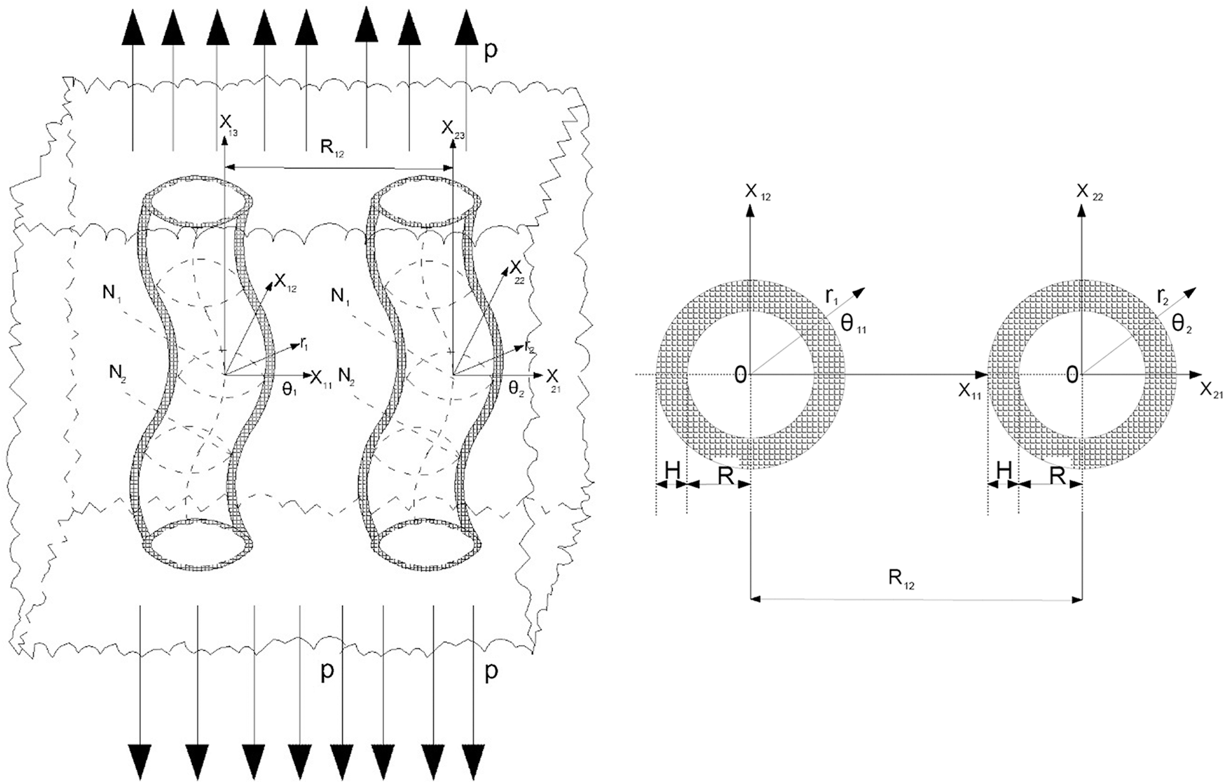
Figure 1: Geometry and coordinate systems of the considered material structures

Let us write the following governing field equations to be satisfied in each hollow fiber and infinite elastic medium:

∇i[σ(k_)in(gnj+∇nu(k_)j)]=0,2εjm(k)=∇jum(k)+∇muj(k)+∇ju(k_)n∇mun(k_),

σ(in)(k)=(λ(k_)e(k_))δin+2(μ(k_)ε(in)(k_)),e(k)=εrr(k)+εθθ(k)+εzz(k)(3)

Let us denote the inner surface of the hollow fibers with S0k (k=1,2) and the outer surface (the contact surface with the matrix) with Sk (k=1,2). We write the contact conditions below, assuming that the inner radii of the hollow fibers remain constant and that there are ideal contact conditions between the hollow fibers and the matrix.

σ(2k_)in(gnj+∇nu(2k_)j)|S0k_nk_j=0,σ(2k_)in(gnj+∇nu(2k_)j)|Sk_nk_j=σ(1)in(gnj+∇nu(1)j)|Sk_nk_j,

uj(2k_)|Sk_=uj(1)|Sk_,k=1,2(4)

In the case discussed, the following conditions are also provided:

σzz(1)⟶z→∞p,σ(ij)(1)⟶rk→∞0(ij)≠(zz)(5)

Tensor notation is used in the formulae given above. We should state that the sum cannot be made according to the underlined indices.

Thus, the formulation of the addressed problem is completed. The problem is reduced to the solution of Eq. (3) within the framework of (4) contact and (5) boundary conditions.

3 Solution of the Problem

We can write the equations of the surfaces Sk and S0k from the cross-sectional form condition of the hollow fibers.

rk= (1+ε2(δk_′(t3))2sin2θk_)−1{(εδk_(t3)+ε3δk_(t3)(δk_′(t3))2)sinθk_+[(R+H)2−ε2(δk_(t3))2−ε4(δk_′(t3))2(δk_(t3))2(1+ε2(δk_′(t3))2)sin2θk_]12}

zk=t3−εδk_′(t3)rk_(t3)sinθk_+ε2δk_(t3)δk_′(t3),δk′(t3)=dδk(t3)dt3,δk(t3)=ℓsin(2πℓt3)(6)

Here, t3∈(−∞,+∞) is a parameter. Using Eq. (6) and doing some known operations, we obtain the following expressions for the components of the unit external normals of Sk surfaces:

nkr=rk(θk_,t3)∂zk_(θk_,t3)∂t3[Ak_(θk_,t3)]−1nkθ=[∂zk_(θk_,t3)∂θk_∂rk_(θk_,t3)∂t3−∂rk_(θk_,t3)∂θk_∂zk_(θk_,t3)∂t3][Ak_(θk_,t3)]−1

nkz=−rk_(θk_,t3)∂rk_(θk_,t3)∂t3[Ak_(θk_,t3)]−1(7)

Ak_(θk_,t3)=[(rk_(θk_,t3)∂zk_(θk_,t3)∂t3)2+(∂zk_(θk_,t3)∂θk_∂rk_(θk_,t3)∂t3−∂zk_(θk_,t3)∂t3∂rk_(θk_,t3)∂θk_)2+(rk_(θk_,t3)∂rk_(θk_,t3)∂t3)2]12(8)

The boundary-form perturbation method given in [5] will be used to examine this problem. According to this method, all the expressions are searched in series form in terms of the small parameter defined above.

{σ(ij)(m);ε(ij)(m);u(i)(m)}=∑q=0∞εq{σ(ij)(m),q;ε(ij)(m),q;u(i)(m),q}(9)

Expressions (6) and (7) are also written serially according to ε:

rk=R+∑q=1∞εqak_q(θk_,t3),zk=t3+∑q=1∞εqbk_q(θk_,t3),nkr=1+∑q=1∞εqck_q(θk_,t3),nkθ=∑q=1∞εqdk_q(θk_,t3),

nkz=∑q=1∞εqgk_q(θk_,t3).(10)

The aq_k(θq_,t3),bk_q(θk_,t3),ck_q(θk_,t3),dk_q(θk_,t3), and gk_q(θk_,t3) in these expressions, which are the coefficients of εk, can be easily obtained from (6)–(8). From (3), the governing field equations provided separately for each approach in (9) are obtained. If we use (10), we open each approach in (9) to a series around (rk=R+H, θk, t3) and (rk=R, θk, t3). If we substitute these last statements in (4) and use the expressions of nqr, nqθ, nqz in (10), then as a result of some long but known operations, the contact conditions provided in rk=R+H and rk=R, for each approach in (9) are obtained. In this case, the k-th contact condition includes the sizes of all the previous k-1 approaches.

We will deal with the case where the nonlinear terms in the equations related to the zeroth approximation can be omitted, and since ∇nu(k)j,0<<1, δnj in the first and other approaches can replace (gnj+∇nu(k)j,0). In addition, we will assume that the σ(ij)(k),0 (ij)≠zz stresses in the zeroth approximation can be neglected as well as the σzz(k),0 stresses [15]. According to this assumption, the governing field equations and contact conditions of the zeroth approach are obtained as follows:

∇iσ(k)ij,0=0,2εij(k),0=∇jui(k),0+∇iuj(k),0,

σ(in)(k),0=(λ(k_)e(k_),0)δin+2(μ(k_)ε(in)(k_),0),e(k),0=εrr(k),0+εθθ(k),0+εzz(k),0(11)

σ(ij)(2k),0|rk=R=0,σ(ij)(2k),0|rk=R+H=σ(ij)(1),0|rk=R+H,

u(i)(2k),0|rk=R+H=u(i)(1),0|rk=R+H;(ij)=rr,rθ,rz,(i)=r,θ,z;k=1,2(12)

Thus, the zeroth approach is reduced to the solution of Eq. (11) within the framework of contact conditions (12).

For the first approach, we can write the governing field equations as follows:

∇i[σ(k)ij,1+σ(k)in,0∇nu(k)j,1]=0(13)

2εij(k),1=∇jui(k),1+∇iuj(k),1(14)

σ(in)(k),1=(λ(k_)e(k_),1)δin+2(μ(k_)ε(in)(k_),1),e(k),1=εrr(k),1+εθθ(k),1+εzz(k),1(15)

For this approach, we obtain the contact conditions as follows:

[σ(i)r]2k,1+f1k_[∂σ(i)r∂r]2k_,0+ϕ1k_[∂σ(i)r∂z]2k_,0+γrk_[σ(i)r]2k_,0+γθk_[σ(i)θ]2k_,0+γzk_[σ(i)z]2k_,0=0[σ(i)r]1,12k,1+f1k_[∂σ(i)r∂r]1,02k_,0+ϕ1k_[∂σ(i)r∂z]1,02k_,0+γrk_[σ(i)r]1,02k_,0+γθk_[σ(i)θ]1,02k_,0+γzk_[σ(i)z]1,02k_,0=0

[u(i)]1,12k,1+f1k_[∂u(i)∂r]1,02k_,0+ϕ1k_[∂u(i)∂z]1,02k_,0=0(16)

where

[ϕ]2k,s=ϕ(2k),s,[ϕ]1,s2k,s=ϕ(2k),s−ϕ(1),s;f1k=δk_(t3)cosθk_;ϕ1k=−Rδk_′(t3)cosθk_,

γrk=(δk_(t3)R−δk_″(t3)R)cosθk_;γθk=−δk_(t3)Rsinθk_;γzk=−δk_′(t3)cosθk_;k=1,2(17)

In this section, we will obtain the solutions of the boundary-value problems of the zeroth and first approaches formulated above. For simplicity, we will assume that both fiber materials are the same and that Poisson's ratio of ν(21)=ν(22)=ν(2) (ν(2k) k-th fiber to Poisson's ratio) is equal to Poisson's ratio of the matrix material which we will show as ν(1).

In this case, we get the following solution for the zeroth approach:

σzz(1),0=p;σzz(21),0=σzz(22),0=E(2)E(1)p;εzz(21),0=εzz(22),0=εzz(1),0=pE(1);z=z1=z2

uz(21),0=uz(22),0=uz(1),0=εzz(1),0z;σ(ij)(2q),0=σ(ij)(1),0=0;(ij)=rr,θθ,rθ,θz,rz(18)

E(1) and E(2) in (18) are the elasticity moduli of the matrix and fiber materials, respectively.

Let us now consider the solution of the problem (13)–(17) belonging to the first approach. Considering the above assumptions and the solution of the zeroth approach (18), the Eq. (13) are obtained as follows:

∂σrr(k_),1∂rk_+1rk_∂σrθ(k_),1∂θk_+∂σrz(k_),1∂zk_+1rk_(σrr(k_),1−σθθ(k_),1)=0,∂σrθ(k_),1∂rk_+1rk_∂σθθ(k_),1∂θk_+∂σθz(k_),1∂zk_+2rk_σrθ(k_),1=0,

∂σrz(k_),1∂rk_+1rk_∂σθz(k_),1∂θk_+∂σzz(k_),1∂zk_+1rk_σrz(k_),1=0(19)

These equations coincide with the linearized three-dimensional elasticity equations. Similarly, Eq. (14) become:

εrr(k),1=∂ur(k_),1∂rk_,εrθ(k),1=12(1rk_∂ur(k_),1∂θk_+∂uθ(k_),1∂rk_−uθ(k_),1rk_),εrz(k),1=12(∂uz(k_),1∂rk_+∂ur(k_),1∂zk_)

εθθ(k),1=1rk_∂uθ(k_),1∂θk_+ur(k_),1rk_,εθz(k),1=12(∂uθ(k_),1∂zk_+1rk_∂uz(k_),1∂θk_)εzz(k),1=∂uz(k_),1∂zk_(20)

Considering the solution obtained in the zeroth approach, the contact conditions of the first approach (16) are obtained as follows:

[σrr]2k,1=0,[σrθ]2k,1=0,[σrz]2k,1=δk_′(t3)σzz(2),0cosθk_,[σrr]1,12k,1=0,[σrθ]1,12k,1=0,[σrz]1,12k,1=δk_′(t3)(σzz(1),0−σzz(2),0)cosθk_,

[ur]1,12k,1=0,[uθ]1,12k,1=0,[uz]1,12k,1=0(21)

For the solution of Eq. (21), let us use the following representation given in [5], taking into account (19):

ur(k),1=1rk_∂∂θk_ψ(k_)−∂2∂rk_∂zχ(k_),uθ(k),1=−∂∂rk_ψ(k_)−1rk_∂2∂θk_∂zχ(k_),Δ1(k)=∂2∂rk2+1rk_∂∂rk_+1rk_2∂2∂θk_2,

uz(k),1=(λ(k_)+μ(k_))−1((λ(k_)+2μ(k_))Δ1(k_)+(μ(k_)+σzz(k),0)∂2∂z2)χ(k_);(22)

The ψ(k) and χ(k) functions here provide the following equations:

(Δ1(k_)+(ξ1(k_))2∂2∂z2)ψ(k_)=0,

(Δ1(k_)+(ξ2(k_))2∂2∂z2)(Δ1(k_)+(ξ3(k_))2∂2∂z2)χ(k_)=0(23)

ξi(k) (k=21,22,1;i=1,2,3) in (23) are fixed as follows:

ξ1(k)=μ(k_)+σzz(k_),0μ(k_),ξ2(k)=μ(k_)+σzz(k_),0μ(k_),ξ3(k)=λ(k_)+2μ(k_)+σzz(k_),0λ(k_)+2μ(k_)(24)

Thus, the solution of Eq. (23) is obtained by considering the expressions on the right side of Eq. (21) as follows:

ψ(1),1=αsinαz∑k=12∑n=−∞∞Cn(1)kKn(ξ1(1)α rk) exp (inθk)

χ(1),1=cosαz∑k=12∑n=−∞∞[An(1)kKn(ξ2(1)αrk)+Bn(1)kKn(ξ3(1)αrk)]exp (inθk)(25)

ψ(2k),1=αsinαz∑n=−∞∞{Cn(2k_)In(ξ1(2k_)αrk_)+Dn(2k_)Kn(ξ1(2k_)αrk_)}exp(inθk_)

χ(2k),1=cosαz∑n=−∞∞{An(2k_)In(ξ2(2k_)αrk_)+Bn(2k_)In(ξ3(2k_)αrk_)+En(2k_)Kn(ξ2(2k_)αrk_)+Fn(2k_)Kn(ξ3(2k_)αrk_)}exp(inθk_)(26)

In (25) and (26), α=2π/ℓ and In(x),Kn(x) are the Bessel functions with imaginary arguments and Macdonald functions, respectively. An(1)k,Bn(1)k,Cn(1)k, An(2k),Bn(2k),Cn(2k),Dn(2k),En(2k), and Fn(2k) unknowns are complex constants and provide the following relationships:

An(1)k=A−n(1)k¯,Bn(1)k=B−n(1)k¯,Cn(1)k=C−n(1)k¯,Im(A0(1)k)=Im(B0(1)k)=Im(C0(1)k)=0An(2k)=A−n(2k)¯,Bn(2k)=B−n(2k)¯,Cn(2k)=C−n(2k)¯,Im(A0(2k))=Im(B0(2k))=Im(C0(2k))=0

Dn(2k)=D−n(2k)¯,En(2k)=E−n(2k)¯,Fn(2k)=F−n(2k)¯,Im(D0(2k))=Im(E0(2k))=Im(F0(2k))=0(27)

In order to write the (r2,θ2) coordinates in (r1,θ1) coordinates or, on the contrary, (r1,θ1) in (r2,θ2) coordinates, we will make use of the summation theorem [26] and the relations between cylindrical coordinate sets.

rm_exp iθm_=Rm_n_exp iϕm_n_+rn_exp iθn_Kν(crn_)exp iνθn_=∑k=−∞∞(−1)νIk(crm_)Kν−k(cRm_n_)exp[i(ν−k)ϕm_n_]exp ikθm_

mn=12;21;m;n=1,2;rm<Rmn;R12=R21;ϕ12=0;ϕ21=π.(28)

Thus, an infinite dimensional system of algebraic equations is obtained from (21) in terms of unknown constants (27) by using (22)–(26). If this system is solved using the convergence criterion and the unknowns are determined, then the desired stress values are determined. Let us show that the convergence criterion is satisfied in order for this system to be replaced by a finite one. Let us introduce the following notations:

Cn(2k)In(ξ1(2)κ1)=yn1(2)k+izn1(2)k,An(2k)In(ξ2(2)κ1)=zn2(2)k+iyn2(2)k,Bn(2k)In(ξ3(2)κ1)=zn3(2)k+iyn3(2)kDn(2k)Kn(ξ1(2)κ1)=yn1(2)k+izn1(2)k,En(2k)Kn(ξ2(2)κ1)=zn2(2)k+iyn2(2)k,Fn(2k)Kn(ξ3(2)κ1)=zn3(2)k+iyn3(2)kCn(1)kKn(ξ1(1)κ2)=yn1(1)k+izn1(1)k,An(1)kKn(ξ2(1)κ2)=zn2(1)k+iyn2(1)k,Bn(1)kKn(ξ3(1)κ2)=zn3(1)k+iyn3(1)kCn(2k)In(ξ1(2)κ2)=yn1(3)k+izn1(3)k,An(2k)In(ξ2(2)κ2)=zn2(3)k+iyn2(3)k,Bn(2k)In(ξ3(2)κ2)=zn3(3)k+iyn3(3)kDn(2k)Kn(ξ1(2)κ2)=yn1(3)k+izn1(3)k,En(2k)Kn(ξ2(2)κ2)=zn2(3)k+iyn2(3)k,Fn(2k)Kn(ξ3(2)κ2)=zn3(3)k+iyn3(3)kZn(k)q=[zn1(k)qzn2(k)qzn3(k)q],Yn(k)q=[yn1(k)qyn2(k)qyn3(k)q],Tnm(1)q=[trs(1)q(n,m)],Tn(2)q=[trs(2)q(n)],Wnv(1)q=[wrs(1)q(n,v)],

Wn(2)q=[wrs(2)q(n)],q=1,2;k=1,2,3;r;s=1,2,3,κ1=2πRℓ,κ2=2π(R+H)ℓ(29)

The system of infinite algebraic equations in terms of defined notations is written as:

Zn(1)1+∑m=0∞Tnm(1)2Zm(1)2+Tn_(2)1Zn_(2)1=0,Zn(1)2+∑m=0∞Tnm(1)1Zm(1)1+Tn_(2)2Zn_(2)2=0(30)

Yn(1)1+∑m=0∞Wnm(1)2Ym(1)2+Wn_(2)1Yn_(2)1=2πδn3σzz(21),0

Yn(1)2+∑m=0∞Wnm(1)1Ym(1)1+Wn_(2)2Yn_(2)2=2πδn3σzz(22),0(31)

Zn(1)1+∑m=0∞Tnm(1)2Zm(1)2+Tn_(2)1Zn_(3)1=0,Zn(1)2+∑m=0∞Tnm(1)1Zm(1)1+Tn_(2)2Zn_(3)2=0(32)

Yn(1)1+∑m=0∞Wnm(1)2Ym(1)2+Wn_(2)1Yn_(3)1=2πδn3(σzz(1),0−σzz(21),0)

Yn(1)2+∑m=0∞Wnm(1)1Ym(1)1+Wn_(2)2Yn_(3)2=2πδn3(σzz(1),0−σzz(22), 0),n=0,1,2,…,∞; δnm={1m=n0m≠n(33)

It is obtained from (31) and (33) that Zn(k)q=0, k=1,2 and q=1,2. Also, from mechanical considerations and Eqs. (31) and (33), it is seen that Yn(k)1=Yn(k)2. Thus, from (31) and (33) we get the following:

Yn(1)1+∑m=0∞Wnm(1)2Ym(1)2+Wn_(2)1Yn_(2)1=2πδn3σzz(2),0

Yn(1)1+∑m=0∞Wnm(1)2Ym(1)2+Wn_(2)1Yn_(3)1=2πδn3(σzz(1),0−σzz(2),0)(34)

The infinite system of algebraic Eq. (34) must be approximated by the finite one to obtain numerical results. To make this displacement possible, the determinant of the algebraic infinite system of equations must be of normal type [27]. This is achieved if we show that the following series is convergent:

M=∑n=0∞∑m=0∞|Wnm(1)2|(35)

The functions In(x) and Kn(x) are satisfied in the following asymptotic estimates:

In(x)<c11n!(|x|2)n,Kn(x)≈c2(n−1)!(2|x|)n,n→∞,c1,c2 are constants.(36)

Since the hollow fibers do not touch each other, the following inequalities are achieved:

(R+H)/(R12−2L)>(R+H)/R12,R12/(R+H)>2(37)

From (36)–(37), and analyzing Wnm(1)2, we show the convergence of the series (35) as follows:

M<c3∑n=0∞nc4(R12R+H−1)−n,c3,c4 const.(38)

Similar proof is made in [11,12]. Thus, the infinite algebraic system can be replaced by a finite one. The number of equations the finite system will consist of, will be decided by the convergence of the numerical results.

4 Numerical Results

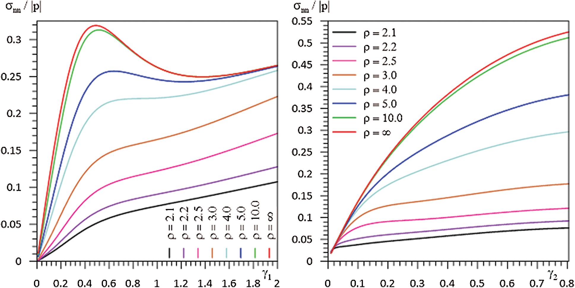
In this study, the numerical results have been obtained using the zeroth and first approximations. Next approaches can only contribute quantitatively to the results. In addition, Poisson ratios are taken as ν(1)=ν(2)=0.3, and the dimensionless parameter ρ=R12/(R+H), which shows the contribution of the interaction of hollow fibers to the stress values, is defined. Furthermore, by examining the contribution of the parameters E=E(2)/E(1), γ1=2π(R+H)/ℓ=α(R+H) and γ2=H/(R+H) to the stress distribution, the ratio of elasticity modulus and the effect of the thickness and radius of the hollow fibers will be calculated. While calculating the stresses, since they have maximum values, θ=0,αt3=π/2 for σnn, θ=0,αt3=0 for σne and θ=0,αt3=0 for σnτ are used.

images

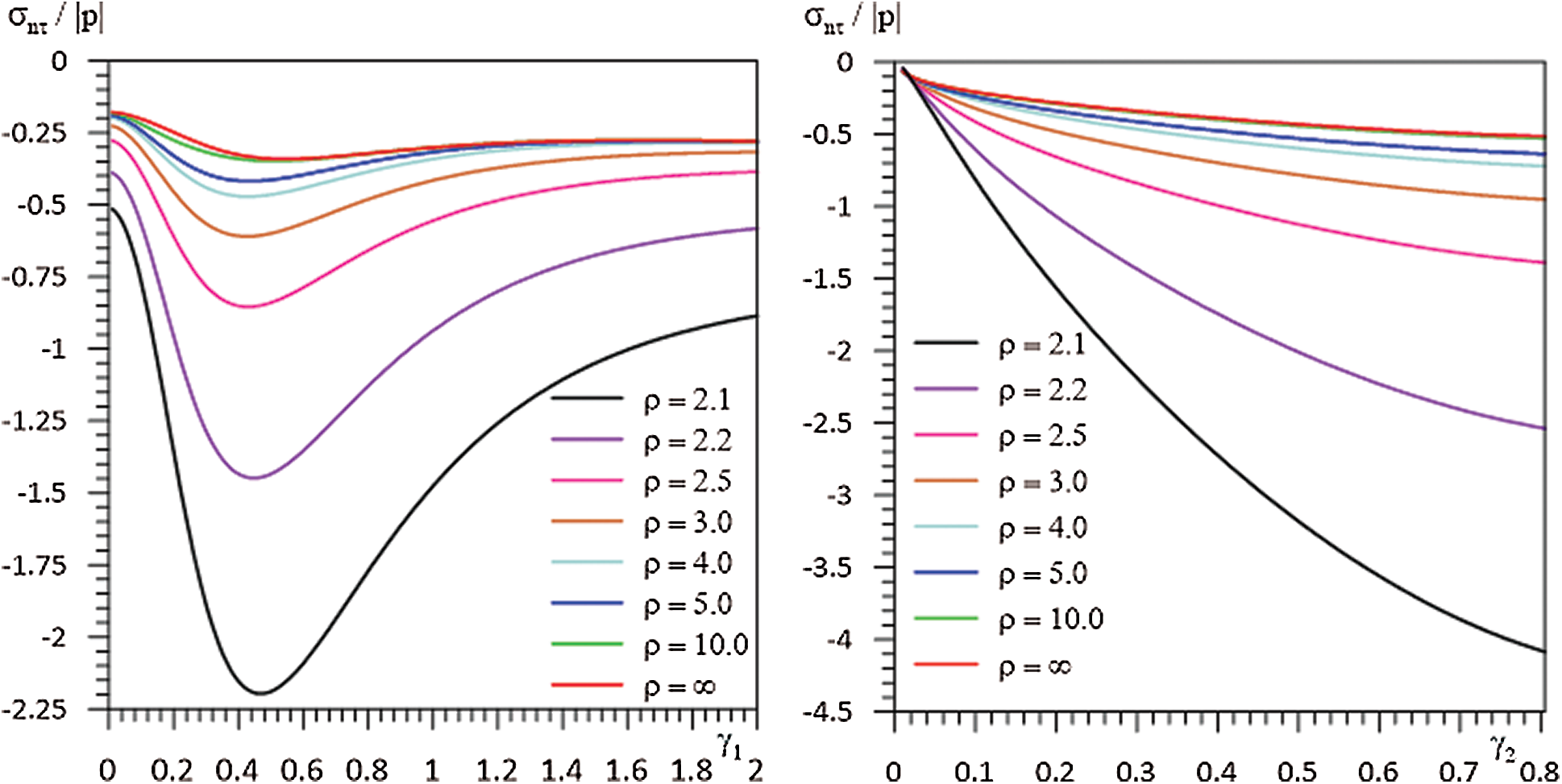
Figure 2: The graph of dependencies between Σnn/|p| and (a) γ1 (γ2=0.3) (b) γ2 (γ1=0.5) for various values of ρ for the case where E=50,ε=0.015

images

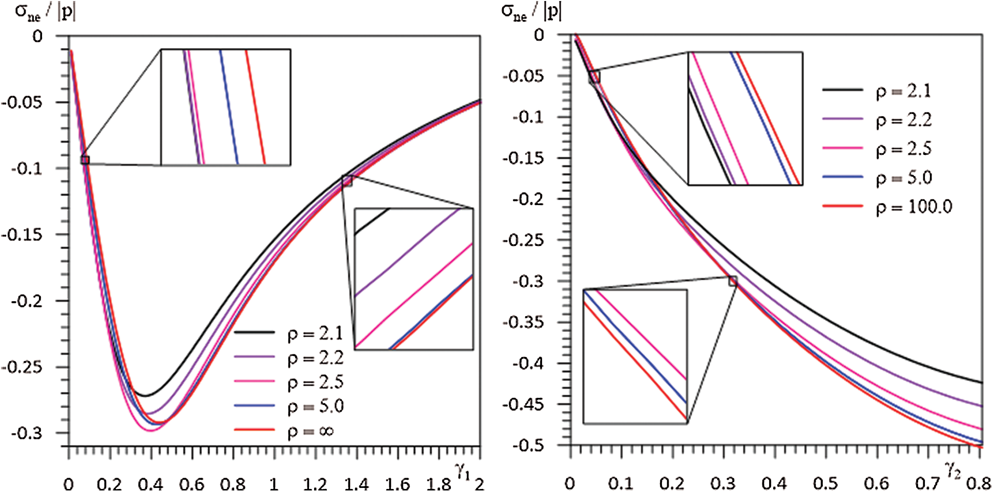
Figure 3: The graph of dependencies between Σnτ/|p| and (a) γ1 (γ2=0.3) (b) γ2 (γ1=0.5) for various values of ρ for the case where E=50,ε=0.015

images

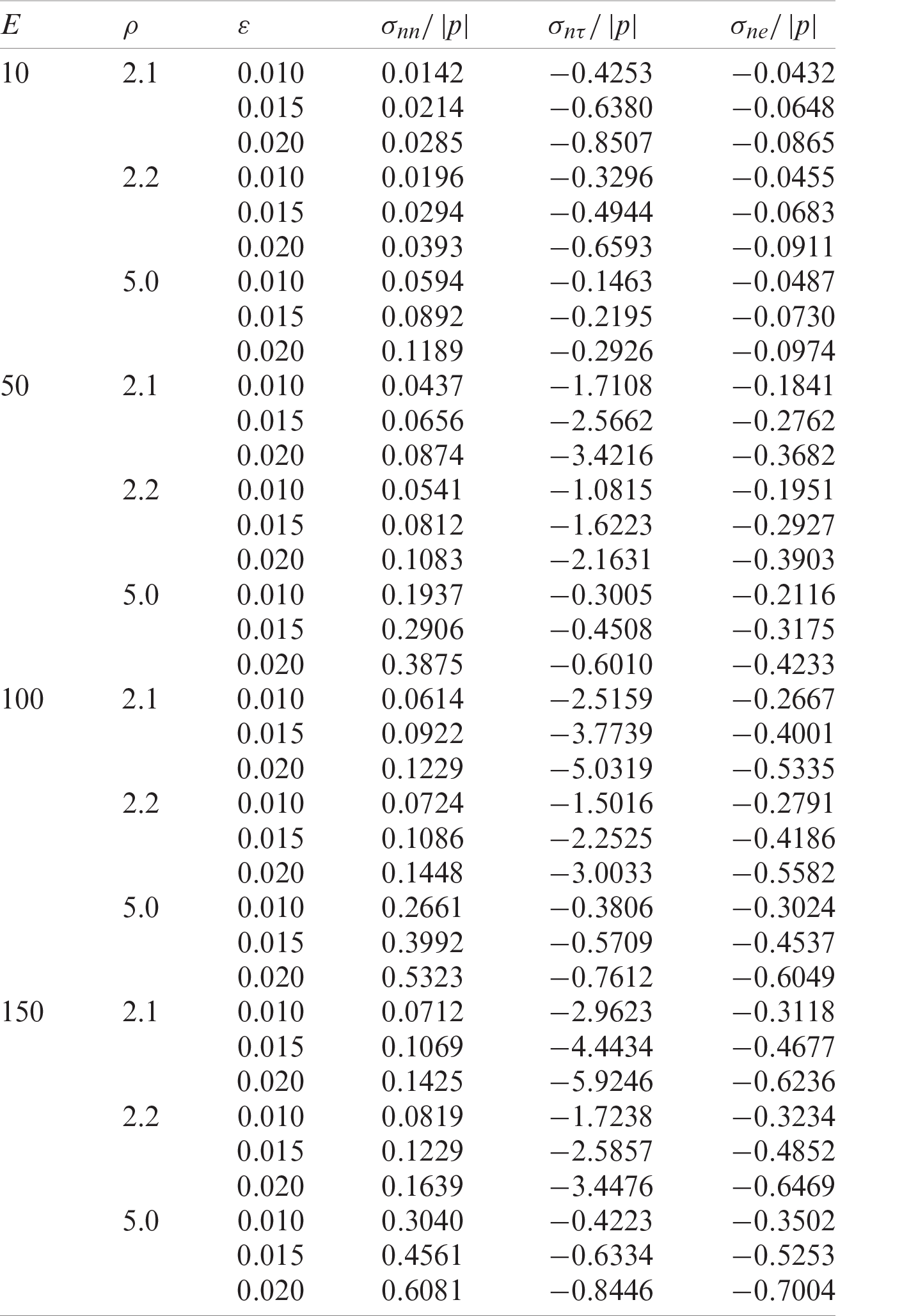
Figure 4: The graph of dependencies between Σne/|p| and (a) γ1 (γ2=0.3) (b) γ2 (γ1=0.5) for various values of ρ for the case where E=50,ε=0.015

Table 1: The stresses in γ1=0.6,γ2=0.4 and various E, ρ, ε

images

In Figs. 2–4, the dependencies between σnn/|p|, σnτ/|p|, σne/|p| and γ1(a), γ2(b), respectively are given where E=50 and ε=0.015, and γ2=0.3 in (a) and γ1=0.5 in (b). According to Figs. 2 and 3, as the hollow fibers approach each other, the values of σnτ/|p| are increasing, but the absolute values of σnn/|p| are decreasing. Although the relationship between the absolute values of these stresses and fiber thickness is monotone, the relationship between these values and the outer radius of the hollow fiber is non monotone. From Fig. 4, it is observed that while the absolute value of σne/|p| increases as the hollow fibers approach each other up to about γ1=0.35, these values then decrease. The same change exists between the fiber thickness and the absolute values of σne/|p|. In this case, the change occurs around γ2=0.12. In addition, it is seen that the σnτ/|p| shear stress values, as absolute values, are higher than the other stress values. According to these results, attention should be paid to the σnτ/|p| shear stress.

With the increase of the distance between the hollow fibers, the interaction between the fibers disappears and thus the same values are reached with the stress values obtained in case [25]. This shows the accuracy of both the algorithms used and the programming made by the authors with the FTN77 programming language.

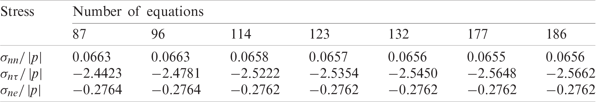
In Tab. 1, the values of σnn/|p|, σnτ/|p| and σne/|p| are given for γ1=0.6,γ2=0.4 and various E, ρ, ε. From this table, it is seen that the values of the stresses are increasing with the parameters ε and E which define the degree of defect and modulus of elasticity ratio, respectively. Also, when γ1=0.6,γ2=0.4, as the hollow fibers approach each other, the values of σnn/|p| and the absolute values of σne/|p| decrease, but the absolute values of σnτ/|p| increase.

Tab. 2 shows how the values of the stresses converge with the number of equations where E=50,γ1=0.6,γ2=0.4,ρ=2.1,ε=0.015. From this, it is seen that 186 equations are sufficient for convergence, and therefore, all values are calculated according to this number of equations.

Table 2: Convergence of the values of the stresses with the number of equations where E=50,γ1=0.6,γ2=0.4,ρ=2.1,ε=0.015

images

5 Conclusions

In this study, the normal and shear stresses at the fiber-matrix interface are studied in the case of two neighboring hollow fibers with infinite length (at least ten times the bending amplitude) with the same phase periodic curvature embedded in an infinite elastic medium. It is thought that the object in question has uniformly distributed normal forces acting along the hollow fibers at infinity, and the midlines which pass through the centers of the fibers have the same plane and phase curvature. The case in which the thicknesses and outer radii of the fibers are the same and where these values do not change along the fibers is discussed. The hollow fibers may be close to each other, but they do not come into contact. The research has been carried out using the piecewise-homogeneous body model and the three-dimensional geometric linear exact equations of elasticity theory. Thus, it is aimed to obtain better quality results than the numerical results obtained using approximate theories.

Within the framework of the above assumptions, the governing field equations provided separately in the hollow fibers and in the matrix are written in accordance with the piecewise-homogeneous body model. Added to these are the conditions provided by the inner surfaces of the fibers and the ideal contact conditions provided at the surfaces where the fibers come into contact with the matrix. Thus, the problem has been formulated as a boundary-value problem which has been solved by using the boundary form perturbation method. According to this method, all expressions related to the surface equations, hollow fibers and matrix are serialized in terms of the small parameter defining the bending degree of the fibers. When these series are used in the governing field equations and boundary conditions, the boundary-value problems provided separately for each approach are obtained. Naturally, the k-th boundary-value problem includes the magnitudes of the previous boundary value problems. Numerical results have been obtained by solving the boundary value problems of the zeroth and first approach. Since the solution of the boundary value problems belonging to the next approaches will affect the numerical results only quantitatively, and not qualitatively, the solutions up to the first approach are considered to be sufficient. With some simple assumptions, the boundary-value problem of the zeroth approach can be solved analytically, while the solution of the boundary-value problem of the first approach is brought to the infinite system of algebraic equations. It has been shown that this infinite system of algebraic equations can be replaced by a finite one by using the convergence criterion. Numerical results are produced by taking a sufficient number of equations according to this criterion.

The obtained numerical results consist of the calculations made at the points where the normal stress of σnn and the values of σnτ and σne shear stresses are maximum. Dimensionless parameters related to the distance between the hollow fibers, the ratio of elasticity constants and fiber bending amplitude are defined, and the effects of these parameters on the stresses are discussed. Accordingly, the following conclusions have been made:

• The relationship between the σnn normal stress and the inner radius of the hollow fibers is non-monotone. In addition, as the fibers approach each other, the values of the σnn normal stress decrease.

• The relationship between the σnτ shear stress and the inner radius of the hollow fibers is also non-monotone. However, as the fibers approach each other, the absolute values of the σnτ shear stress increase. This increase is remarkable.

• The relationship between the σne shear stress and the inner radius of the hollow fibers is also non-monotone. However, the approach of the hollow fibers to each other increases the absolute values of these stress values up to a certain value of the inner radius of the fiber and decreases after this value.

• The relationship between the stresses under consideration and the thickness of the hollow fibers is monotone.

• The increase in the bending degree and in the ratio of elasticity constants increases the values of the stresses as absolute values.

• The numerical results obtained when the distance between the hollow fibers is increased so that there is no interaction between them, coincides with those obtained in [25]. In addition, the numerical results obtained by taking the inner space of fibers to zero are consistent with the results of [12], in which problem the fibers are filled. This demonstrates the accuracy of the numerical results.

The numerical results obtained should be taken into account in the production of materials which have the properties discussed here, when used as structural elements. In addition, for certain values of the parameters (given in [24]), instead of hollow fibers, carbon nanotubes can be considered, and stress distribution and stability problems can be examined.

Funding Statement: This research has been supported by Yildiz Technical University Scientific Research Projects Coordination Department. Project Number: 2014-07-03-DOP01.

Conflicts of Interest: The authors declare that they have no conflicts of interest to report regarding the present study.

References

1. M. O. Seydibeyoglu, A. K. Mohanty and M. Misra, Fiber Technology for Fiber-Reinforced Composites. Cambridge, United Kingdom: Woodhead Publishing, 2017. [Google Scholar]

2. R. P. Tomic, A. Sedmak, D. M. Catic, M. V. Milos and Z. Stefanovic, “Thermal stress analysis of a fiber-epoxy composite material,” Thermal Science, vol. 15, no. 2, pp. 559–563, 2011. [Google Scholar]

3. A. Ahmed and L. Xu, “Numerical analysis of the electrospinning process for fabrication of composite fibers,” Thermal Science, vol. 24, no. 4, pp. 2377–2383, 2020. [Google Scholar]

4. A. Kelly, “Composite materials: Impediments do wider use and some suggestions to overcome these,” in Proc. Book ECCM-8, Naples-Italy, vol. I, pp. 15–18, 1998. [Google Scholar]

5. S. D. Akbarov and A. N. Guz, Mechanics of Curved Composites. Dortrecht, Boston, London: Kluwer Academic Publishers, 2000. [Google Scholar]

6. A. N. Guz, “On one two-level model in the mesomechanics of compression fracture of Cracked Composites,” International Applied Mechanics, vol. 39, no. 3, pp. 74–285, 2003. [Google Scholar]

7. H. T. Corten, “Fracture of reinforcing plastics,” in Modern Composite Materials, L. J. Broutman, R. H. Krock (Eds.Reading, Massachusetts: Addison-Wesley, pp. 27–100, 1967. [Google Scholar]

8. Yu. M. Tarnopolsky and A. V. Rose, Special Feature of Design of Parts Fabricated from Reinforced Plastics. Riga: Zinatne, 1969. [Google Scholar]

9. M. Yu. Kashtalyan, “On deformation of ceramic cracked matrix cross-ply composites laminates,” International Applied Mechanics, vol. 41, no. 1, pp. 37–47, 2005. [Google Scholar]

10. S. D. Akbarov, Stability Loss and Buckling Delamination: Three-Dimensional Linearized Approach for Elastic and Viscoelastic Composites. Berlin, Heidelberg: Springer-Verlag, 2012. [Google Scholar]

11. S. D. Akbarov and A. N. Guz, “Method of solving problems in the mechanics of fiber composites with curved structures,” Soviet Applied Mech March, vol. 20, no. 9, pp. 777–785, 1985. [Google Scholar]

12. R. Kosker and S. D. Akbarov, “Influence of the interaction between two neighbouring periodically curved fibers on the stress distribution in a composite material,” Mechanics of Composite Materials, vol. 39, no. 2, pp. 165–176, 2003. [Google Scholar]

13. S. D. Akbarov and R. Kosker, “On a stress analysis in the infinite elastic body with two neighbouring curved fibers,” Composites Part B: Engineering, vol. 34, no. 2, pp. 143–150, 2003. [Google Scholar]

14. S. D. Akbarov, “Three-dimensional stability loss problems of the viscoelastic composite materials and structural members,” International Applied Mechanics, vol. 43, no. 10, pp. 3–27, 2007. [Google Scholar]

15. S. D. Akbarov, R. Kosker and Y. Ucan, “Stress distribution in an elastic body with a periodically curved row of fibers,” Mechanics of Composite Materials, vol. 40, no. 3, pp. 191–202, 2004. [Google Scholar]

16. S. D. Akbarov, R. Kosker and Y. Ucan, “Stress distribution in a composite material with the row of anti-phase periodically curved fibers,” International Applied Mechanics, vol. 42, no. 4, pp. 86–493, 2006. [Google Scholar]

17. S. D. Akbarov, R. Kosker and Y. Ucan, “The effect of the geometrical non-linearity on the stress distribution in the infinite elastic body with a periodically curved row of fibers,” Computers, Materials & Continua, vol. 17, no. 2, pp. 77–102, 2010. [Google Scholar]

18. S. D. Akbarov, R. Kosker and Y. Ucan, “Influence of the interaction between fibers periodically located in a composite material on the distribution of stresses in it,” Mechanics of Composite Materials, vol. 52, no. 2, pp. 243–256, 2016. [Google Scholar]

19. R. Kosker, “On internal stability loss of a row unidirected periodically located fibers in the visco-elastic matrix,” Thermal Science, vol. 23, no. S1, pp. 427–438, 2019. [Google Scholar]

20. F. Coban Kayıkci and R. Kosker, “Stability analysis of double-walled and triple-walled carbon nanotubes having local curvature,” Archive of Applied Mechanics, vol. 91, pp. 1669–1681, 2021. [Google Scholar]

21. F. Coban Kayıkci and R. Kosker, “Stress distribution in an elastic body with a locally curved double-walled carbon nanotube,” Journal of the Brazilian Society of Mechanical Sciences and Engineering, vol. 43, no. 52, pp. 1–16, 2021. [Google Scholar]

22. R. Kosker and N. Cinar, “Stress distribution in an infinite body containing two neighboring locally curved nanofibers,” Mechanics of Composite Materials, vol. 45, no. 3, pp. 315–330, 2009. [Google Scholar]

23. N. T. Cinar, R. Kosker, S. D. Akbarov and E. Akat, “Stress distribution caused by two neighboring out-of-plane locally cophasally curved fibers in a composite material,” Mechanics of Composite Materials, vol. 46, no. 5, pp. 555–572, 2010. [Google Scholar]

24. S. D. Akbarov, “Microbuckling of a double-walled carbon nanotube embedded in an elastic matrix,” International Journal of Solids and Structures, vol. 50, no. 16–17, pp. 2584–2596, 2013. [Google Scholar]

25. R. Kosker and I. Gulten, “Stress distribution in elastic media containing hollow fiber with periodic curvature,” European Journal of Science and Technology, vol. 19, pp. 809–820, 2020. [Google Scholar]

26. G. N. Watson, A Treatise on the Theory of Bessel Functions. Cambridge: Cambridge University Press, 1966. [Google Scholar]

27. L. V. Kantarovich and V. I. Krilov, Approximate Methods in Advanced Calculus. Moscow: Fizmatgiz, 1962. (in Russian). [Google Scholar]

This work is licensed under a Creative Commons Attribution 4.0 International License, which permits unrestricted use, distribution, and reproduction in any medium, provided the original work is properly cited.