Computers, Materials & Continua DOI:10.32604/cmc.2021.018187
Article

An Optimized Data Fusion Paradigm for WSN Based on Neural Networks

Moath Alsafasfeh1,*, Zaid A. Arida2, Omar A. Saraereh3, Qais Alsafasfeh4 and Salem Alemaishat5

1Department of Computer Engineering, Al-Hussein Bin Talal University, Ma’an, Jordan
2School of Computing and Informatics, Al Hussein Technical University, Amman, 11831, Jordan
3Department of Electrical Engineering, Hashemite University, Zarqa, 13133, Jordan
4Department of Electrical Power and Mechatronics, Tafila Technical University, Tafila, Jordan
5School of Computing and Informatics, Al-Hussein Technical University KHBP, Amman, 11855, Jordan
*Corresponding Author: Moath Alsafasfeh. Email: moath.alsafasfeh@ahu.edu.jo
Received: 28 February 2021; Accepted: 31 March 2021

Abstract: Wireless sensor networks (WSNs) have gotten a lot of attention as useful tools for gathering data. The energy problem has been a fundamental constraint and challenge faced by many WSN applications due to the size and cost constraints of the sensor nodes. This paper proposed a data fusion model based on the back propagation neural network (BPNN) model to address the problem of a large number of invalid or redundant data. Using three layered-based BPNNs and a TEEN threshold, the proposed model describes the cluster structure and filters out unnecessary details. During the information transmission process, the neural network’s output function is used to deal with a large amount of sensing data, where the feature value of sensing data is extracted and transmitted to the sink node. In terms of life cycle, data traffic, and network use, simulation results show that the proposed data fusion model outperforms the traditional TEEN protocol. As a result, the proposed scheme increases the life cycle of the network thereby lowering energy usage and traffic.

Keywords: WSN; clustering; data collection; neural networks

1  Introduction

Sensing technology, wireless communication technology, and embedded computing technology have all advanced in recent years, resulting in the rapid development of low-power, multi-function sensors that can combine data collection, processing, and wireless communication in a small volume [1]. The use of this form of miniature sensor network (Wireless Sensor Network, WSN) has become a crucial part of the Internet of Things (IoT) growth [2]. A wireless sensor network is a multi-hop self-organizing network system made up of a large number of inexpensive miniature sensor nodes placed throughout the detection region. Sensor, sensing object, and observer are the three components of a wireless sensor network [3].

The wireless sensor network (WSN) is a large-scale distributed network of sensor nodes. Its aim is to detect, capture, and process information from sensing objects in the sensor nodes’ deployment area [4]. WSN nodes are often distributed at random, resulting in an unequal distribution of nodes in the monitoring region. The monitoring areas of multiple nodes will overlap as the deployment density increases, resulting in duplication of the sensing data of neighbouring nodes [5]. Sensing data transmission to the sink node alone would waste a lot of communication bandwidth, consume too much energy, and reduce the network’s communication performance, lowering perception data collection efficiency [6]. In response to the aforementioned issues, the use of fusion technology in WSNs will effectively save network resources, improve perception data accuracy, and improve perception data collection efficiency [7]. With the continued advancement of WSNs, an increasing number of researchers have focused on fusing neural networks into WSNs. The optimization of data collection based on mobile sink nodes is currently one of the most important issues in WSN research. The WSN implemented not only a mobile sink node traffic load-balancing node, but also a node that can manage power consumption, effectively avoiding “hot spots” and extending the network’s survival time. However, using mobile sink nodes to collect data introduces new challenges: first, the sink position update problem, where constant flooding of sink location information consumes too much node energy; second, the network topology changes frequently due to sinking movement, which increases the overhead of network topology construction. As a result, academic and application fields have focused on optimising routing protocols based on mobile sink nodes and algorithms for planning mobile sink trajectories. The authors of [8] suggested a fusion approach focused on the use of a rough set and neural network combination. Rough sets are used to simplify network input, reduce the amount of data that the network processes, and improve the network’s training speed. However, the accuracy of the original decision table is critical to this process, and an incorrect original decision table would result in incorrect fusion results. The LEECH-F clustering algorithm is combined with a neural network by the authors in [9]. The cluster structure does not change after the cluster is created, which reduces the energy consumption of each round of sensor network clustering, but it ignores the cluster. The issue of header parameter handover wastes the network’s local resources. The authors of [10] use genetic algorithms to optimise the weights and thresholds of the neural network, which increases the network’s data collection accuracy to some degree, but the algorithm’s limited processing scale and low stability are issues. The authors of [11] use neural networks to interpret the wireless sensor network’s signal changes in order to assess if there is an emergency, but the network’s energy resource limitation is not taken into account when it is built. The authors implemented a self-organizing mapping network in the routing decision of the wireless sensor network in [12], which effectively improved the neural network’s training performance, but this approach has high network hardware requirements and a limited application range.

To address the aforementioned issues, this paper proposes the Balance Privacy-Preserving Data Aggregation BPDA model, which is a WSN data fusion model focused on TEEN clustering and BP neural networks. The TEEN clustering protocol is used by the BPDA model to build a cluster structure in the wireless sensor network. The cluster head selection now includes TEEN threshold control. In the cluster structure information transmission, the BP neural network is used to fuse the sensing data. Via the cluster head, the eigenvalues are sent to the sink node. The related parameters of the BPDA model are moved to the next cluster head when the cluster head is replaced.

2  Network Clustering Based on TEEN Protocol

The BPDA model necessitates the use of a specific clustering routing protocol by the wireless sensor network. The TEEN clustering protocol [13] is used in this article. Fig. 1 portrays the TEEN network model. The TEEN protocol is based on the LEACH protocol, and its clustering approach is exactly the same as the LEACH protocol [14]: the cluster head is chosen regularly and with equal probability, and the non-cluster head nodes join the corresponding cluster nearby, except that in TEEN, after the protocol re-establishes the cluster region each time, the cluster head must broadcast. The TEEN protocol applies a hard threshold (HT) and a soft threshold (ST) to the data transmission, unlike the standard LEACH protocol [15]. The absolute threshold of the controlled data’s characteristic value is referred to as the hard threshold. The node transmitter will send the data to the cluster head when the characteristic value controlled by the node reaches the absolute threshold. The soft threshold refers to the tracked characteristic value’s small-range shift threshold. The node transmitter is activated to report data to the cluster head when the change of the characteristic value is greater than or equal to the change threshold. The parameter value that the user is interested in is the characteristic value, which is manually set by the user. HT & ST processing refers to the method of combining hard and soft threshold processing to produce a characteristic value. The HT & ST protocol is as follows: Next, the sensor node receives sensing data from the outside world on a continuous basis. The node will start the transmitter to send the characteristic value in the next time slot when the characteristic value of the sensing data crosses the hard threshold for the first time. This characteristic value, also known as the sensing value (SV), is saved in the node’s external variable. Following the completion of the first transmission, the next data transmission will begin if and only if two conditions are met simultaneously: the current characteristic value is greater than the hard threshold, and the difference between the characteristic value and the SV is greater than or equal to the soft threshold. Fig. 2 illustrates the operation.

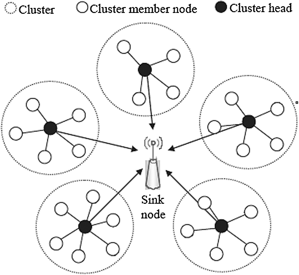
Figure 1: Network model of the TEEN protocol

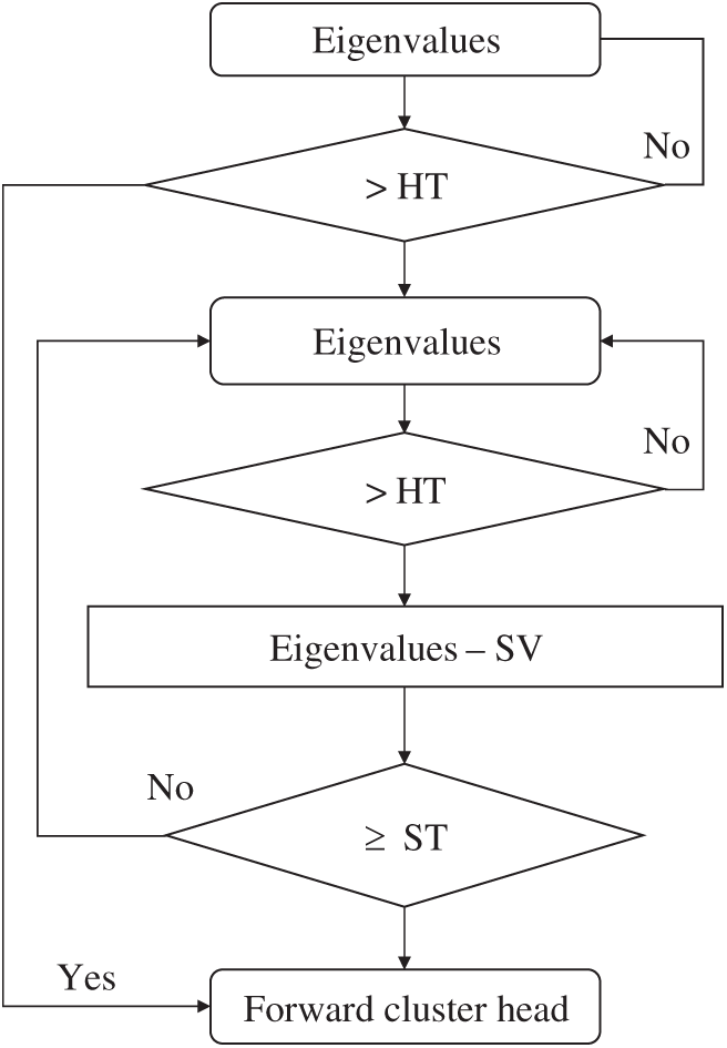
Figure 2: Proposed HT & ST algorithm

The addition of hard thresholds to the network will allow it to filter out unnecessary data based on demand, reducing the amount of data transmitted over the network. Soft thresholds may be used to avoid the transmission of perception data with minimal modification. The network avoids unwanted data transmission, purposefully transmits data that is of interest to users, and with large improvements, thanks to the control of double thresholds.

2.1 WSN Model

In this paper, there are S sensor nodes in the wireless sensor network N, and each node is represented by sn(n=1,2,…,S), N has the following characteristics:

a) The sink node is a one-of-a-kind device that is placed outside of the sensing field. Both sensor and sink nodes can communicate with one another, and the sink node has an endless supply of energy.

b) The sensor nodes are placed in the sensing region at random, and after that, they are set. The sensor nodes’ initial energy is the same, and the energy cannot be replenished. The node dies after the energy is absorbed, and all sensor nodes are identical.

c) The communication channel between nodes consumes the same amount of energy.

d) In the data transmission process, the TDMA method is used.

2.2 Cluster Establishment

Each node in the wireless sensor network is assigned a random number when the cluster head is chosen. If the number generated by the node is less than the threshold T(n), the node sends a message to the surrounding nodes that it is the cluster head. The threshold T(n) is expressed as

T(n)=p1−p∗[rmod (1p)]n∈G(1)

where p is the probability of the election cluster head being elected, usually set to 5% [16]; r represents the current number of rounds in the election cycle; n represents a node; G is a collection of nodes that have not been elected cluster heads before round r. In each cluster construction process, assuming that there are k cluster heads elected in each round, the expression for calculating p is

p=kS(2)

After running 1p round, it means that all nodes have been elected as cluster heads, and 1p round is a fusion cycle of the BPDA model.

2.3 Improved Cluster Head Election Algorithm

After completing a cluster structure calculation, any node can be elected as the cluster head since the TEEN protocol has a high level of randomness in the selection of cluster heads [17]. If the wireless sensor network’s node with the least amount of energy is elected, it will hasten the death of nodes due to energy depletion, reducing the network’s service life. This paper proposes a cluster head selection algorithm based on the residual energy influence factor in light of the TEEN algorithm’s unequal distribution of cluster heads (RECH). In the first round of TEEN protocol clustering, since the sensor nodes have the same energy, the default TEEN clustering algorithm will be used. When the TEEN protocol progresses to the second round, because the energy consumption of each sensor node is different, the previous round of energy consumption must be eliminated because a large number of nodes reduces the probability of a successful election. The selection formula of the RECH algorithm threshold T(n) is as follows

T(n)={p1−p∗[rmod (1p)]n=1pE1−p∗[rmod (1p)]n∈(1,G](3)

where E denotes the influence factor.

Nodes send election messages with different influence factors in the same cluster structure, and the influence factors of nodes in the second round are calculated according to the following expression:

E=max(p+erenew,M)(4)

where p is the probability of TEEN cluster head being elected; er is the remaining energy of the node at the beginning of the current round; enew is the initial node energy value; M is a constant. The value of M is set to 10−4 in this article according to different application settings [18]. The proposed RECH algorithm has a certain enhancement in the clustering speed. The remaining energy in the cluster is introduced into the algorithm, and the selected cluster head is more representative of the cluster members, making the energy consumption of the entire network more balanced.

3  Data Fusion Model Based on Neural Network

3.1 Model Structure

The BPDA model describes a cluster structure in a wireless sensor network using a three-layer BP neural network. Fig. 3 illustrates the model’s structure. This clustered structure is assumed to have a cluster node for the sake of discussion. The BP neural network that corresponds has m input neurons. The cluster head of the cluster structure corresponds to the neural network’s output node. Let the perceptual data source be Y, and there are n parallel output neurons according to the RECH algorithm.

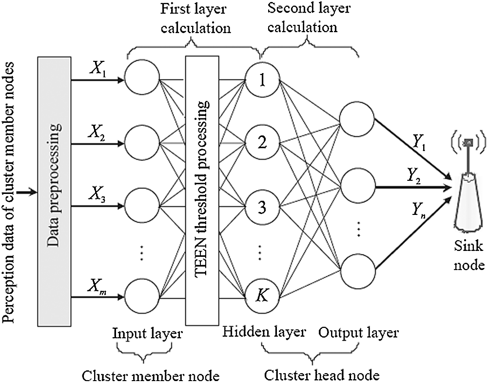
Figure 3: The proposed architecture of the BPDA model

The three-layer BP neural network has been shown in studies to be capable of simulating any nonlinear mapping under the right conditions of the right number of hidden layer nodes and hidden layer layers [19]. There is no relation between nodes in the same layer in the BP neural network. There is an activation mechanism between each layer, and adjacent nodes are linked in pairs. The activation mechanism processes the input of each layer, and the output of each layer is the input of the next layer. In neural networks, there is currently no clear theoretical guidance on the selection of hidden layer nodes. A “trial algorithm” is used in this paper to determine the appropriate number of hidden layer nodes. First, the hidden layer is created using an existing empirical expression for node selection intervals, and then a three-layer BP neural network with variable hidden layers is created, and the influence of the number of hidden layer nodes on network accuracy and network convergence speed is compared using the same experimental sample training to determine the best-hidden layer numeric value.

In the existing empirical expression [20], Eq. (5) can be used as the best reference expression to determine the number of hidden layer nodes

n1=n+m+a(5)

where n1 is the number of hidden layer nodes; m,n denotes the number of output neurons; a is the natural number of (1, 10).

The BPDA model processes information transmission in the cluster structure using a three-layer BP neural network. It filters out unnecessary data using the HT & ST threshold and sends the resulting perception data to the cluster head after the first calculation. The cluster head repeats the second calculation and obtains a set of characteristic values that represent the network data’s characteristics, which it then sends to the sink node.

3.2 Data Fusion Model Based on BP Neural Network

The BPDA model must be initialised after the wireless sensor network has completed clustering and cluster head selection. The initialization of the BPDA model is done in the sink node due to the limited energy of cluster member nodes. The neural network decides certain parameters of itself during the initialization process of the BPDA model, which can be obtained by training, learning, and optimising. The initialization of the BPDA model is also the mechanism of neural network training and learning. The BPDA model first forms a cluster structure in the wireless sensor network using the TEEN clustering protocol, then selects cluster heads using the RECH algorithm. The sensor nodes in this clustering structure accumulate a huge number of sensing data, so the BPDA model normalises the perception data in the cluster member nodes to speed up the fitting of the BP neural network. The linear function conversion approach is used in this article.

y=(Y−minY)(maxY−minY)(6)

where y is the value after preprocessing, Y is the sensor node’s perception data source, minY, and maxY are the minimum and maximum values in the data source, respectively. The TEEN protocol’s HT & ST threshold processing is triggered when normalised perception data enters the neural network’s input layer. Only perception data that passes the HT & ST threshold processing is allowed to reach the first layer of calculation using the BP algorithm. Neuron functions are used to process perception data in the first layer of computation, which is the classification of neurons. Fig. 4 depicts the first layer of measurement logic.

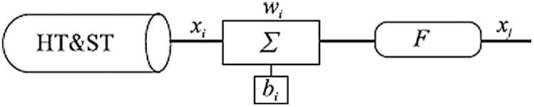
Figure 4: Determination of the first layer of perception data in a neural network

In Fig. 4, wi is the weight of the input neuron; bi is the threshold; F is the activation function, and the activation function processes the output of the input layer. In the first layer of calculation, tansig is selected as the activation function of the network, which is defined as

f(x)=1−e2x1+e−2x(7)

The output of the first layer calculation is xj, which is expressed as

xj=f(∑i=1mwixi−bi)(8)

In the second-layer calculation, the input of the network is the output value of the first-layer calculation. That is, the second-layer calculation and the first-layer calculation of xj belong to the processing calculation of neuron functions. The methods are similar, and this article will not explain in detail. The expression for the output xk of the layer is

xk=f(∑j=1nwjxj−bj)(9)

where wj is the weight of the hidden layer neuron and bj is the threshold. The activation function selected for the second layer calculation is

f(x)=ax+b(10)

where a and b are constants, and the value is related to specific research applications.

After the BPDA model processes the perception data, it forwards the characteristic value xk representing the characteristics of the sample data to the sink node. At this time, the BPDA model pauses the input of the sample and starts to calculate the weight error of the network. The weight error is carried out in two steps. The output errors of the output layer neurons and hidden layer neurons are calculated separately as δk and δj which are expressed as

δk=(ck−xk)xk(1−xk)(11)

δj=∑i=1qδkwjxi(1−xi)(12)

where q is the number of hidden layer nodes and ck is the expected output of the sample. We use the weight error to update the weight threshold of the BP neural network, and the updated weight threshold of the output layer is

wi(N+1)=wi(N)+αδkxi(13)

bi(N+1)=bi(N)+βδj(14)

where α and β are constants, and the value is related to specific application research.

After completing the weight threshold update, the sink node inputs the next sample and cyclically trains until all of the database samples have been completed, completing the BPDA model’s initialization operation. The weights and thresholds of each layer of the neural network have been calculated when the BPDA model completes the initialization process, and the sink node sends these parameters to the corresponding cluster member nodes. These parameters can be used by cluster member nodes to monitor and measure the network’s performance in order to achieve the goal of fusion processing. Since the RECH algorithm selects cluster heads on a regular basis to prevent nodes from dying prematurely due to individual cluster heads’ excessive energy consumption, and because the BPDA model will continuously record relevant parameters and data in order to minimise network energy consumption in the next iteration. As a result, once the next cluster head election is efficient, the BPDA model must transfer the previous iteration’s parameters. When the cluster head is removed, the BPDA model’s parameters are moved. The parameters of the output layer neuron are moved to the new cluster head when the cluster head is replaced. The output layer neuron function is not changed in this article; only the output layer neuron’s weight and threshold are transferred

4  Experiment Analysis

The BPDA model is simulated and evaluated in this paper using the NS-2 network simulation programme [21]. Using real-time temperature monitoring in a wireless sensor network as an example, each sensor node continuously collects the surrounding ambient temperature, and the characteristic value representing the perception data is forwarded from the cluster head to the sink node after the BPDA model’s fusion processing. The experimental results are compared to the TEEN protocol to illustrate the efficacy of the BPDA model, and the actual performance of the BPDA model is measured from three perspectives: the network’s data transmission volume, the number of nodes surviving in the network, and the network’s energy consumption. There are 200 nodes in the simulation system, each with 2 J of energy. The monitoring area is a 100×100 m2 square area and 200 sensor nodes are randomly deployed in the monitoring area. The convergence node is deployed outside the monitoring area. Each evaluation algorithm deploys five different network topologies at random, runs a BPDA model simulation test in each topology, and then averages the five test results as the final simulation test results to avoid the effect of network topology on the experimental results. Each evaluation algorithm deploys five different network topologies at random, runs a BPDA model simulation test in each topology, and then averages the five test results as the final simulation test results to avoid the effect of network topology on the experimental results.

The network traffic is compared in Fig. 5 using the BPDA model and the TEEN clustering algorithm. The amount of contact in this paper is measured by the number of feature values obtained by the sink node. During the sensing data transmission point, the BPDA model dynamically changes the threshold and uses data preprocessing to discard a large number of invalid data packets, compressing the transmission data of the data packets. Fig. 5 shows that the BPDA model can sustain a relatively stable linear growth of contact traffic for approximately 3500 s, while the TEEN protocol can only maintain a relatively stable linear growth for approximately 2500 s. The BPDA model received around 3500 eigenvalues when the experiment hit around 4500s, while the TEEN protocol had received 5000 eigenvalues at about 3800 s, and the BPDA model had less data communication at any time. When the RECH algorithm and the neural network are combined, the BPDA model’s communication volume is greatly increased when compared to the TEEN protocol. As compared to the TEEN protocol, the BPDA model decreases transmission frequency by around 30% when transmitting on the same channel. Next, the BPDA model necessitates less network energy usage, essentially reducing network connectivity and conserving network energy.

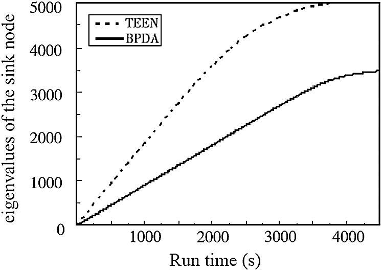
Figure 5: Comparison of data traffic of the proposed and traditional TEEN algorithms

The wireless sensor network relies heavily on sensor nodes operating normally. When a node runs out of energy and dies, the wireless sensor network’s life cycle comes to an end. Under the two algorithms, Fig. 6 depicts the relationship between the number of surviving nodes and time in the network. The death of the first node in the BPDA model is nearly equal to TEEN, both at around 700 s, as seen in Fig. 6, but as the experimental period increases, the death of the entire network node in the BPDA model is postponed for a much longer time than TEEN. The network energy is essentially depleted when the TEEN protocol runs to about 3000 s, while the tBPDA model only exhausts the network energy at about 4200 s. By contrast, the wireless sensor network using the BPDA model has a service life that is approximately 40% longer than the TEEN protocol.

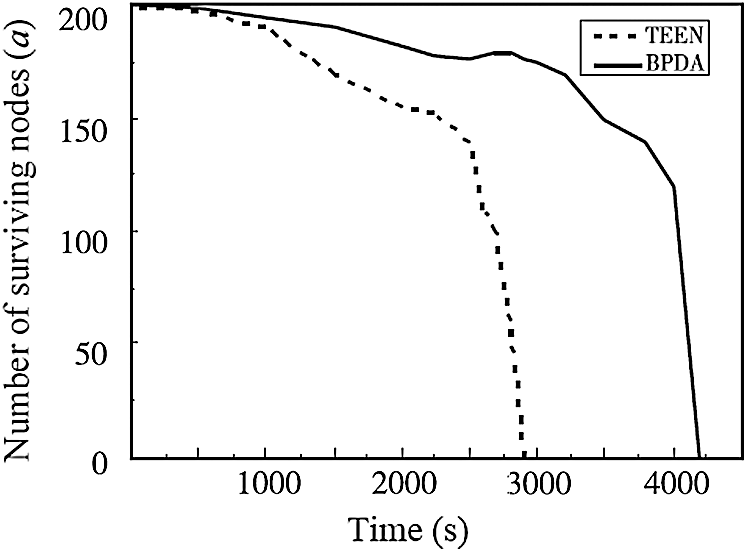
Figure 6: Comparison of the number of survival nodes of the algorithms

The overall energy comparison of the two algorithms is shown in Fig. 7. The network energy increases gradually for a period of time, as shown in Fig. 7, but the energy consumption of the wireless sensor network using the BPDA model is slower. The TEEN protocol seems to have used up all of the network energy around 3000 s, while the BPDA model has used up all of the network energy around 4200 s. When the total number of node deaths from the two approaches exceeds a certain level, the entire network’s energy usage will rise in order to retain the same processing capacity. The BPDA model, as shown in the diagram, can extend the network’s service life and boost its efficiency.

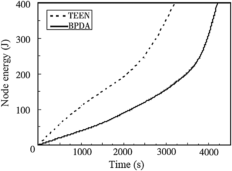
Figure 7: Comparison of the node energy of the algorithms

5  Conclusion

Using a rational clustering structure for data fusion processing will effectively solve the data fusion problem in wireless sensor networks. This paper proposes a TEEN clustering and BP neural network-based data fusion model. The energy impact factor is used in the cluster head selection process so that nodes with more residual energy can be successfully elected. The BP neural network is used in the fusion processing of the sensing data in the cluster structure information interaction phase, and the invalid data packets are discarded by compressing the transmission data of the data packets to achieve the goal of reducing network energy consumption. In comparison to the conventional TEEN protocol, the simulation results show that the BPDA model can significantly reduce network data transmission, reduce network energy consumption, and increase data collection performance. The next step will be to consider other significant WSN considerations, enforce the scheme, and conduct assessment and analysis.

Acknowledgement: The authors would like to thank the editors and reviewers for their review and recommendations.

Funding Statement: The authors have no specific funding for this study.

Conflicts of Interest: The authors declare that they have no conflicts of interest to report regarding the present study.

This work is licensed under a Creative Commons Attribution 4.0 International License, which permits unrestricted use, distribution, and reproduction in any medium, provided the original work is properly cited.