Computers, Materials & Continua DOI:10.32604/cmc.2021.018231
Article

Hybrid BWO-IACO Algorithm for Cluster Based Routing in Wireless Sensor Networks

R. Punithavathi1, Chinnarao Kurangi2, S. P. Balamurugan3, Irina V. Pustokhina4, Denis A. Pustokhin5 and K. Shankar6,*

1Department of Information Technology, M. Kumarasamy College of Engineering, Karur, 639113, India
2Department of Computer Science, Pondicherry University, Puducherry, 605014, India
3Department of Computer and Information Science, Faculty of Science, Annamalai University, Chidambaram, 608002, India
4Department of Entrepreneurship and Logistics, Plekhanov Russian University of Economics, Moscow, 117997, Russia
5Department of Logistics, State University of Management, Moscow, 109542, Russia
6Department of Computer Applications, Alagappa University, Karaikudi, 630001, India
*Corresponding Author: K. Shankar. Email: drkshankar@ieee.org
Received: 01 March 2021; Accepted: 02 April 2021

Abstract: Wireless Sensor Network (WSN) comprises a massive number of arbitrarily placed sensor nodes that are linked wirelessly to monitor the physical parameters from the target region. As the nodes in WSN operate on inbuilt batteries, the energy depletion occurs after certain rounds of operation and thereby results in reduced network lifetime. To enhance energy efficiency and network longevity, clustering and routing techniques are commonly employed in WSN. This paper presents a novel black widow optimization (BWO) with improved ant colony optimization (IACO) algorithm (BWO-IACO) for cluster based routing in WSN. The proposed BWO-IACO algorithm involves BWO based clustering process to elect an optimal set of cluster heads (CHs). The BWO algorithm derives a fitness function (FF) using five input parameters like residual energy (RE), inter-cluster distance, intra-cluster distance, node degree (ND), and node centrality. In addition, IACO based routing process is involved for route selection in inter-cluster communication. The IACO algorithm incorporates the concepts of traditional ACO algorithm with krill herd algorithm (KHA). The IACO algorithm utilizes the energy factor to elect an optimal set of routes to BS in the network. The integration of BWO based clustering and IACO based routing techniques considerably helps to improve energy efficiency and network lifetime. The presented BWO-IACO algorithm has been simulated using MATLAB and the results are examined under varying aspects. A wide range of comparative analysis makes sure the betterment of the BWO-IACO algorithm over all the other compared techniques.

Keywords: Clustering; routing; wireless sensor network; energy efficiency; black widow optimization

1  Introduction

Recently, Wireless Sensor Networks (WSNs) are a significant research topic since they are intended to be applied in extensive domains relevant to ecological observation, emergency response, security tracking in both rural and urban areas especially in hostile regions [1–3]. In general, WSN is comprised of massive, minimum energized intelligent sensors with maximum power sink or base station (BS), which is applicable in making paths between themselves with specific transmission strategies [4]. Also, wireless sensors are highly beneficial because of the simple deployment, self-identification, and time awareness for coordinating with alternate sensors and create dynamic self-organized system. However, it can be firmly constrained with minimum power, storage space, analytical and processing capability, small data rate, and limited range for wireless radio communication [5]. Routing is one of the potential issues to be considered in WSNs. Conventional routing protocols are not applicable for sensor networks directly due to the heterogeneity of networks from ad hoc networks by means of the applied factors like battery-defined sensors, lightweight routing protocols as well as adaptive communication patterns [6]. Fig. 1 shows the structure of WSN.

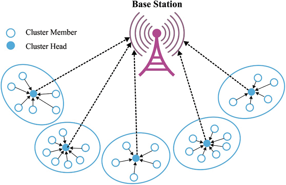
Figure 1: The structure of WSN

Clustering is another important and well-known mechanism used for energy consumption process. In order to develop a clustering approach, the system is classified as massive groups named clusters. Each cluster is comprised of a leader called Cluster Head (CH). Among the clusters, CH is used to gathered data from the member sensors. Moreover, CH computes data collection and eliminates the repeated data and limits the power dispersion of WSN. But, CH intakes maximum power because of the excess overload to receive and collect the data and send them to BS. An important goal of WSN is to influences the routing process in terms of power efficient methods. Therefore, an appropriate CH election is extremely significant for preserving energy and enhances the lifespan of WSN. Then, CH election is assumed to be the optimization issues named as NP-hard. Particle Swarm Optimization (PSO) belongs to the Swarm Intelligence (SI) relied on optimization approach that is an effective mechanism for CH election because of the simple execution, global search, capability to escape from local optima as well as rapid convergence for globally optimal solution.

Moreover, the model of routing protocol is resistant to prominent path interruptions formed by node failure as well as collision. Few routing protocols identify the routing path however, it fails in data communication and tends to reduce the reliability. This problem can be resolved by developing productive multipath routing protocol which activates the data transmission paths among source and BS. As a result, when a path is damaged, the data can be sent through neighboring paths. In additionally, the delivery ratio is increased with reduced latency of the system. Obviously, developers have concentrated to use multipath routing to accomplish consistent data transmission and minimize the control overhead for route identification and enhance the throughput of a network. For developing the closer optimal communication path from BS and sensors, it has to begin route discovery approach used for selecting next hop node which depends upon the topological infrastructure as well as Quality of service (QoS) measures of adjacent nodes. When any event exists, source sensor sends the information to BS by numerous optimal-case multipath within the limited time period by applying Round-Robin Paths Selection model that’s been used for distributes the traffic overload. Consequently, the newly developed routing protocol provides considerable data throughput at the time of reducing packet loss with lower delay and maximize the network lifespan.

This paper presents a novel black widow optimization (BWO) with improved ant colony optimization (IACO) algorithm (BWO-IACO) for cluster based routing in WSN. The proposed BWO-IACO algorithm includes BWO based clustering process to choose an optimal set of CHs. Moreover, IACO based routing process is utilized to select routes for inter-cluster communication. The IACO algorithm combines the ideas of traditional ACO algorithm with krill herd algorithm (KHA). The IACO algorithm exploits the energy factor to select an optimal set of routes to BS in the network. A detailed experimental analysis is carried out to validate the betterment of the BWO-IACO algorithm.

2  Literature Review

Morsy et al. [7] proposed a Gravitational Search Algorithm (GSA) to identify best CHs from collective nodes. Here, node’s Residual Energy (RE) is adopted for CH election. The objectives assumed in CH election are power efficacy, intra cluster distance as well as distance to BS (DBS). Also, single hop technology is applied for sending data from the sensor node and CH. Followed by, multi hop scheme is applied for selecting next hop relied on the cost function to send data through WSN. Moreover, cost function of multi hop scheme assumes RE of next hop and the DBS. Lalwani et al. [8] projected a Harmony Search Algorithm (HSA) for clustering the network and develop the route in WSN. The Fitness Functions (FF) utilized are Node Degree (ND), power, intra-cluster distance as well as distance from CH and sink mode. Hence, power utilization of the node can be limited by deciding the node having reduced distance for data communication.

Lalwani et al. [9] applied a Biogeography Based Optimization (BBO) for selecting CH by means of FF scores like distance between CHs and sink node, distance from nodes of cluster and RE. Also, BBO is applied for generating best and shortest route among CH and sink. The data packets acknowledged by sink node are enhanced by conserving the RE of sensors. Moreover, RE of the system is reduced when compared with Genetic Algorithm (GA) based routing if the sink node is placed to the network externally. Yogarajan et al. [10] employed Ant Lion Optimization for Clustering (ALOC) approach for enhancing the power effectiveness of the system. Furthermore, FF applied in the ALOC has assumed the RE, count of neighboring nodes, distance among nodes, and distance from node and sink. Next, node having maximum count of fitness is assumed to be CH. Afterward, the best route from CHs to sink can be attained with the help of discrete ant LO mechanism. Ezhilarasi et al. [11] established Evolutionary Multipath Energy-Efficient Routing (EMEER) protocol in WSN. Here, Cuckoo Search (CS) model has clustered the network according to the similarity as well as power-level features.

Sirdeshpande et al. [12] implied the Fractional lion (FLION) clustering scheme for generating the optimal routing path in WSN. The FF of FLION model is assumed to be 5 objectives like inter and intra cluster distance, power of CH, normal nodes, and latency. The robust CH election using FLION method is applied for enhancing the network duration. Followed by, FLION clustering scheme does not consider the ND in clustering approach. Arjunan et al. [13] utilized a Fuzzy Logic (FL) to generate unequal clustering as well as ACO for routing among the nodes. Then, nodes are clustered and CHs are decided under the application of FL assumed by means of RE, DBS, distance to neighbors, ND, and node centrality. The cluster maintenance state is applied in WSN used for consuming equal amount of power by CHs. As a result, lifetime of WSN is enhanced significantly. Also, data transmission rate is reduced as the newly developed model is processed in proactive as well as reactive manner.

3  The Proposed BWO-IACO Algorithm

The workflow involved in the presented BWO-IACO algorithm is neatly illustrated in Fig. 2. Consider a set of ‘n’ sensor nodes which are arbitrarily placed in the target region. Then, the initialization of the nodes takes place to collect details related to the adjacent nodes in the network, which are then utilized for clustering and routing processes. Followed by, the BS executes the BWO technique for determining the optimal set of CHs. Once the nodes are aware of becoming CHs, they advertise the status to their neighbors and the nearby nodes join the CH to form clusters. Next to cluster construction, the CMs sense the surroundings and transmitting the data to CHs which needs to forward the data to BS. At that point, the IACO algorithm gets executed to determine the optimal set of routes to BS. Finally, the data will be transmitted from CMs to BS via the chosen routes.

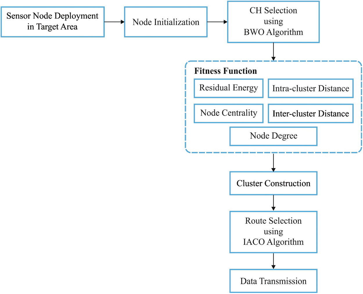
Figure 2: The workflow of BWO-IACO algorithm

3.1 BWO Based CH Selection and Cluster Construction Technique

Similar to Evolutionary Algorithms (EA), the newly developed BWO algorithm are initialized with basic population of spider and each spider denotes the capable solution. The basic spiders are in pairs which manage to recreate the novel offspring. The female black widow consumes the male before or after mating. Followed by, the received sperms are saved and released into egg sacs. Before 11 days of presence laid, spiderlings have emerged from the egg sacs. Then, it cohabits on maternal web for a couple of weeks where time sibling cannibalism has been observed. Fig. 3 illustrates the process involved in BWO method.

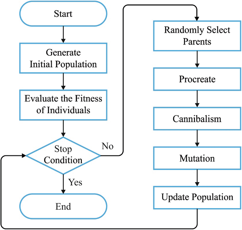
Figure 3: The process involved in BWO algorithm

3.1.1 Initial Population

For resolving the optimization issues, the measures of problem attributes develop proper structure for solution of recent problem. In GA as well as PSO methods, the structure is named “Chromosome” and “Particle position,” correspondingly; however, in BWO model it can be referred as “widow.” In BWO, the capable solution for every problem is assumed to be the Black widow spider. Here, the benchmark functions can be resolved, the structure has to be assumed as the array. In Nvar-dimensional optimization issues, widow is assumed to be an array of 1×Nvar which represents the problem solution. Hence, the array is illustrated in the following:

The variable measures of (x1,x2,xNvar) is a floating-point value. Then, fitness of widow has been accomplished by estimation of FFf at a widow of (x1,x2,…,xNvar). Thus,

The optimization method, the candidate widow matrix with the size Npop×Nvar has been produced with initial spider population [14]. Followed by, pairs of parents are elected arbitrarily for computing the producing step by mating where the male BW is consumed by females.

3.1.2 Procreate

Due to the independent nature, it begins to mate and reproduce new generation and a pair of mateson the web, separately from others. Actually, numerous eggs were laid in a mating, however only the strong spider offspring is endured. Then, the reproduction is initialized by an array named alpha which has to be developed when the widow array having random numbers and offspring is reproduced by α utilizing the applied function (Eq. (1)) where x1 and x2 means the parents, y1 and y2 refers the offspring.

{y1=α×x1+(1−α)×x2y2=α×x2+(1−α)×x1(1)

It is repeated for Nvar/2 iterations where the randomly selected values are not repeated. Consequently, children and parents are included in the array and organized by the fitness measures and based on the cannibalism rating, few individuals are included in newly emanated population.

3.1.3 Cannibalism

There are 3 types of cannibalism. An initial one is sexual cannibalism, where the female BW consumes the male partner in mating. Here, both female and male fitness values can be examined. Secondly, sibling cannibalism occurs where the strong spiderlings consume the poor siblings. Here, a cannibalism rating (CR) is allocated with number of survivors to be determined. Finally, the third class of cannibalism is applied where the baby spiders consume the mother. Here, the fitness score is used for determining strong and weak babies.

3.1.4 Mutation

Here, the Mutepop value of individuals is selected in random fashion from the population. A spider is selected randomly and interchanges 2 elements from the array. Mutepop can be determined using mutation rate.

3.1.5 Convergence

Similar to alternate EA algorithms, 3 termination criteria have been assumed namely, (a) previous count of iterations. (b) Monitoring no variation in the fitness score of optimal BW. (c) Accomplishing the specific accuracy level.

3.1.6 Fitness Function of BWO for CH Selection

The FF of BWO has been applied for selecting the best CH from collective sensors. The RE assumed in FF is employed for eliminating the expired node as a CH in clustering. Followed by, distance from the nodes and distance from candidate CH to sink is utilized for selecting the best CH to reduce the power application of the nodes. Also, ND is adopted for CH election with limited count of normal nodes and conserves the node with maximum iterations. The applied FF are defined in the following: The CH computes different operations by gathering the data from common sensor nodes and send the data to sink node. Thus, CH demands maximum power to achieve predefined operations, thus the node with maximum RE is considered as CH. Also, RE (f1) is depicted in applied Eq. (2).

f1=∑i=1m1ECHi(2)

where, the RE of irh CH is ECHi.

Intra-cluster distance shows the distance from general sensor nodes and corresponding CH. The node’s power dispersion has relied on the distance of communication path. The power utilization of node is minimum if the chosen node has minimum broadcast distance from sink node. Hence, distance between normal sensors to CH (f2) is illustrated in Eq. (3).

f2=∑j=1m(∑i=1Ijdis(si,CHj)/Ij)(3)

where the distance from sensor i and CH j is demonstrated as dis(si,CHj) and the count of sensor nodes from CH is depicted as Ij.

Inter-cluster distance describes the distance between CH to sink node. Here, the node’s energy utilization is based on the distance by broadcast path. For example, when BS is placed away from CH, afterward it requires maximum power to data communication [15]. Thus, immediate fall of CH might exist because of the maximum power consumption. Therefore, node with minimum distance from sink node is considered in data communication. Eq. (4) depicts the objective function of distance from CH and sink node BS (f3).

f3=∑i=1mdis(CHj,BS)(4)

where distance among CHj and sink is represented as is(CHj,BS).

ND is determined as the count of sensor nodes from respective CH. A CH with least count of sensors is decided as the CHs with numerous Cluster Member (CM) exhaust the power within the limited time interval. Moreover, ND (f4) is depicted in Eq. (5).

f4=∑i=1mIi(5)

where Ii denotes the count of sensor nodes from CHi

Node centrality (f5) implies the node placed in central position from neighbor nodes which are demonstrated in Eq. (6).

f5=∑i=1m(Σj∈ndist2(i,j))/n(i)Network dimension(6)

where n(i) defines the count of neighboring node of CHi.

A weight measure has been assigned for an objective value. At this point, multiple objectives are modified as single objective function. Hence, weighted measures are δ1, δ2, δ3, δ4, and δ5. Therefore, single objective function is illustrated in Eq. (7).

where, ∑i=15δi=1,δi∈(0,1)(7)

In which, the scores of δ1, δ2, δ3, δ4, and δ5 are 0.35, 0.25, 0.2, 0.1, and 0.1 correspondingly. The δ1 is assumed for considering the RE as maximum priority to eliminate the node error as CH. Followed by, δ2 and δ3 are regardedas 2nd and 3rd priority to find the CH from sink BS with minimum distance that results in reduced power dispersion. Next, 4th priority (δ4) is applied to the ND for CH election with minimum ND. In addition, node centrality is applied as consequent priority δ5 to enhance the nearness from CH and CM.

3.2 IACO Based Route Selection Process

Once the CHs are chosen, the next stage is the selection of optimal routes to BS using IACO technique. In ant colony method, WSN is defined as the undirected graph. Initially, inexistence of basic pheromone results in minimum solving speed as well as maximum consumption, which has influenced the entire function of ant colony model. This problem can be resolved using the improved ant colony method which depends upon Genetic-Ant Colony approach. Therefore, it results in increased interruption in data communication after crossover as well as mutation. An important goal of this model is to define the KH method and enhance the ant colony performance and share the nodes within the directed graph. As a result, the efficacy of the method can be improved and make sure stability. The KH algorithm [16] belongs to the meta-heuristic optimization approach to resolve the optimization issues which depends upon the result of herding the krill swarms to specific biological as well as ecological processes. The time-based location of a krill in 2D space can be selected using 3 major functions provided in the following:

     i)  The movement influenced by alternate krill,

    ii)  Foraging function,

   iii)  Random diffusion.

KH mechanism has applied the Lagrangian method in d-dimensional decision space as shown below (8):

dXidt=Ni+Fi+Di,(8)

where Ni,Fi, and Di denotes the motion enabled by adjacent krill individuals, foraging action as well as random diffusion of ith krill individual, correspondingly.

First of all, the movement influenced by alternate krill individuals have a way of motion αi, which is around processed using target, local, and repulsive effect. In case of a krill individual, the movement is illustrated by,

Nnew=Nmaxαi+ωnNiold,(9)

and Nmax denotes the high induced speed, ωn refers the inertia weight of motion induced from [0, 1], and Niold defines the final induced motion.

In foraging action has been evaluated by 2 major units. Initially, the food position and secondly, alternate one is prior knowledge regarding the food position. In order to ith krill individual, the motion is around devised in the following:

Fi=Vfβi+ωfFiold,(10)

where

βi=βifood+βibest,(11)

and Vf indicates the foraging speed, ωf implies the inertia weight of foraging action from 0 and 1, Fiold defines the final foraging motion.

In physical diffusion of krill, individuals are assumed to be random procedures. It is determined by means of higher diffusion speed as well as random directional vectors. Finally, it is pointed as given below:

Di=Dmaxδ,(12)

where Dmax indicates the greater diffusion speed, and δ depicts anarbitrary directional vector from [−1, 1].

According to the 3 pre-defined movements, diverse parameters of motion in time, position vector of a krill from the interval t to t+Δt has illustrated by applied function:

Xi(t+Δt)=Xi(t)+ΔtdXidt.(13)

It is apparent that Δt is a well-known and reputed attribute and undergoes fine-tuning by means of special real-time engineering optimization issues [17]. It is due to the scale factor available in speed vector. Thus, brief details are provided regarding the 3 major functions.

In general, Node number m and communication range R has been computed. Assume Vi=Φ,i=1,2,…,m, as the collection of recording existing node number and Pi=0 is the node coefficient. Consider dij as the traffic requirement among node i and node j.

Step 1. Endpoint interacts with closer nodes. Here, closer nodes P(k=1,2,…,m) save the count of ending point and upgrade the node’s coefficient.

When do2k is minimum than R, the Pk is allocated as 1 and O2 is assigned with set Vk.

Step 2. Define the number S of nodes thatare capable of communicating directly toinitial point. A basic value of S is 0, and value plus one is do1 k is minimum to the R.

Step 3. Node j interacts with closer node k. If Pj<Pk or Pk=0, the node k upgrades the p and saves count of node j till reaching the adjacent nodes (j=1,2,…,m).

Followed by, the node receives the data regarding routes from node to endpoint. Then, routes are not composed of back haul.

Triggered with food searching process of ant colony is provided in the following: Assume that S is a set as well as s1,s2,…,sm implies the subsets and coverage of S and, a primary moment which is decided; ant has suited arbitrarily from m-subsets, considering the basic details of a subset τij(0)=C. The possibility of ant k transfer from subset i to subset j:

pijk={[τij(t)]α[ηij]β∑t∈allowedt[τit]α[ηit]β,j∈allowedt0,otherwise.(14)

Based on the applied function, t implies the iteration value, k depicts the ID (k=1,2,…,m), and t indicates the iteration value; τij(t) defines the pheromone efficiency from subset i to subset j; ηij illustrates the inspired degree of ant k moved from subset i to subset j. The above-defined parameters are α and β are collection of data developed from the ant’s sports, mimics the relative significance of ants for selecting a future subset. For balancing the power utilization of nodes, enhanced ant colony approach has emerged as the energy factor according to the fundamental ant colony routing approach for identifying the minimum and maximum energy path [18]. Followed by, enhanced possibility from node i to node j is depicted as follows:

pijk={[τij(t)]α[ηij]β[ξij]χ∑t∈allowedt[τit]α[ηit]β[ξit]χ,j∈allowedt0,otherwise.(15)

Under the application of relative factor which implies the normalization of a model in which ξ means the relative energy factor that refers RE of node j classified by basic node power and measured by 1.2. The attributes χ depicts the accumulation of data and simulated data in the procedure of ant’s sports, it reproduces the relative energy application of ants for selecting the upcoming subset.

Subset p is measured and ant terminates the elements which are selected subset with target node; and the end of cycle. Then, the ants to finish a cycle, the pheromone of subsets are modified on the basis of applied functions:

τij(t+1)=(1−ρ)⋅τij(t)+∑k=1mΔτijk,(16)

where, (1−ρ) denotes the attenuation coefficient of a pheromone; and represented as ρ∈[0, 1] to eliminate the collection of data on subset; Lk defines the count of subsets and k elected during this cycle; Q represents the pheromone strength and it has moved the convergence speed to a greater extent.

4  Performance Validation

Tab. 1 and Fig. 4 depicts the energy efficiency analysis of the BWO-IACO model by means of average RE under different rounds.

Table 1: The comparative average residual energy analysis of BWO-IACO algorithm

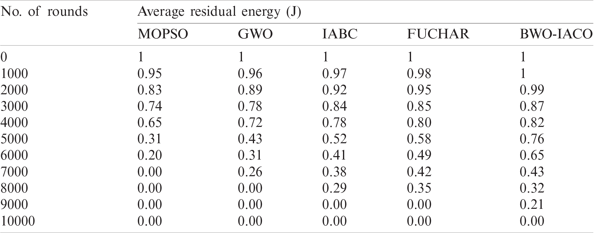
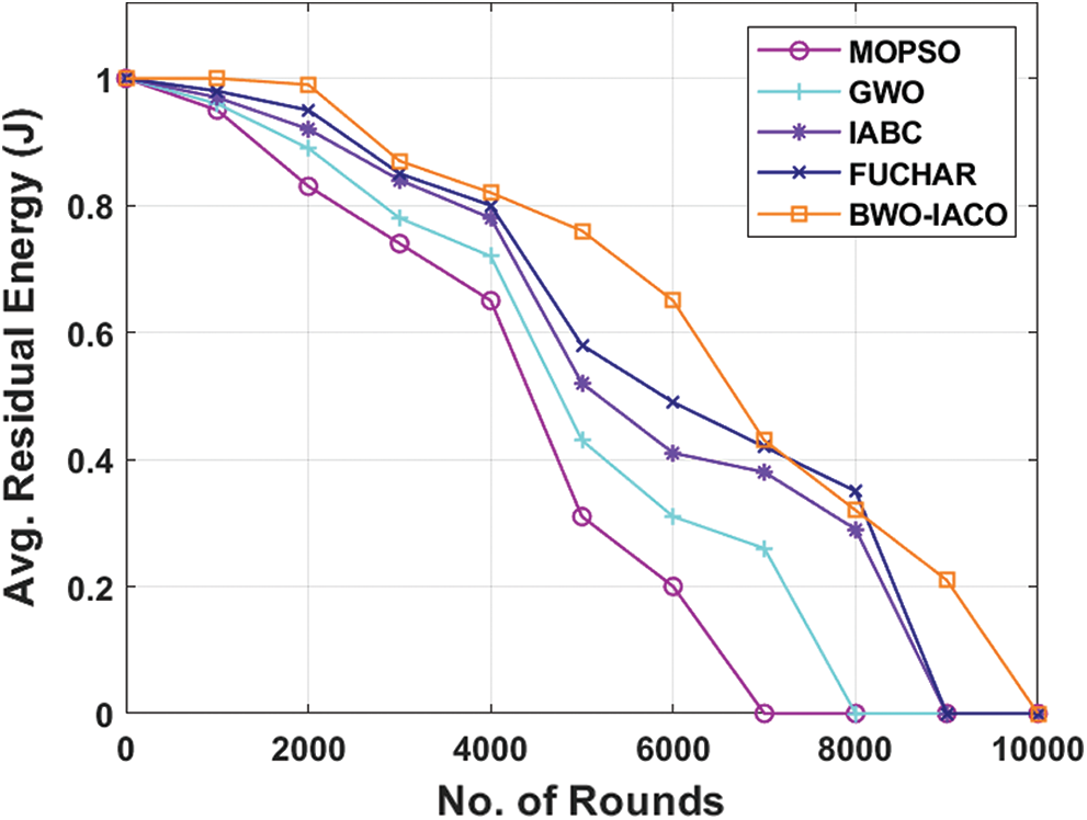
Figure 4: The average residual energy analysis of BWO-IACO algorithm

The figure portrayed that the MOPSO is considered to be poor performer when compared with the earlier models by illustrating higher amount of power consumption. Meanwhile, the GWO has outperformed the MOPSO protocol and accomplished moderate average RE. At the same time, the IABC approach has depicted even better average RE over the previous models. On the other side, the FUCHAR scheme has displayed competing for RE than traditional methods except BWO-IACO model. Finally, the BWO-IACO model has showcased productive performance by reaching high average RE. It portrays that the BWO-IACO framework has consumed minimum amount of power and it gets reduced with an enhancement in number of operating rounds. For example, under the round number of 10000, the MOPSO protocol has drained all power and has average RE of 0J while the GWO, IABC, FUCHAR, and BWO-IACO methodologies have provided a similar result obtaining average RE of 0J.

Tab. 2 and Fig. 5 demonstrated the average delay analysis of BWO-IACO approach under diverse node count. The figure depicted that the MOPSO protocol gains maximum average delay due to single hop communication and random election of CHs. In line with this, the GWO scheme has implied moderate average delay when compared to MOPSO, but not then alternate technologies. Similarly, the IABC framework has illustrated minimum average delay over the conventional algorithms. However, the FUCHAR model has required least and closer identical average delay under diverse node count. But, the BWO-IACO algorithm has represented supreme performance by providing low delay under varying node count. For example, under the node count of 1000, the presented BWO-IACO algorithm acquires the low average delay of 154 ms while the MOPSO, GWO, IABC, and FUCHAR methodologies led to the higher average delay of 239, 211, 195, and 161 ms correspondingly.

Table 2: The comparative average end to end delay analysis of BWO-IACO algorithm

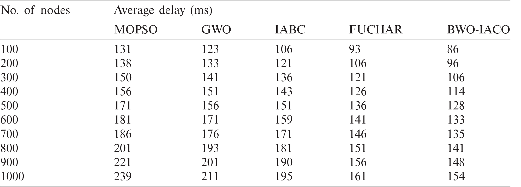
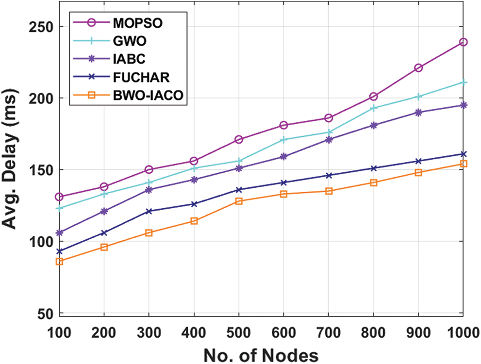
Figure 5: The average delay analysis of BWO-IACO algorithm

Tab. 3 and Figs. 5, 6 illustrates the identification results of the CNNIR-OWELM model on the rice plant disease diagnosis process. On the classification of bacterial leaf blight, the CNNIR-OWELM model has resulted to a higher sensitivity of 0.927, specificity of 0.973, precision of 0.950, accuracy of 0.957, and F-score of 0.938. Similarly, on the classification of Brown Spot, the CNNIR-OWELM method has resulted to a higher sensitivity of 0.865, specificity of 0.936, precision of 0.865, accuracy of 0.913, and F-score of 0.865. Likewise, on the classification of leaf smut, the CNNIR-OWELM model has resulted to a maximum sensitivity of 0.923, specificity of 0.974, precision of 0.947, accuracy of 0.957, and F-score of 0.935. Concurrently, the average analysis of CNNIR-OWELM model has resulted with sensitivity of 0.905, specificity of 0.961, precision of 0.921, accuracy of 0.942, and F-score of 0.913.

Table 3: The comparative packet loss rate analysis of BWO-IACO algorithm

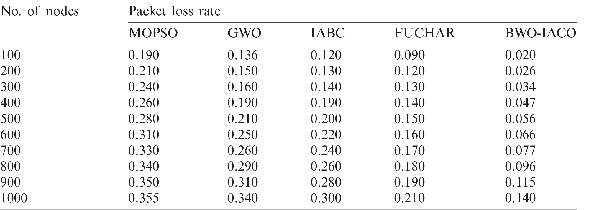
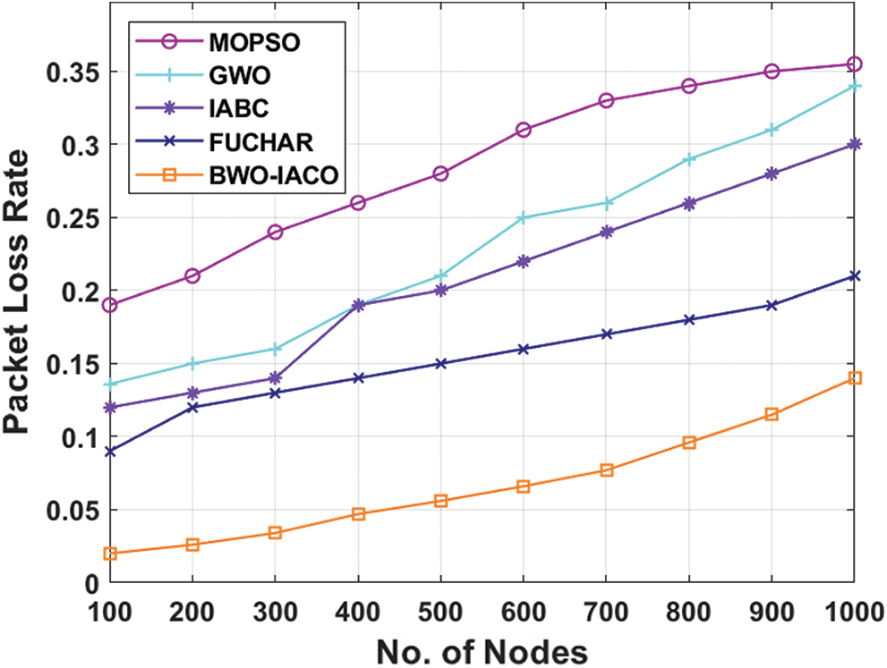
Figure 6: The packet loss rate analysis of BWO-IACO algorithm

Tab. 4 and Fig. 7 inspect the results analysis of the BWO-IACO method with respect to PDR under varying rounds. The figure depicted that the MOPSO is assumed to be poor model and gained less PDR. Also, GWO technology has surpassed the MOPSO protocol and achieved manageable PDR. Simultaneously, the IABC framework has achieved better PDR over the existing models. Then, the FUCHAR algorithm has illustrated acceptable performance over all the other models except BWO-IACO model. At last, the BWO-IACO scheme has attained supreme outcome by reaching greater PDR. It points out that the BWO-IACO scheme has successfully received massive number of packets if related to other models. For example, under the node count of 1000, the MOPSO protocol has obtained low PDR of 0.625 whereas the GWO, IABC, and FUCHAR algorithms have depicted slightly higher PDR of 0.64, 0.68, and 0.77 respectively. Therefore, the presented BWO-IACO method has ensured optimal performance by reaching maximum PDR of 0.84.

Table 4: The comparative PDR analysis of BWO-IACO algorithm

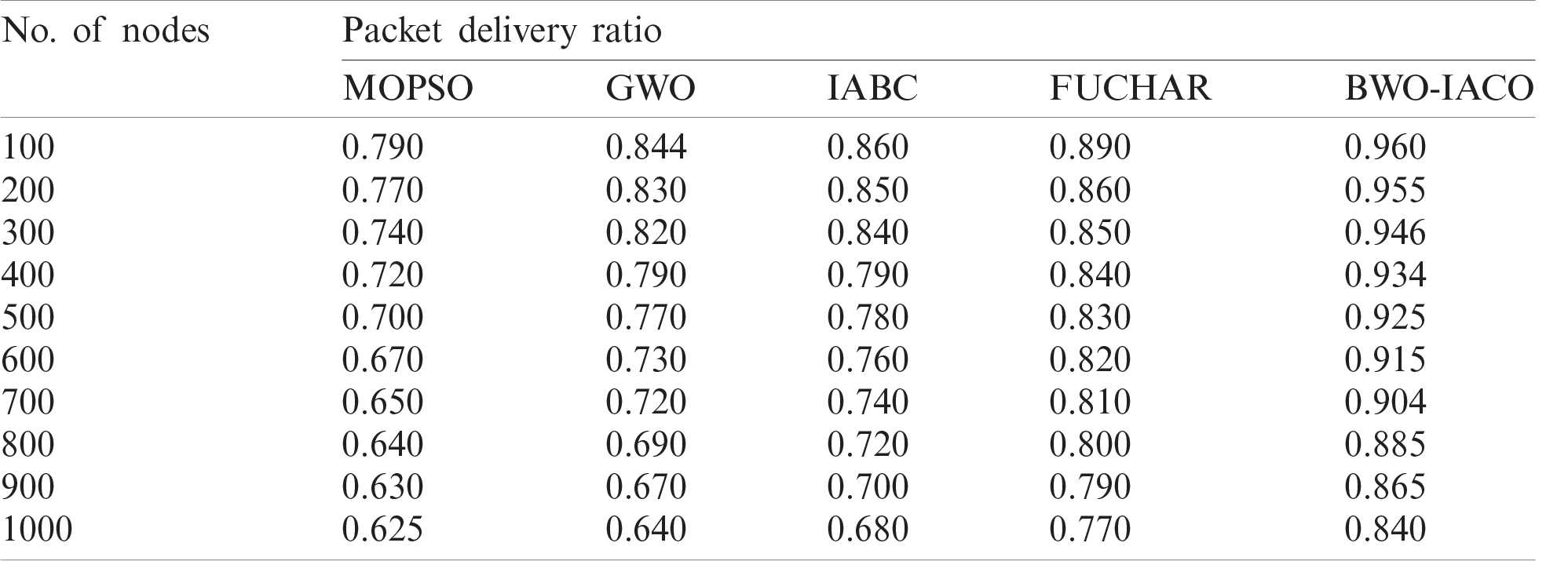
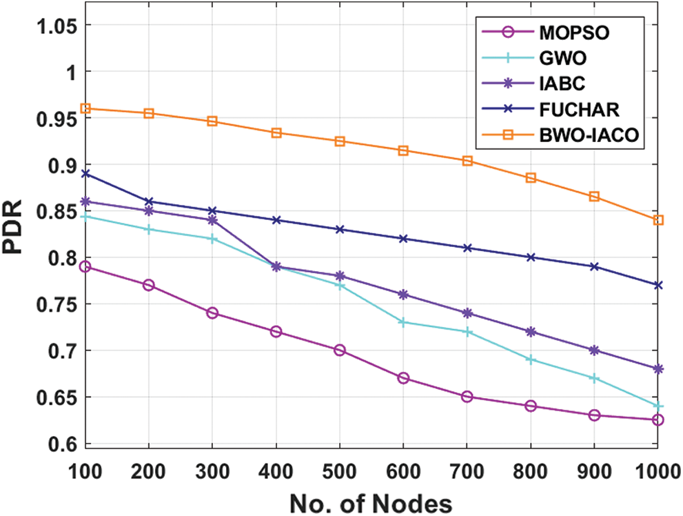
Figure 7: The PDR analysis of BWO-IACO algorithm

Alternatively, the network lifespan is the use of first node die (FND), half node die (HND) and last node die (LND) as depicted in Tab. 5 and Fig. 8. The model which delays the FND, HND, and LND showcases considerable network stability. On determining the network lifetime by means of FND, the MOPSO, GWO, IABC, and FUCHAR technologies led to the FND at the previous rounds. Therefore, the BWO-IACO scheme has delayed the FND to 2198 rounds. Likewise, on computing the network lifetime with respect to HND, the MOPSO, GWO, IABC, and FUCHAR algorithms provided to the HND of 4104, 4514, 5105, and 5594 rounds. But, the BWO-IACO technologies have delayed the HND to 6130 rounds. In line with this, assessing the network lifespan by means of LND, the MOPSO, GWO, IABC, and FUCHAR methodologies resulted in the LND of 6711, 7506, 8129, and 8311 rounds. Thus, the BWO-IACO approach has delayed the LND to 9189 rounds.

Table 5: The network lifetime analysis interms of FND, HND, and LND of BWO-IACO algorithm

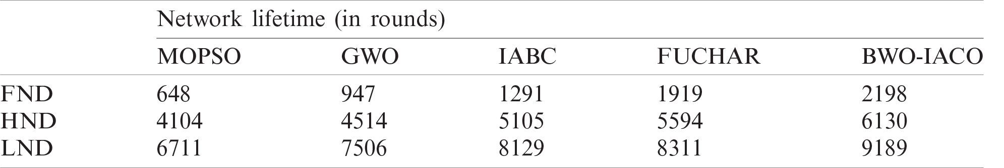
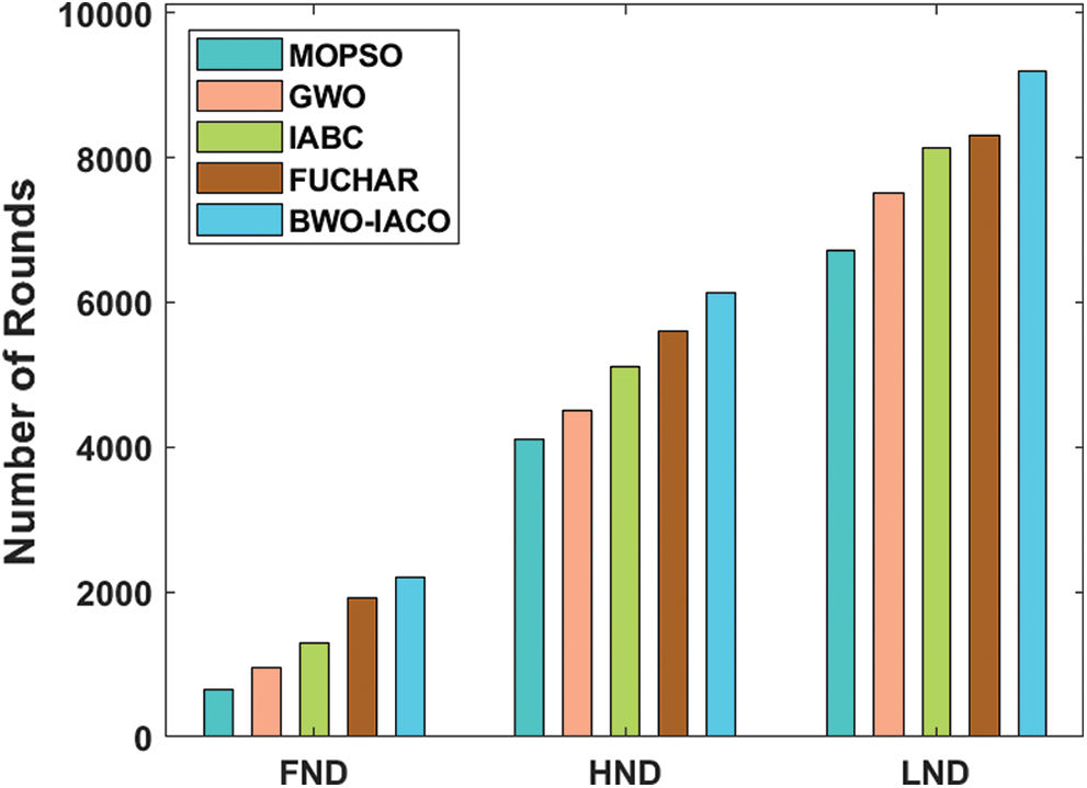
Figure 8: The network lifetime analysis of BWO-IACO algorithm

5  Conclusion

This paper has developed an efficient BWO-IACO for cluster based routing in WSN. The proposed BWO-IACO algorithm makes use of BWO based clustering process with a FF using encompassing five input parameters such as RE, inter-cluster distance, intra-cluster distance, ND, and node centrality. Once the nodes are aware of becoming CHs, they advertise the status to their neighbors and the nearby nodes join the CH to form clusters. Next to that, the IACO based routing process is involved for route selection in inter-cluster communication, which inherits the merits of ACO and KHA. The application of BWO based clustering and IACO based routing techniques significantly improved the energy efficiency and network lifetime. An extensive set of experiments were performed and the comparative analysis makes sure the betterment of the BWO-IACO algorithm over all the other compared techniques. In future, data aggregation and cluster maintenance systems are involved to further extend the network lifetime of WSN.

Funding Statement: The authors received no specific funding for this study.

Conflicts of Interest: The authors declare that they have no conflicts of interest to report regarding the present study.

References

 1.  I. F. Akyildiz, W. Su, Y. Sankarasubramaniam and E. Cayirci, “Wireless sensor networks: A survey,” Computer Networks, vol. 38, no. 4, pp. 393–422, 2002. [Google Scholar]

 2.  K. Romer and F. Mattern, “The design space of wireless sensor networks,” IEEE Wireless Communications, vol. 11, no. 6, pp. 54–61, 2004. [Google Scholar]

 3.  K. Akkaya and M. Younis, “A survey on routing protocols for wireless sensor networks,” Ad Hoc Network, vol. 3, no. 3, pp. 323–349, 2005. [Google Scholar]

 4.  J. Yick, B. Mukherjee and D. Ghosal, “Wireless sensor network survey,” Computer Networks, vol. 52, no. 12, pp. 2292–2330, 2008. [Google Scholar]

 5.  P. Toldan and A. A. Kumar, “Design issues and various routing protocols for wireless sensor networks,” in National Conf. on New Horizons in IT, Mumbai, Maharashtra, India, pp. 65–67, 2013. [Google Scholar]

 6.  L. J. G. Villalba, A. L. S. Orozco, A. T. Cabrera and C. J. B. Abbas, “Routing protocols in wireless sensor networks,” Sensors, vol. 9, no. 11, pp. 8399–8421, 2009. [Google Scholar]

 7.  N. A. Morsy, E. H. AbdelHay and S. S. Kishk, “Proposed energy efficient algorithm for clustering and routing in WSN,” Wireless Personal Communications, vol. 103, no. 3, pp. 2575–2598, 2018. [Google Scholar]

 8.  P. Lalwani, S. Das, H. Banka and C. Kumar, “CRHS: Clustering and routing in wireless sensor networks using harmony search algorithm,” Neural Computing and Applications, vol. 30, no. 2, pp. 639– 659, 2018. [Google Scholar]

 9.  P. Lalwani, H. Banka and C. Kumar, “BERA: A biogeography-based energy saving routing architecture for wireless sensor networks,” Soft Computing, vol. 22, no. 5, pp. 1651–1667, 2018. [Google Scholar]

10. G. Yogarajan and T. Revathi, “Improved cluster based data gathering using ant lion optimization in wireless sensor networks,” Wireless Personal Communications, vol. 98, no. 3, pp. 2711–2731, 2018. [Google Scholar]

11. M. Ezhilarasi and V. Krishnaveni, “An evolutionary multipath energy-efficient routing protocol (EMEER) for network lifetime enhancement in wireless sensor networks,” Soft Computing, vol. 23, no. 18, pp. 8367–8377, 2019. [Google Scholar]

12. N. Sirdeshpande and V. Udupi, “Fractional lion optimization for cluster head-based routing protocol in wireless sensor network,” Journal of the Franklin Institute, vol. 354, no. 11, pp. 4457–4480, 2017. [Google Scholar]

13. S. Arjunan and P. Sujatha, “Lifetime maximization of wireless sensor network using fuzzy based unequal clustering and ACO based routing hybrid protocol,” Applied Intelligence, vol. 48, no. 8, pp. 2229–2246, 2018. [Google Scholar]

14. V. Hayyolalam and A. A. P. Kazem, “Black widow optimization algorithm: A novel meta-heuristic approach for solving engineering optimization problems,” Engineering Applications of Artificial Intelligence, vol. 87, pp. 1–28, 2020. [Google Scholar]

15. P. Maheshwari, A. K. Sharma and K. Verma, “Energy efficient cluster based routing protocol for WSN using butterfly optimization algorithm and ant colony optimization,” Ad Hoc Networks, vol. 110, pp. 1–15, 2021. [Google Scholar]

16. A. H. Gandomi and A. H. Alavi, “Krill Herd: A new bio-inspired optimization algorithm,” Communications in Nonlinear Science and Numerical Simulation, vol. 17, no. 12, pp. 4831–4845, 2012. [Google Scholar]

17. G. Wang, L. Guo, A. H. Gandomi, L. Cao and A. H. Alavi, “Lévy-flight krill herd algorithm,” Mathematical Problems in Engineering, vol. 2013, pp. 1–14, 2013. [Google Scholar]

18. T. Zhi and Z. Hui, “An improved ant colony routing algorithm for WSNs,” Journal of Sensors, vol. 2015, no. 6, pp. 1–4, 2015. [Google Scholar]

This work is licensed under a Creative Commons Attribution 4.0 International License, which permits unrestricted use, distribution, and reproduction in any medium, provided the original work is properly cited.