Computers, Materials & Continua DOI:10.32604/cmc.2021.018389
Article

A Stochastic Flight Problem Simulation to Minimize Cost of Refuelling

Said Ali Hassan1, Khalid Alnowibet2, Miral H. Khodeir1, Prachi Agrawal3, Adel F. Alrasheedi2 and Ali Wagdy Mohamed4,5,*

1Department of Operations Research and Decision Support, Faculty of Computers and Artificial Intelligence, Cairo University, Giza, 12613, Egypt
2Department of Statistics and Operations Research, College of Science, King Saud University, Riyadh, 11451, Kingdom of Saudi Arabia
3Department of Mathematics and Scientific Computing, National Institute of Technology Hamirpur, Himachal Pradesh, 177005, India
4Department of Operations Research, Faculty of Graduate Studies for Statistical Research, Cairo University, Giza, 12613, Egypt
5Wireless Intelligent Networks Center (WINC), School of Engineering and Applied Sciences, Nile University, Giza, Egypt
*Corresponding Author: Ali Wagdy Mohamed. Email: aliwagdy@gmail.com
Received: 06 March 2021; Accepted: 07 April 2021

Abstract: Commercial airline companies are continuously seeking to implement strategies for minimizing costs of fuel for their flight routes as acquiring jet fuel represents a significant part of operating and managing expenses for airline activities. A nonlinear mixed binary mathematical programming model for the airline fuel task is presented to minimize the total cost of refueling in an entire flight route problem. The model is enhanced to include possible discounts in fuel prices, which are performed by adding dummy variables and some restrictive constraints, or by fitting a suitable distribution function that relates prices to purchased quantities. The obtained fuel plan explains exactly the amounts of fuel in gallons to be purchased from each airport considering tankering strategy while minimizing the pertinent cost of the whole flight route. The relation between the amount of extra burnt fuel taken through tinkering strategy and the total flight time is also considered. A case study is introduced for a certain flight rotation in domestic US air transport route. The mathematical model including stepped discounted fuel prices is formulated. The problem has a stochastic nature as the total flight time is a random variable, the stochastic nature of the problem is realistic and more appropriate than the deterministic case. The stochastic style of the problem is simulated by introducing a suitable probability distribution for the flight time duration and generating enough number of runs to mimic the probabilistic real situation. Many similar real application problems are modelled as nonlinear mixed binary ones that are difficult to handle by exact methods. Therefore, metaheuristic approaches are widely used in treating such different optimization tasks. In this paper, a gaining sharing knowledge-based procedure is used to handle the mathematical model. The algorithm basically based on the process of gaining and sharing knowledge throughout the human lifetime. The generated simulation runs of the example are solved using the proposed algorithm, and the resulting distribution outputs for the optimum purchased fuel amounts from each airport and for the total cost and are obtained.

Keywords: Stochastic flight problem; cost of refuelling; ferrying strategy; tankering; discounted prices; simulation procedure; nonlinear mixed binary model; metaheuristic algorithm; gaining-sharing knowledge-based algorithm

1  Introduction

Reference [1] states that the aviation sector connects the world in a special way and contributes 8% to the global economy and aviation’s demand for oil accounts for approximately 12.7% of the transportation sector and industry. Reference [2] shows that at the international level, the international air transport is a very powerful and dynamic sectors, the International Civil Aviation Organization (ICAO) reaches an agreement on the aviation standards in order to obtain a secure, safe and sustainable air operation. Reference [3] shows that at the national level, Airport Consultative Committees with the airport authorities exchange ideas and consult different aspects of the development programs and try to resolve any issues that may emerge.

Reference [4] shows that there are a series of processes for planning flight operations for each season, including scheduling, fleet allocation, routing, and crew scheduling problems. Airlines usually create their plans, that are often interrupted, and the airlines often suffer significant expenses.

Reference [5] shows that the airline companies aim to optimize their operations to meet fuel efficiency objectives, they face challenges as to how to execute efficiency measures in the day-to-day service of the airline and in the various business areas. Optimizing the flight route aims to decrease the influence of the aircraft on the climate across the airport in a method that considers jet noise, fuel consumption, aircraft restrictions and constraints. The flight operations concentrate on developing a system that can help manage the fuel usage.

One of the largest direct operational costs factors in the air transport industry is fuel consumption. Reference [6] predicted that the fuel for a standard A320 family operator, represented between 28–43 percent of the overall operating costs. The fuel crisis in the 1970s aroused great attention to the issue of airline fuel management. Nowadays, the cost of jet fuel has become an increasing proportion of airline expenditures and has changed greatly. Reference [7] shows that the cost of aviation fuel could continue to rise, impacting the financial performance of airlines and the provision of national air service and placing persistent pressure on airlines to sustain positive cash flows.

In a given flight rotation, the aircraft will begin at an airport number 1, then flies to successive airports till finally reaching the last airport and then back to airport number 1. For a specific flight return, the aircraft will begin at airport number 1, then flies to the successive airports till finally reaches the last airport, then the aircraft will return from the last airport to the initial one vice versa.

The fuel for either of these flights may be purchased at the departure or the previous city in the series and “tankerin” for the subsequent flights. So, a fuelling policy can be planned that allows a plane to board fuel for a single leg only or for any number of legs that follow.

Reference [8] shows that the it is very important to reduce cost of purchasing fuel for domestic and foreign air transport routes. In a companion RAND publication, a comprehensive study of fuel saving possibilities can be obtained.

Fuel ferrying or tankering is a strategy of purchasing fuel in excess to cover the next leg of the flight taking into account the extra fuel consumed by flying in excess of the required weight, “tankerin fuel” is the quantity of extra fuel. Tankering will minimize the total cost of fuel by shifting the purchased fuel from expensive to cheaper places. It takes advantage of fluctuations in fuel costs in different cities and country/regions.

The fuel purchased in a certain airport is a function of the minimum amount of fuel needed along each leg of the route in the flight rotation, the maximum carrying capacity of the aircraft and the fuel consumption in such a flight. Regular fuel consumption depends on the minimum amount of fuel carried on the aircraft, whenever this amount exceeds this amount, fuel consumption will increase.

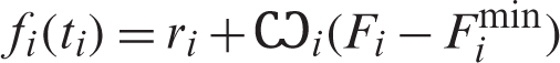
Major airlines believe and adopt the concept of fuel ferrying, they have developed low-cost fueling techniques and forecasting and planning tools to decide if their flights must tanker fuel to lower the operational costs. Fig. 1 demonstrates a fuel-loading diagram scheme along a standard fuel-ferrying technique for an aircraft route. A purchased fuel quantity is loaded at the origin airport with the additional existing ferried fuel. Then, the accumulated amount of fuel will be completely or partially consumed. When ferrying strategy is implemented in airport (i) for example, an extra fuel amount will remain as a “tankerin fuel” when the airplane lands in the following airport (i + 1). When ferrying process is repeated in multiple airports in the flight route, then a multi-stage fuel ferrying strategy is occurred.

1.1 Motivation

In simple practical application problems, two assumptions are considered:

     i)  Fuel price is considered fixed and does not change with the purchased amounts.

    ii)  Variations in flight times are not considered or they are neglected.

In simple cases, the fuel price in each airport is assumed to be fixed and the time duration for each flight leg is considered as deterministic. Such assumptions are not realistic, in more realistic cases, the fuel price can vary as a function of the purchased fuel quantity and the flight time is random in nature. To be more precise, variations in the fuel prices and in time durations should be exactly measured and taken into considerations. The multi-step fuel prices as a function of the purchased fuel amounts and the stochastic version of the flight route problem will be taken into consideration in this study.

2  Literature Review

Many efforts have been made to formulate the fuel allocation problem, the main goal of which is to solve the purchasing amounts that can take full advantage of the current tankering opportunities.

Reference [9] implemented a fuel control and allocation model that specifies the best aircraft refueling strategy. It was used operationally by the National Airlines Fuels Administration and Right Control Departments, resulting in savings of several million dollars. For each flight, the model determined the best fueling station and provider, based on the rate, price, available capacity, fuel consumption, flight data, and tanker cost, the model used also detailed methods for sensitivity analysis.

Reference [10] claimed that the National’s computer-based fuel allocation model in 1976 helped the organization to reduce fuel costs. According to reports, in the first year of using the model, the cost has been reduced by approximately US $3 million. The average computer cost was less than US $300 per month. The inspiration for this heuristic strategy was to develop a linear programming model, which gave remarkable alternatives and proved to be of considerable value.

Reference [11] formulated the task as a network, the model resulted in an increase in energy intensiveness of 1.7 percent occurred when a Boeing 727 on a 250-mile stage ferries 10,000 pounds of fuel. Ferrying fuel during long-distance flights can cause potentially massive problems. An additional carry of 10,000 pounds of fuel on a Boeing 727 will increase energy intensiveness by 0.9% on a 1,500-mile hop. Although the extra amount of fuel required to consuming is nearly 10% of ferried fuel.

Reference [12] specified various variants of the airline refueling issue when there is a restriction in the amounts of fuel obtained from a supplier. He considered a linear function with defined parameters for fuel consumption for each flight. The proposed model is a linear programming one based on fuel costs, fuel station constraints and supplier constraints to minimize the cost of fuel tankering for aircrafts. However, it can be simplified to a pure network problem if there were no station or supplier constraints. If there was either restrictions on fuel stations or suppliers, it can be simplified to a generalized network problem. This model was used by McDonnell Douglas, a major American aerospace company created by the combination of McDonnell Aircraft and the Douglas Aircraft Corporation to evaluate the profit potential for different types of aircraft, with common cost savings of 5 to 6 percent.

The disadvantage of such models is that they neglect the additional cost of extra burning fuel due to heavier fuel weight. In fact, filling the aircraft with higher fuel weight increases the needed maintenance which are not considered in most of the models. Reference [13] proposed a mathematical model with an objective that identifies the optimal fuel ferrying strategies taking into consideration the balance of saving cost and cost of fuel burn and maintenance. A series of tests were carried out to analyze the possible advantages and disadvantages of the suggested ferrying strategy.

Reference [14] discussed existing procedures, models and flight procedure design software used in the commercial industry, especially in collaboration with Atlas Air, Continental Airlines, FedEx and UPS. His paper defines the conditions and requirements that should describe the flight refueling and tankering plan, and is a basic model comparing the fuel costs of historical data with and without ferrying. It indicated that future tankering could save up to 111 million US dollars per year. The document further described the positive and negative aspects that the Air Force needed to consider if such a policy is to be introduced. It also discussed various aspects that should be included in each tanker deployment plan, with a focus on general safety and training, thereby optimizing future savings.

Reference [15] highlighted the problem of aircraft routing and ferrying strategy. The key contribution was to predict maintenance costs while evaluating fuel ferrying techniques. A mathematical model was proposed and expanded to provide three options for fuel costs in a limited hypothetical network of 5 stations and 18 flight segments. The findings demonstrated that shifts and variations in fuel prices enabled the ferrying approach to successfully solve the problem of aircraft routing.

Reference [16] provided a linear programming model to optimize the refueling volume on the route network of Brazilian airlines, where no constraints on the purchasing or storage capacity of each supplier. It was shown that fuel ferrying strategy contributes for 5 per cent economic savings, but creates a 1 percent increased fuel consumption, and a debate on the effect of the environment for this method was also presented.

Reference [17] forecasted future cost savings if the Air Mobility Command (AMC) carry the highest possible fuel. They evaluated the cost of fuel of non-ferried flights in Fiscal Year 2012 with the expected cost of ferried flights. They discussed the changing prospects for possible savings when AMC shifts from war to peace. Under baseline/wartime conditions, fuel tankering would save US $151 million per year, accounting for approximately 2% of the Air Force’s total fuel expenditure of US $8.81 billion in fiscal year 2012. Most of the potential savings made by fuel tankering on C-130, C-17 and C-5 flights were from activities in Afghanistan and Iraq. In Afghanistan, fuel tinkering was used to achieve the highest cost savings by taking advantage of the wide difference between fuel rates inside and outside the operating room, where fuel rates were as high as three times.

Reference [18] considered the problem of optimizing airline ferrying method, the analysis focused on cost. Regression established the relation between flight time and fuel consumption and genetic algorithms were used to solve optimization problems. The mathematical model was applied to 20 scheduled flights to predict their fuel consumption. The optimal fuel scheduling problem was solved in 20 seconds of software runtime, relative to the amount of time typically expended by human effort. The optimized fuel lift plan demonstrated 30% decrease when utilizing the optimized schedule relative to the used one.

3  Cost of Extra Fuel Weight

Reference [19] defines Cost of Weight (COW) as the excess fuel consumed, as a result of extra weight. IATA suggests determining COW as relation between Landing Weights (LW) and the fuel consumption per hour. To calculate COW, it is needed to determine the weight factor of a certain flight in relation to the flight time, (t), then the total extra fuel burned for the full length of a flight = CW factor (TOW) × increase in take-off weight as follows:

where:

ΔW = Weight change,

Weight factor as a function of total flight duration, t.

IATA calculates COW factor according to the (LW) while ignoring the Take-Off Weight (TOW) which should be used where there is tankering. Reference [20] demonstrated a new approach to calculate COW for different flight times in a single step.

Applying Eq. (1), the extra fuel burned in an airline trip from an airport (i) to an airport (i + 1) can be calculated using the following equation:

where:

Δfi= Extra fuel burned in the trip between airports (i) and (i + 1),

ΔWi= Extra weight of fuel carried out over the minimum required amount in the trip between airports (i) and (i + 1),

i= Weight factor for the flight between airports (i) and (i + 1) as a function of the total time.

The regular fuel burned from one airport to another is based on carrying the minimum amount of fuel on this flight. When more amount is carried, the amount of fuel burned will be higher.

The total fuel burned in the flight is thus given by:

where:

ri = regular fuel burned (1000 Gallons) between airports (i) and (i + 1) when carrying the minimum amount of fuel (Fmini),

Fimin= minimum amount of fuel for a flight between airports (i) and (i + 1),

Fi = amount of fuel on board when going from airport (i) to (i + 1).

4  Mathematical Model

Reference [21] shows that the theoretical structure of mathematical modelling activities is believed to be a vital device for representing and solving real life world problems in an optimal way. Mathematical model as a product which enhances the studying process of complex problems faced in real life situations. Reference [22] studied many specific areas in airplane transportation industry, one of the most important is the aviation fuel consumption and refueling. Reference [23] presented a review of various scientific works related to fuel consumption in aviation industry after the oil embargo in 1973. Reference [24] explained six categories of FCO research methodologies for fuel burnt optimization. Reference [25] shows that it is very important to have real and complete data relative to the problem for building a proper mathematical model for the considered problem.

Many factors must be taken into consideration for this to be determined:

1.    The fuel price at each airport in the used route,

2.    The fuel availability at the airport,

3.    The maximum amount of fuel the aircraft type can carry,

4.    The maximum landing weight allowed at an airport,

5.    The fuel remaining on board at the completion of each leg,

6.    The fuel burnt in relation to weight, flight altitude, weather, and speed.

7.    The extra fuel burnt in relation to the flight time,

8.    The time duration of a specific flight which is not deterministic but is a random variable in nature.

The distribution function for the time duration for the flight legs in a complete flight route. Taking into consideration all these factors, the relevant mathematical model is formulated as follows:

4.1 Decision Variables

Let xi = The amount of purchased fuel at airport i, i = 1, 2, …, n = number of airports in the rotation.

4.2 State Variables

Let yi = The amount of ferried fuel (remaining from the previous flight) at airport i, i = 1, 2, …, n.

4.3 Problem Constraints

i) Fuel on Board Constraints:

A fuel on board constraint is an upper or lower bound on the amount of fuel on board at an airport for all flights.

xi+yi≥Fimin,i=1,2,…,n(4)

xi+yi≤Fimax,i=1,2,…,n(5)

where:

Fimin= Minimum required fuel amount for the flight.

Fimax= Maximum allowed fuel amount on board when take-off (leaving) airport i.

ii) Supplier Constraints:

It is an upper limit on the fuel purchased at a specific airport:

xi≤Simax,i=1,2,…,n(6)

where: Simax= maximum allowed amount of fuel at station i.

iii) State Variables Constraints

The price may be much lower at some earlier airports, and it may seem the optimal policy would be to purchase the maximum amount there and tanker the extra fuel through the following legs. However, this may not even be feasible. The extra fuel burnt results then in added consumption for all the following flight legs on which the fuel is tankerin. If it were not taken into consideration, an extra purchase would be necessary later in the rotation, at a much higher cost than at the first station, in order to replace it.

The state variable yi is equal to the amount of fuel on board (remainder from the last flight leg) at airport i, i = 1, 2, …, n-1. The amount of fuel when landing in airport (i + 1), yi+1 can be calculated as the amount of fuel on board at take-off (leaving) the preceding airport (i) minus the fuel burned on that flight.

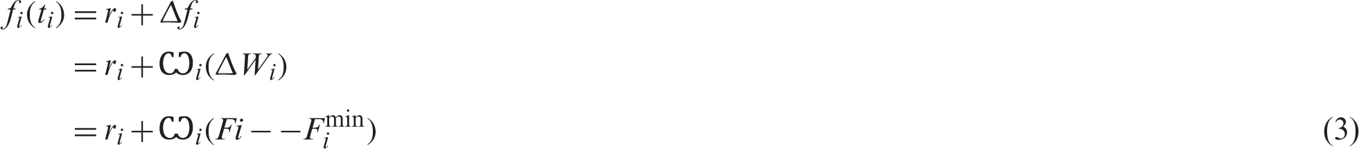
Considering the total fuel burned indicated in Eq. (3):

where: i= Weight factor for the flight between airports (i) and (i + 1),

The amount of fuel remaining on board at airport (i + 1), yi+1 is calculated as follows:

yi+1 equals the amount on board when leaving the preceding airport (i) minus the fuel burned on that flight, fi, then we have:

After rearranging, it will have the form:

y1 is calculated by considering a flight return from the last airport n as the preceding one before the first airport, so, it is calculated as follows:

After rearranging, it will take the form:

iv) Ferried Fuel Bounds:

The Remaining fuel at the airport should not exceed the maximum threshold defined by the company’s operating policy.

yi≤Rimax,i=1,2,…,n(9)

where:

Rimax= maximum allowable landing (ferried) fuel at airport i.

v) Nonnegativity Constraints

All variables

xiandyi≥0,i=1,2,…,n(10)

Fig. 1 represents a simple scheme of the flight rotation problem with n airports, it demonstrates also the decision variables xi, the state variables yi and the fuel burned going from airports (i), (i + 1) and the fuel consumption fi.

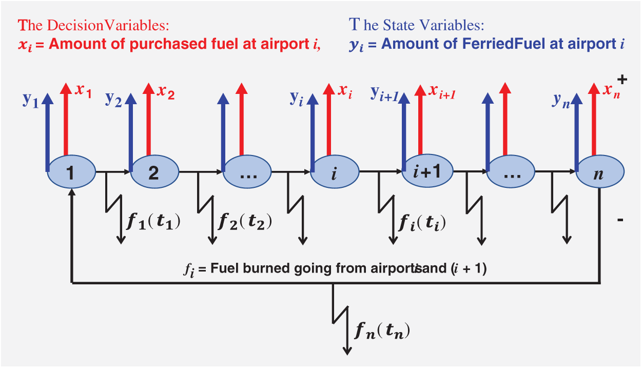
Figure 1: A scheme representing the flight rotation problem

vi) Discounted Prices Constraints

In many cases, the unit price for the purchased fuel is not constant. Consider an airport j where the unit cost has the shape of stepped prices as a function of the amount of purchased fuel xj as shown in Fig. 2 drawn for a number of nj stepped prices. To formulate such a case, the corresponding decision variable xj is substituted with a set of nonnegative decision variables xjr representing the purchased amount of fuel at airport j with unit prices =pjr, r = 1, 2, …, Nj = number of steps of unit prices at airport j, j = 1, 2, …, nj = number of airports with discounted unit prices as shown in Fig. 3. The stepped prices are as follows:

pjr for purchased quantities Fjr-1<xjr≤Fjr, r = 1, 2, …, Nj,

Where Fjr= Upper pound of the discounted unit price pjr.

The set of discounted unit prices are expressed in detail as follows:

pj1 for purchased quantities xj1, 0 ≤xj1<Fj1,

pj2 for purchased quantities xj2, Fj1≤xj2<Fj2,

Figure 2: A scheme representing the discounted prices problem

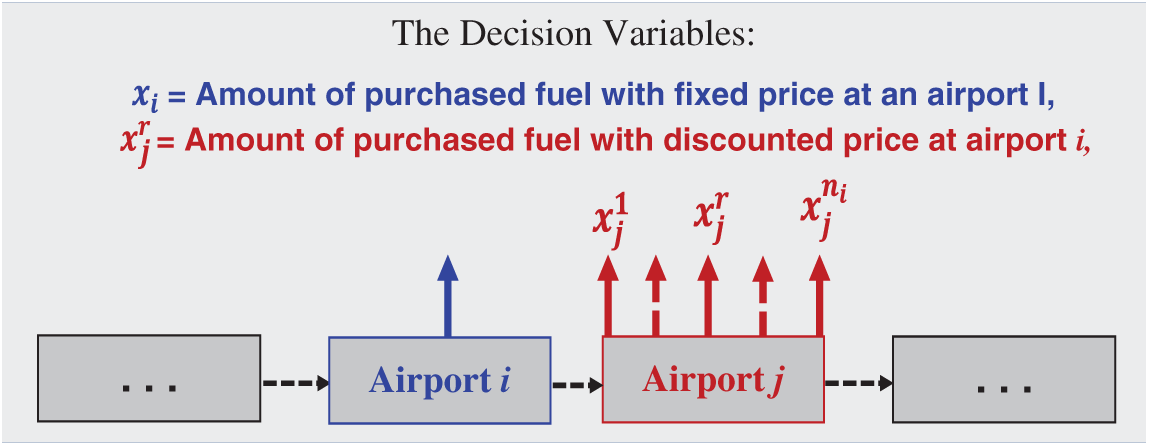
Figure 3: Decision variables for a discounted prices airport

pjr for purchased quantities xjr, Fjr-1≤xjr<Fjr, …,

pjNj for purchased quantities xjNj, FjNj-1≤xjNj<FjNj

For each j = 1, 2, …, nj, it is needed that at most one from all the corresponding decision variables xjr, r = 1, 2, …, Nj be positive, this is achieved by introducing a set of dummy binary variables as follows:

For each j = 1, 2, …, nj, it is needed that at most one from all the corresponding decision variables xjr, r = 1, 2, …, Nj be positive, this is achieved by introducing a set of dummy binary variables as explained in the following section.

Dummy Variables

Let a dummy variable djr= 0 or 1, j = 1, 2, …, nj, r = 1, 2, …, Nj.

Consider the following set of discounted prices constraints:

xjr≥Fjr-1.djr,r=2,3,…,Nj,(11)

xjr≤Fjr.djr,r=1,2,…,Nj,(12)

∑r=1Njdjr≤1,(13)

djr=0or1,j=1,2,…,njandr=1,2,…,Nj(14)

Each constraint r in the set of constraints (11) and (12) force the corresponding decision variable xjr to obey the lower and upper bounds. Constraint (13) will satisfy the condition that at most one of the dummy variables djr= 1 while all the others = 0. Accordingly, at most one of the decision variables xjr can take the value 1 arbitrarily which will be determined by the minimization of the objective function.

The calculation of the state variables in Eqs. (7) and (8) will be updated for any airport j that applies a discounted prices strategy by replacing the corresponding decision variable xj with the summation (∑r=1Njxjr) as follows:

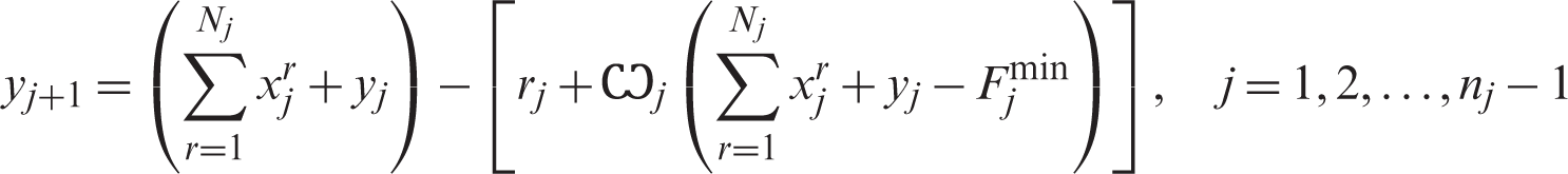
After rearranging, it will have the form:

If the last airport n has a stepped fuel prices, then y1 is calculated by considering a flight return from the last airport n as the preceding one before the first airport, so, it is calculated as follows:

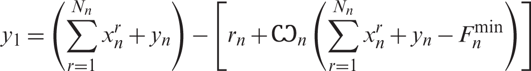
After rearranging, it will have the form:

The objective function will take the form:

MinimizeZ=(∑i=1nipixi)+(∑j=1nj∑r=1Njpjr.xjr)(17)

where: ni = Number of airports without price discounts,

nj = Number of airports with price discounts, and

n = ni + nj.

Another way to deal with the discounted fuel prices is to represent the furl price as a function of the purchased quantities whenever possible. This method is suitable when it is possible to indicate the price as a function of the purchased quantities with a fair goodness of fit. So for an air port j with discounted prices, define pi = fj(xj), where fj(xj) is a nonlinear function representing the relation between the unit cost of fuel with respect to the quantity xj of the purchased quantities from the corresponding airport j.

In this formulation, no need then to introduce the dummy variables nor to the corresponding constraints (11)–(14). The objective function in this case will have the form:

MinimizeZ=∑i=1nipixi+∑j=1njfj(xj)xj(18)

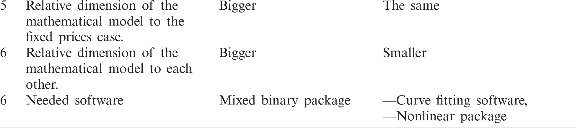
Tab. 1 represents a brief comparison between the two methods for dealing with price discounts schemes (dummy variables and curve fitting methods).

Table 1: Comparison of methods for handling discounted fuel prices

5  A Flight Rotation Case Study

An anonymized airline company is searching minimizing the cost of refuelling by considering ferrying strategy. A plane starts the route in Atlanta, to Los Angeles, then to Houston, to New Orleans, and returns to Atlanta where the route repeats again. Reference [26] shows the flight rotation and the average fuel cost in various places in the United States as presented in Fig. 4.

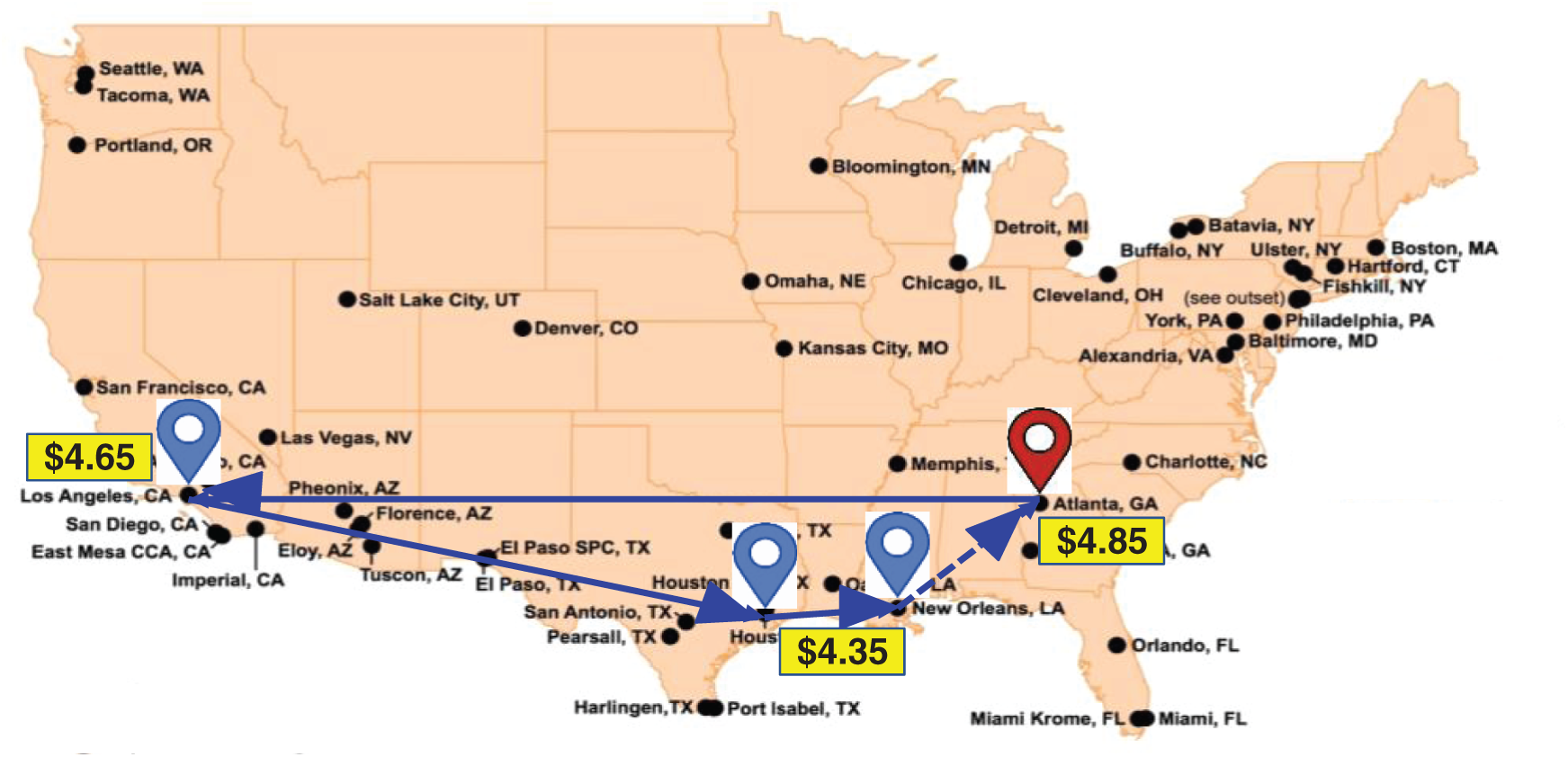
Figure 4: The flight rotation and the fuel costs for the case study

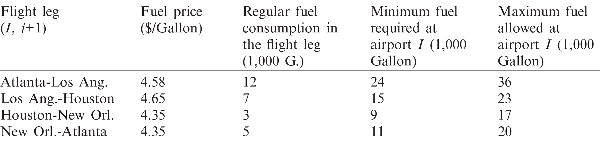
Reference [27] shows the input data include the aircraft flight rotation schedule, regular fuel consumption by flight leg, fuel prices at different airports, availability and restrictions by vendor, the maximum and minimum fuel weight limits for take-off and the maximum fuel weights for landing, this information is provided in Tab. 2. For more than the minimum amount of fuel the fuel consumption is increased due to excess fuel consumption.

Table 2: Data for the flight rotation case study

The top management at Los Angeles airport found that the purchased amount of fuel is very little, they decided to try increasing their market share by price discounting. They are reduced 10% and 20% when the amount of fuel reaches 3,000 and 6,000 Gallons respectively. The decision variable for Los Angeles xL is replaced with a set of 3 nonnegative decision variables xL1, xL2 and xL3 with unit prices 4.650, 4.185 and 3.720 respectively. Reference [28] illustrates the Cost of Wight (COW) factor for the A330-200 data as shown in Fig. 5, based on Take Off Weight (TOW), compared to the one based on Landing Weight (LW) for the full length of a flight. Reference [29] software package that demonstrates the equation of COW (TOW) for the plotted points using an appropriate computer fitting. The best fitted equation for the COW(TOW), (t) is a symmetrical sigmoidal in the form:

y=d+a-d1+(xc)b, where: a = –0.3535106, b = 0.8686458, c = 725188700 and d = 5035722.

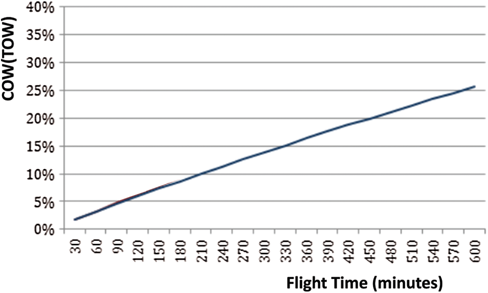
Figure 5: Cost of weight factor

Applying the symmetrical sigmoidal equation, the cost of weight factor for an airport i as a function of total flight time (ti) will be given as follows:

where: ti = total flight time between airports (i) and (i + 1)

Reference [29] is used to interpolate the stepped discounted prices. The computer program fails to interpolate a suitable equation for three steps shape, guided by an optimum solution obtained using the dummy variables, the first step in discounting is not used. Fig. 6 presents the interpolation for both the cost of weight factor and the stepped discounted prices. The best fitted nonlinear symmetrical sigmoidal equation with a satisfactory R2 = 0.94 is:

fj(xj) = 3.759346 + (4.658566 – 3.759346)/ [1 +(xj/5.998055)1104.572]

The curve fitting equation is substituted in the objective function as follows:

Minimize Z = 4.58xA +{3.759346 + (4.65856 – 3.759346) / [1 +(xL/5.998055)1104.572]}. xL + 4.35xH + 4.35xN

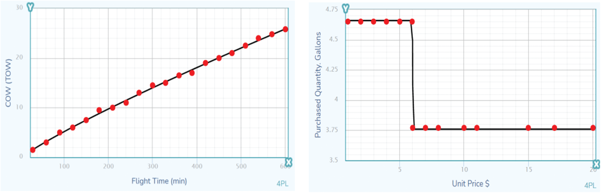
Figure 6: The output screens of the interpolation

6  Stochastic Flight Route Problem

The PDF for flight time is continuous with two bounds. Reference [30] shows that it is suitable to choose the Beta distribution to represent the flight time. Reference [31] shows that Beta Distribution is used when the corresponding variable has an interval, the most popular is the activity times in project management.

The PDF of Beta distribution is:

The Beta Function is:

Reference [32] shows that three-time estimates (a), (m) and (b) are used in PERT method, and it has been a usual tool for probabilistic activities durations. The three estimates of PERT enable to calculate the expected mean time (μ) and the variance (σ2):

μ=16(a+4m+b)(20)

σ2=136(b-a)2(21)

Reference [33] shows that Beta distributions in this case is referred as PERT-Beta distributions with the following parameters:

α=(μ-ab-a)[((μ-a)(b-μ)σ2)-1](22)

β=(b-μb-a)[((μ-a)(b-μ)σ2)-1](23)

The best, most likely, and worst flight times are assumed using historical records of flights between different airports in the flight route. Reference [34] shows that Random values for flight times are generating by the BETAINV(RAND(),α,β,a,b) function in Excel.

6.1 Estimating the Probabilistic Times

The three estimate flight times are evaluated based on historical data records for flight legs in the airplane route. Reference [35] shows the target flight times, the scheduled flight times and the average flight times for all the segments in the whole flight route are given.

Air travel delays should be considered when evaluating probabilistic travel times. Reference [36] shows that the delays are seasonal, and the reasons for delays change throughout the year. In 2019 customers were most likely to have delays of 15 minutes or more, some of those flights were delayed on average 76 minutes.

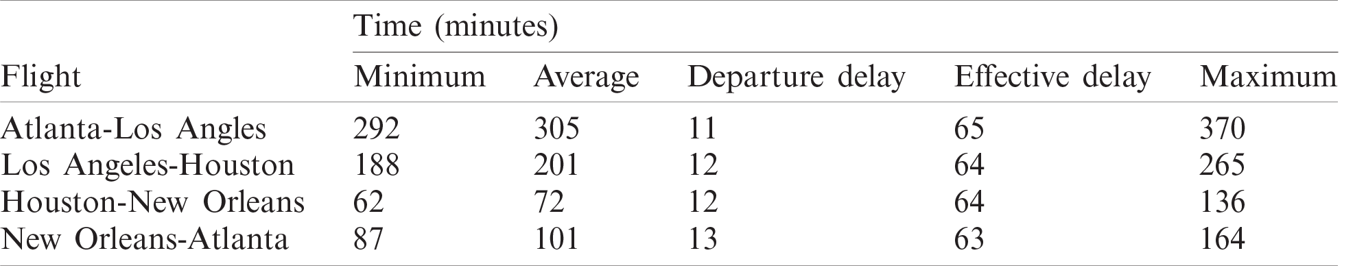
A part of the recorded delays happened in the departure airport before the airplane start moving, this part of time will not consume fuel or the consumption can be neglected, so this time duration can be subtracted from the total delay to cum with the effective delay time. Reference [37] shows a comparison of flight delays across the main US airports. The average flight delays across Atlanta, Los Angeles, Houston and New Orleans airports are estimated to be: 11, 12, 12 and 13 minutes respectively “October 2018 to September 2019”. Tab. 3 demonstrates the flight time data for different flight segments where the minimum flight time is the smaller value of the target and scheduled times, the departure delay is the flight delays across the departure airport, the effective delay is the recorded maximum delay time = 76 minutes the departure delay, the maximum flight time is evaluated by adding this delay to the average flight times.

Table 3: Flight time data for different flight segments

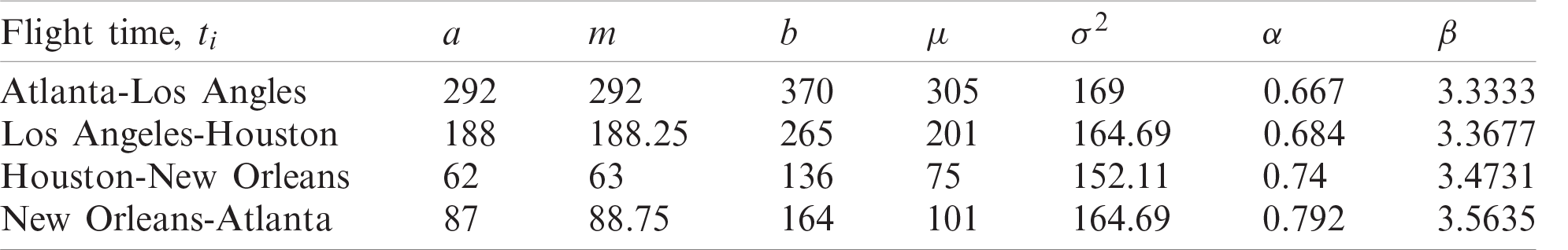
6.2 PERT-Beta Distribution Parameters

Since the target and scheduled flight times are based on somewhat ideal conditions, the optimistic time estimate (a) is equal to the smallest of those times. The expected mean time (μ) is the average flight time. The pessimistic time estimate (b) is calculated by adding the estimate of worst effective flight delay to the average flight time. Knowing (a), (b) and (μ), the most likely time estimate (m) is calculated using Eq. (18) and the variance (σ2) is calculated using Eq. (19). The remaining PERT-beta distribution parameters σ, α and β are calculated using Eqs. (20–21). Tab. 4 shows the distribution parameters of all the flight segments.

Table 4: PERT-beta distribution parameters

Reference [28] expresses the Beta Probability Density Function (PDF) for all the four flight times and one example for the Cumulative Density Function (CDF), Atlanta-Los Angles as shown in Fig. 7. The PDF for all the five probabilistic traveling times are highly right skewed as (m) are very close to (b) than they are to (a) and have the reversed J-shape Beta (α< 1 and β>1). Reference [32] shows that several add-ins such as @Risk (from Palisade Corporation), the Analysis ToolPak add-in in Excel, and Crystal Ball (from Decisioneering) can facilitate the simulation process in the spreadsheet.

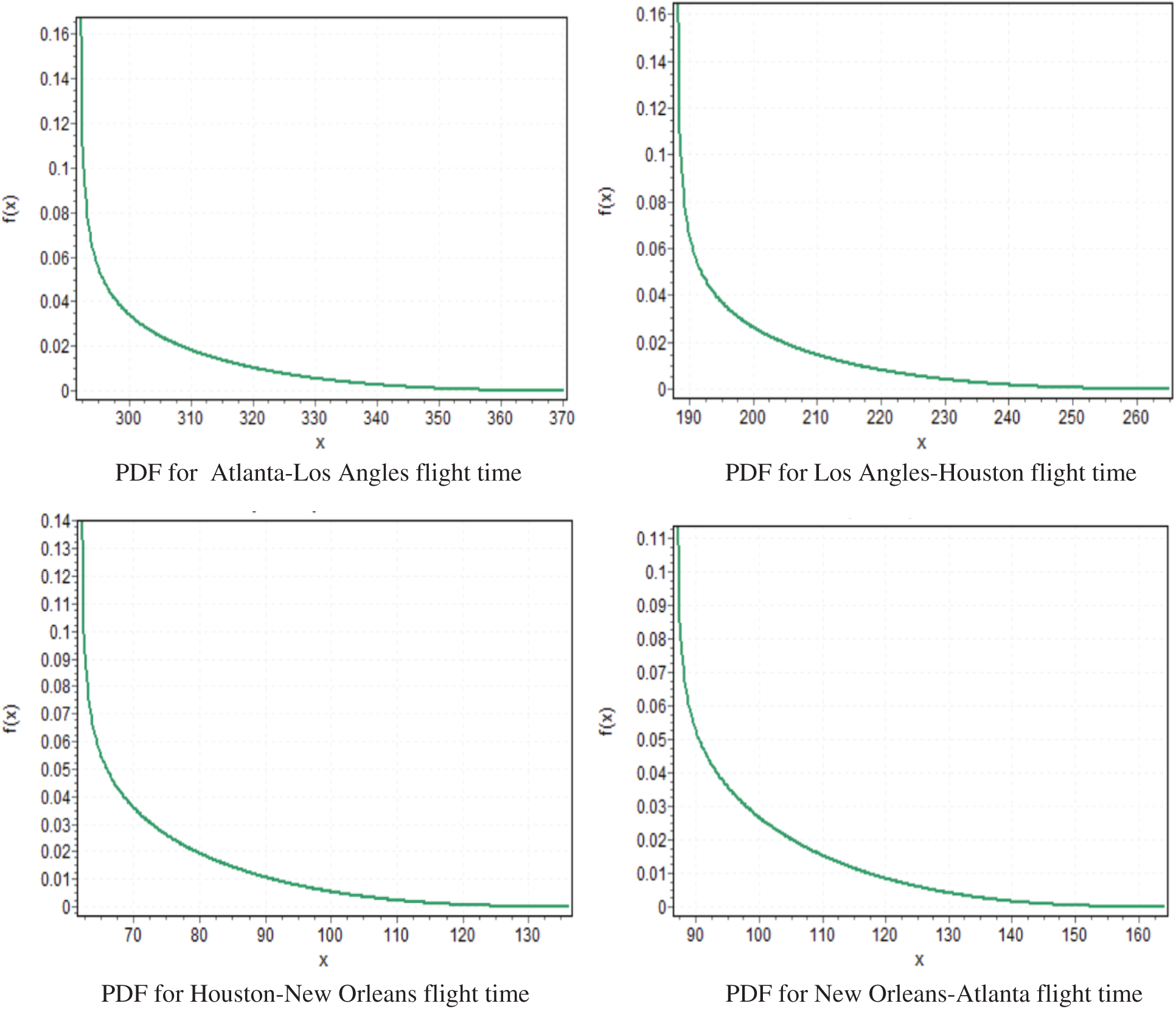
Figure 7: Shape of the BDF for the flight times

7  Solution Procedure

Reference [38] shows that metaheuristic algorithms are widely used in solving different real-world optimization problems. There are various metaheuristic algorithms available in the literature, among them, gaining sharing knowledge based (GSK) algorithm is recently developed and it has been proposed over continuous space. It is based on the concept of acquiring and sharing the knowledge during the human life period. It depends on the two important stages i.e. junior gaining and sharing stage and senior gaining and sharing stage. The working mechanism of the GSK algorithm is explained in detailed way as follows:

Step 1: Let xt(t=1,2…,NP) be the number of persons of a population and each person having D number of fields of knowledge. Each xtp(t=1,2…,NP,p=1,2,…Dim) is represented as xtp=(xt1,xt2,…,xt,Dim). fi be the corresponding objective function values. Firstly, the initial population (xtp0) is randomly generated by the following equation: xtp0=αp+randp(βp-αp).

Where, αp,βp are the lower and upper limits of the decision variables respectively and randj generate a random number in the range 0 and 1.

Step 2: To come up with the two stages, the persons from early middle age acquire knowledge from their known persons. While, the people from middle later stage gain the information with their friends, colleagues and share with other persons with whom they can enhance their knowledge. Therefore, the dimensions of each stages must be calculated using this formula:Dimjunior=Dim×(Genmax-GGenmax)kDimsenior=Dim-Dimjunior where, Dimjunior and Dimsenior represent the dimensions of junior and senior stages respectively, k(> 0) denotes the learning rate, that monitors the experience rate. Genmax is the maximum count of generations, and G is the count of generation.

Step 3: Junior gaining and sharing stage: In this stage, the early aged people gain knowledge from their small networks and share their views with the other people who may or may not belong to their group. Thus, individuals are updated through as:

According to the objective function values, the individuals are arranged in ascending order. For every xt(t=1,2,…,NP), select the nearest best (xt −1) and worst (xt+1) to gain knowledge, also choose randomly (xr) to share knowledge. Therefore, to update the individuals, the pseudo-code is presented in Fig. 8. Where: kf(> 0) is the knowledge factor.

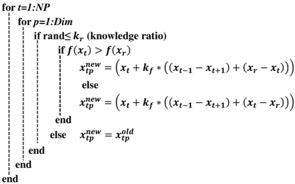
Figure 8: Pseudo-code for Junior gaining sharing knowledge stage

Step 4: Senior gaining sharing knowledge stage: This stage comprises the impact and effect of other people (good or bad) on the individual. The updated individual can be determined as follows:

The individuals are classified into three categories (best, middle and worst) after sorting individuals into ascending order (based on the objective function values).

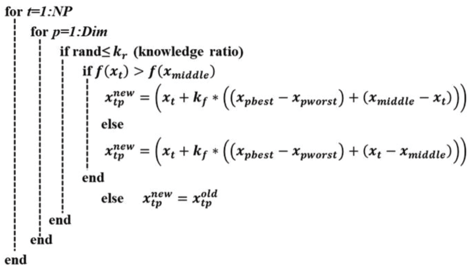
Figure 9: Pseudo-code of Senior gaining sharing knowledge stage

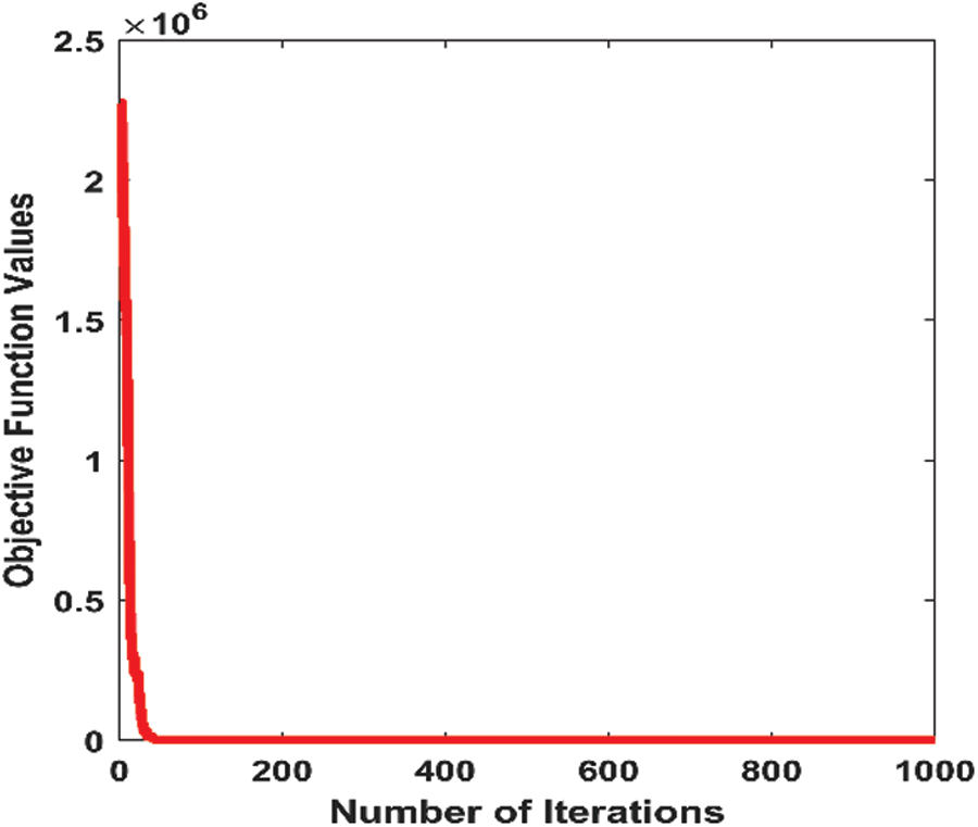
Figure 10: Convergence graph of the optimal solution

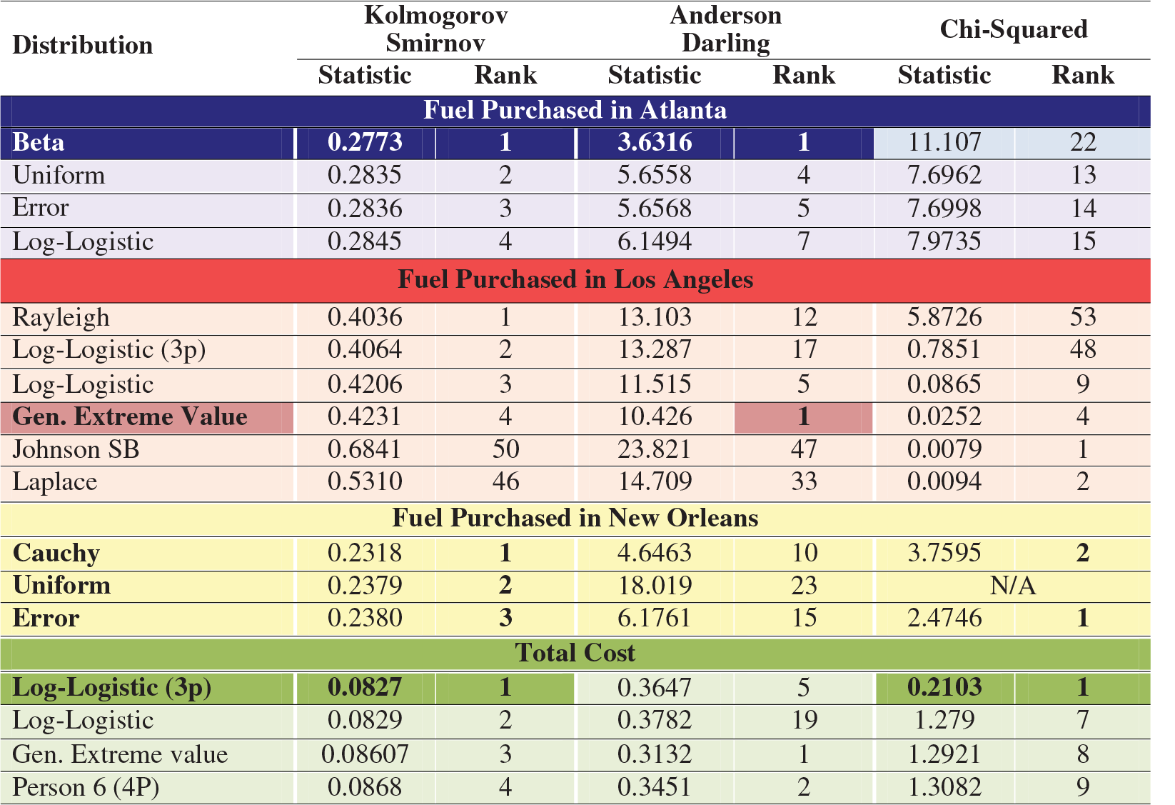
Table 5: Goodness of fit results for the purchased quantities and the total cost

Best individual=100p% (xbest), middle individual=Dim-2*100p% (xmiddle), worst individual = 100p% (xworst)

For every individual xt, choose the top and bottom 100p% individuals for gaining part and the third one (middle individual) is chosen for the sharing part. Therefore, the new individual is updated through the following pseudo-code dictated in Fig. 9, where: p∈[0,1] is the percentage of best and worst classes.

Fifty simulation runs are performed and the 4 random flight times according to the BERT-beta distribution are used in the described model, the optimum solutions are recorded for further evaluation. The convergence graph of one optimal solution is shown in the Fig. 10.

The optimum solutions including purchased fuel quantities and total cost are recorded, from the data, it is shown that the amounts of purchased fuel in airports Atlanta, Los Angeles and New Orleans are very sensitive to variations in the flight time durations, while the purchased fuel amount in Houston airport = 0 for all simulation runs. Tab. 5 presents the goodness of fit summary of the purchased quantities and total cost and Fig. 11 represents the BDF for Atlanta, Los Angeles, New Orleans and cost.

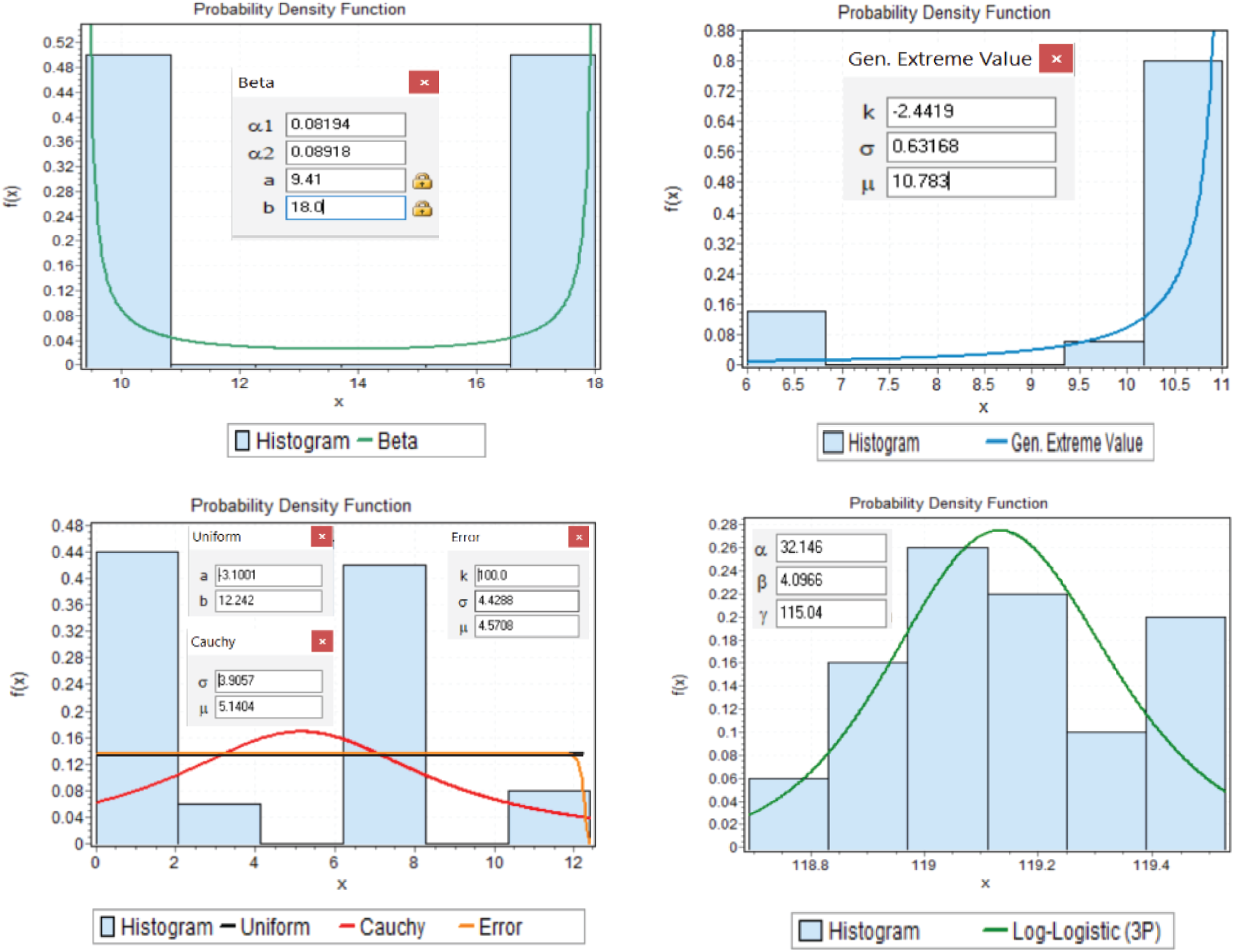
Figure 11: BDF for Atlanta, Los Angeles, New Orleans and cost

8  Conclusions and Points for Future Researches

The main conclusions for this paper can be summarized as follows:

1.    The aircraft refuelling task for a stochastic flight with a ferrying strategy and discounted fuel prices is addressed through a mixed binary nonlinear mathematical programming model. The proposed mathematical model specifies the best refuelling strategy so that to minimize the total refuelling costs.

2.    Handling the case of discounted fuel prices is done by two methods: adding binary dummy variables and curve fitting methods. A comparison of the two methods is illustrated.

3.    The stochastic characteristics appears when addressing the flight times in real-life problems. The simulation process is utilized to generate random values according to PERT-beta distribution and then the simulation output is collected to produce the needed results.

4.    An application case study for a domestic U.S. airline flight rotation problem with complete problem definition, stochastic mathematical model formulation and the simulation run procedure are presented. The produced 50 simulation runs are solved, the output histograms and distributions for the purchased amounts of jet fuel and for the total cost are obtained.

5.    The obtained results suggest that the introduced probabilistic model is sensitive to fluctuations in flight times which are considered as random variables with BERT-beta distribution. While the stochastic nature of the problem has a great influence on the amounts of fuel purchase strategy, it is not so significant on the total cost of the flight route.

6.    The proposed mathematical model is so general that it is applicable for any other national or international airline flight rotate problem with available real data.

7.    The stochastic nature of the problem has a great effect on the amounts of purchased fuel from airports. On the other hand, its effect is not significant on total flight cost.

8.    The GSK algorithm is able to find the solution of the mathematical model and proves its robustness and convergence capability to obtain the solution.

The main points for future researches can be stated in the following points:

1.    To consider other parameters affecting the amount of fuel burned.

2.    To apply the same mathematical model for other national and international airlines.

3.    To evaluate significant environmental impacts of fuel tinkering due to excess fuel burnt and its negative environmental impacts.

4.    To apply similar problem formulation to maritime transportation sector.

5.    Evaluate the performance of the GSK procedure in dealing with different types of complex mathematical programming problems, and to investigate more extensions of GSK.

Acknowledgement: The authors extend their appreciation to the Deanship of Scientific Research at King Saud University for funding this work through research group number RG-1436-040.

Funding Statement:The research is funded by Deanship of Scientific Research at King Saud University research group number RG-1436-040.

Conflicts of Interest: The authors declare that they have no conflicts of interest to report regarding the present study.

This work is licensed under a Creative Commons Attribution 4.0 International License, which permits unrestricted use, distribution, and reproduction in any medium, provided the original work is properly cited.