DOI:10.32604/cmc.2021.016534
| Computers, Materials & Continua DOI:10.32604/cmc.2021.016534 | |
| Article |
An Attention Based Neural Architecture for Arrhythmia Detection and Classification from ECG Signals
1Department of IT, VNR Vignana Jyothi Institute of Engineering & Technology, Hyderabad, 500090, India
2Department of CSE, JNTUH, Hyderabad, 500085, India
3Department of CSE, Vaagdevi College of Engineering, Warangal, 506005, India
4Kakatiya Institute of Technology and Science, Warangal, 506015, India
*Corresponding Author: Nimmala Mangathayaru. Email: mangathayaru_n@vnrvjiet.in
Received: 04 January 2021; Accepted: 11 April 2021
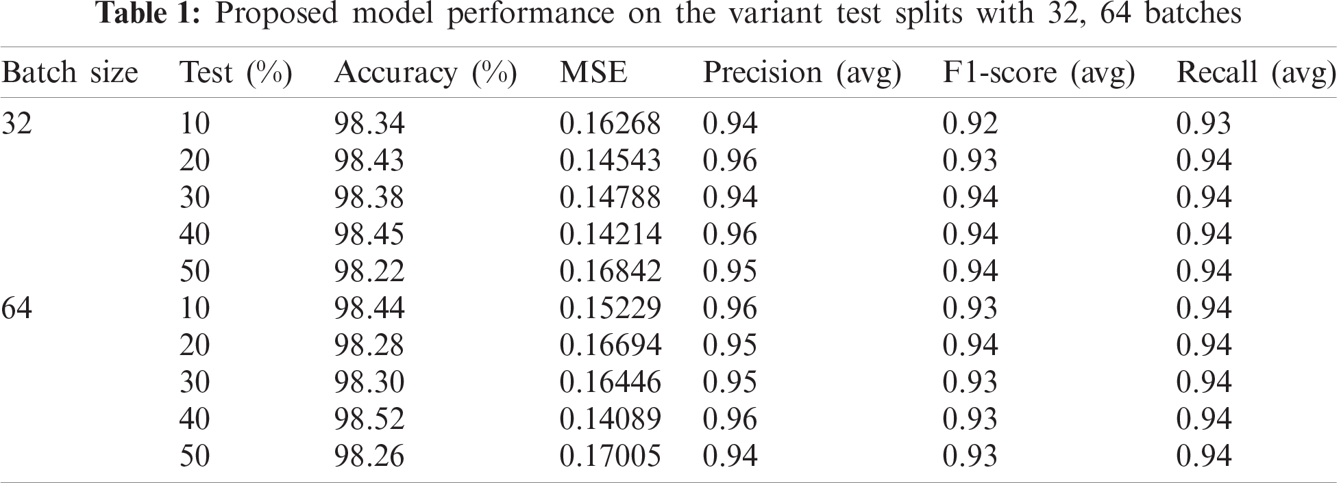
Abstract: Arrhythmia is ubiquitous worldwide and cardiologists tend to provide solutions from the recent advancements in medicine. Detecting arrhythmia from ECG signals is considered a standard approach and hence, automating this process would aid the diagnosis by providing fast, cost-efficient, and accurate solutions at scale. This is executed by extracting the definite properties from the individual patterns collected from Electrocardiography (ECG) signals causing arrhythmia. In this era of applied intelligence, automated detection and diagnostic solutions are widely used for their spontaneous and robust solutions. In this research, our contributions are two-fold. Firstly, the Dual-Tree Complex Wavelet Transform (DT-CWT) method is implied to overhaul shift-invariance and aids signal reconstruction to extract significant features. Next, A neural attention mechanism is implied to capture temporal patterns from the extracted features of the ECG signal to discriminate distinct classes of arrhythmia and is trained end-to-end with the finest parameters. To ensure that the model’s generalizability, a set of five train-test variants are implied. The proposed model attains the highest accuracy of 98.5% for classifying 8 variants of arrhythmia on the MIT-BIH dataset. To test the resilience of the model, the unseen (test) samples are increased by 5x and the deviation in accuracy score and MSE was 0.12% and 0.1% respectively. Further, to assess the diagnostic model performance, AUC-ROC curves are plotted. At every test level, the proposed model is capable of generalizing new samples and leverages the advantage to develop a real-world application. As a note, this research is the first attempt to provide neural attention in arrhythmia classification using MIT-BIH ECG signals data with state-of-the-art performance.
Keywords: Arrhythmia classification; arrhythmia detection; MIT-BIH dataset; dual-tree complex wave transform; ECG classification; neural attention; neural networks; deep learning
Arrhythmia is ubiquitous worldwide and there is still a major population at risk. The ECG signals are highly efficient and used as a gold-standard to detect the presence of arrhythmia and critical conditions such as cardiac arrest. So, detecting arrhythmia using ECG signals is challenging for researchers. In this era of automation, deep learning has made strides in various fields such as computer vision, language processing, and signal processing in developing state-of-the-art models on large scale databases. Further, deep learning has advanced in bio-medical imaging and bio-medical signal processing. Hence, it is aimed to develop a diagnostic model by extracting features from ECG using DT-CWT and processing them with help of the proposed neural architecture.
It is observed that the signals recorded by ECG are a combination of PQRS waves and these waves detect the heart functionality by identifying various characteristics. Certain features are extracted from the signal by pre-processing it with various transformation techniques in which continuous wavelet transform and discrete wavelet transform are frequently used. Sequentially these extracted features are then processed using various learning algorithms such as k-nearest neighbors (k-NN), Support vector machines (SVM), Multi-layer-perceptron (MLP), Singular value decomposition (SVD), etc. The pre-processing techniques are implied for extracting the features from ECG signal widely used Discrete wavelet transformation (DWT), which is sensitive to shift-invariance and downgrades the quality of the signal while reconstructing the decomposed signal. In the subsequent processing step, most of the methods include generic machine learning algorithms (classification or clustering algorithms) or an MLP which does not capture temporal invariances and eventually harms the performance by reducing the generalization. Hence the two key steps to provide a diagnostic model are, (a) an appropriate pre-processing of the signal (DT-CWT) (b) a processing step to prognosticate the disease (neural attention). To overcome the drawbacks of the existing research, the proposed diagnostic framework implies DT-CWT and neural attention mechanism to provide a significant solution.
The impact of MIT-BIH data was shown by George et al. [1], which acted as a catalyst and gave rise to numerous works that provide insights on automated devices to diagnose arrhythmia. Markos et al. [2] used time-domain analysis to extricate features and then arranged them in distinct combinations, which are utilized as input for neural networks. Sixty-three different types of neural networks were formed. The output of these networks was deployed to a decision tree to diagnose arrhythmia. Karimifard [3] worked on modelling of signals, who later used a Hermitian basis function to get a feature vector and sent to a k-nearest neighbor classifier to classify seven types of arrhythmia, which [1–4] obtained sensitivity and specificity of 99.0% and 99.84% respectively. He also concluded that the size of the feature vector affected the training time of the model. Mohammadzadeh et al. [4] took features from the signal by linear and non-linear methods, which were reduced by Gaussian discriminant analysis (GDA) and used an SVM to recognize six classes of arrhythmia with a sensitivity of 95.7% and specificity of 99.40%. Chi et al. [5] focused on quick prediction of the disease by pulling out PQRST features from the ECG signal and later used Linear Discriminant Analysis for grouping five different classes of arrhythmia and achieved an accuracy of 96.23%.
A unique use of the kernel Adatron algorithm was combined with SVM by Majid et al. [6]. He explained the drawbacks of a multi-layered-perceptron (MLP) and differentiated the training and testing time of these two methods. Hamid et al. [7] performed Complex wavelet transformation (CWT), Discrete wavelet transformation (DWT), Discrete cosine transformation (DCT) feature extraction methods separately on the signal and formed four different structures using MLP, then the other four using SVM and deduced the efficient use of a feature extraction method by the training time of the model [5–10]. Oscar [8] preprocessed the signals by QRS extraction method and used fuzzy KNN, MLP with backpropagation, and MLP with scaled conjugate gradient backpropagation (GBP) to get the output matrix. Later these three matrices were combined and sent to the fuzzy inference system to get the result. This achieved an accuracy of 98%. Roland et al. [9] presented an artificial neural network that took signals that are preprocessed by Fast Fourier Transformation (FFT) as an input and then categorized five classes of arrhythmia.
The importance of PQRST wave properties was also discussed here. Yeh et al. [10] proposed a novel preprocessing method along with Cluster analysis (CA) to classify 5 distinct classes and attained a total classification accuracy (TCA) of 94.30%. Stefan [11] developed an android application for real-time detection of arrhythmia by Decision Trees (DT). This model clocked a sensitivity of 89.5% and specificity of 80.6%. Elgendi [12] introduced the application of the moving averages method on ECG signals for detection of P and T waves by addressing four sources of noise which altered the quality of the signal and obtained a sensitivity of 98.05% and specificity of 98.86%. Manu et al. [13] extracted features using DTCWT and merged another four features (AC power, Kurtosis, Skewness, and timing information). This feature set was passed into an MLP and got an accuracy of 94.64% and a sensitivity of 94.6%. Ahmet et al. [14] showed a comparison between the performance of bagged decision trees and a single decision tree with the input of nine features which was taken from ECG signal by applying Low Pass Filter, High Pass Filter, form factor (FF) computing, FF ratio to previous one (FFR), RR ration to the previous RR ration (RRR), RR difference from mean RR value (RRM), skewness, linear predictive coding (LPC) and the cumulated ensemble method outperformed a single decision tree with an accuracy of 99.15%. Mehrdad [15] improved the signal quality by un-decimated wavelet transformation (UWT) and then proposed a method that combined Negatively Correlated Learning (NCL) and Mixture of Experts (ME) which is known to provide an excellent recognition rate. The model is used to group premature ventricular contraction (PVC) arrhythmia and Normal heartbeat classes and achieved accuracy, sensitivity, the specificity of 96.02%, 92.27%, and 93.72% respectively. Ping [16] proposed an adaptive feature extraction method based on wavelet transformation and a modified voting mechanism consists of K-means clustering, one against one SVM to enhance the recognition rate and got an accuracy of 89.2%. Joachim [17] worked on the categorization of poor and good signals. An alarm is set off when the parameters are not within a given scale. QRS extraction method along with SVM was used to reach this objective. Patricia [18] presented a Learning Vector Quantization (LVQ) algorithm with SVM to classify arrhythmia. However, the comparisons were made with simulated data. A total of 15 classes were grouped with three different architectures and the best architecture got an accuracy of 99.16%. Ali et al. [19] performed a diagnosis of arrhythmia with the help of Alex net and prior QRS detection was done. The signal was converted to a 256 × 256 sized image and then passed into the network. The recognition rate and accuracy are 98.5% and 92%. Joy [20] implemented DCT transformation of waves and used Probabilistic Neural Network (PNN) for efficient detection of disease [11]. Vasileios [21] showed false beat detection effectively by detecting QRS peaks then filtering false beats using SVM and concluded that QRS peaks are very important for the detection. Rashid et al. [22] proposed a new method that showed promising results by using Gaussian mixture modeling (GMM) with expectation maximization (EM), Combined with statistical and morphological features. Accuracy for class-oriented is 99.6% and for subject-oriented is 96.15%. Serkan et al. [23] also made an android application using 1-D convolution to classify supraventricular ectopic beat (SVEB) and ventricular ectopic beat (VEB). FFT with DCT was used in feature extraction and obtained an accuracy of 99.0%, 97.2% for each class.
From the previous research works, it is observed that (pre-processing part) many methods do not capture temporal relationship among the data. If they capture temporal dependencies, they do not persist with long term dependencies. So, if long term dependencies are provided there are no sequential patterns, which provide attention to the network determining the importance factor. So, these loops are overhauled with the use of attention embedded neural architecture by capturing long term temporal dependencies. Further, some loops are addressed in the pre-processing section and they are overridden by utilising DT-CWT and are mentioned in the successive section.
In this research, the contributions to the body of the knowledge are mentioned as,
• Dual-Tree Complex Wavelet Transform (DT-CWT) method is implied to overhaul shift-invariance and aids the signal reconstruction to extract significant features. Further, a small set of features are extracted using the Pan-Tomkins algorithm and are adjoined with the features extracted from DT-CWT.
• A neural attention mechanism is implied to capture temporal patterns from the extracted features of the ECG signal and to discriminate distinct classes of arrhythmia. The proposed attention model is end-to-end trained by carefully optimizing the hyperparameters.
As mentioned, the two important steps are involved to complete the proposed automated system. This section aims to give a clear understanding of mathematics related to these two steps and explains the unique capabilities.
In this paper, ECG recordings acquired by the arrhythmia laboratory of Boston’s Beth Israel Hospital are used and this database is known as the MIT-BIH arrhythmia database. ECG recordings are collected using Del Mar Avionics model 445 two-channel reel to reel Holter recorders. These signals were filtered using bandpass filters with frequency in the range of 0.1–100 HZ and are digitized by Del Mar Avionics 660 playback unit with a sampling rate of 360 samples per second. This database consists of forty-eight half-hour excerpts of two-channel twenty-four-hour, ECG recordings from 47 subjects as record number 201. The first twenty-three records are drawn from a collection of four thousand Holter tapes and the other records include uncommon heartbeat irregularities but have great clinical significance. The subjects include twenty-five men and twenty-two women who are aged between twenty-three to eighty-nine.
The most frequently used ECG leads in this database are modified limb lead 2 (MLII) for channel one and v1 for the other channel. V2, V4 and V5 are also used occasionally, based on the subjects. Fusion Ventricular (FV), VEB, right bundle branch block (RBB), paced beat (PB), Normal (N), ventricular contraction (VC), left bundle branch block (LBB), atrial premature beat (APB) are the different classes of arrhythmia that are used in the task of classification to evaluate the model.
4.2 Feature Extraction (Pre-Processing)
As an insight, pre-processing step is important to capture appropriate features which in turn obliges prognosticate arrhythmia. After extensive research on what would be the best practice to get the features based on prior knowledge, it is to be deduced that wavelet transformation for the first step is the best practice for MIT-BIH arrhythmia. The QRS complex signal is pulled with a sample of 256 of which 128 samples are considered from the left side of the R peak and 128 samples from the right. Later wavelet transformation is applied to get a set of required features. As a note, the database reflects certain noise in the signal and the cause of it are described below,
• The frequency from the power supply usually manipulates the signal, this is known as the powerline interface.
• Our muscles often tend to contract and expand, which regularly gets combined with cardiac muscles and end up giving a signal with noise
• A signal quality often depends on the contact between the lead and skin, there are some times that a movement by the patient corrupts the signal and this is described as motion artefact.
The above-discussed problems are solved by implementing the Pan-Tomkins and including it as one of the important features for signal pre-processing. These findings are addressed in discovering the QRS complex by Pan–Tomkins [24]. A signal undergoes four steps in this algorithm. Initially, to attenuate noise, the signal is passed to a bandpass filter, which eliminates motion artefact and makes the signal more stable. A differentiator is used to get the slope of the signal and solve the baseline drift problem. This is followed by a squaring function that helps to remove get absolute value and limit false positives generated by T waves. Finally, moving-window integration is used to smooth the curve and get information about the slope of the signal. The steps are implemented for a signal (considered from the database) and are visually illustrated in Fig. 1. Wavelet transformation is applied to the extracted QRS complex signal where a wavelet acts as a window function. All the wavelet transformations are in the compressed or shifted form of the mother wavelet and the different versions of the mother wavelet are described in Eqs. (1)–(3). In Eq. (1) [25], S is the inverse of the frequency of the signal, which can be used to get low and high-frequency signals and to make the wave thinner or broader. T is used to translate wavelet across the signal. Wavelet transformation helps in analysing the different frequencies at different locations; This is known as multi-resolution analysis. By changing the values of S, the wavelet can be obtained in expanded or in compressed form, which is known as scaling. For non-stationary waves, CWT is used, however, the upper limit and lower limit of CWT tends to infinity. This means that there would be a huge number of coefficients that are to be calculated at every possible position. (in Eq. (2)) [26].
where,
To reduce the number of coefficients, DWT is used instead of CWT (Eq. (3)) [27]. This is achieved by choosing a, b in powers of two and so, the DWT is calculated (computationally) by multilevel decomposition. The signal is further passed into a low pass and high pass filter and the two filters utilized are orthonormal by construction. Initially, the signal is passed to a low pass filter to get approximate coefficients and then again to a high pass filter to get detailed coefficients and are downsampled by 2 successively. The approximate coefficients are iteratively processed in the same way to get low pass portions as well as high pass portions. Fig. 2 visually explains the complete overview of the DWT decomposition process.
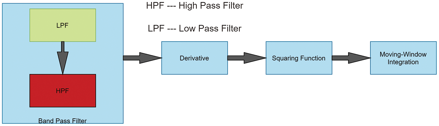
Figure 1: Steps in Pan–Tomkins algorithm
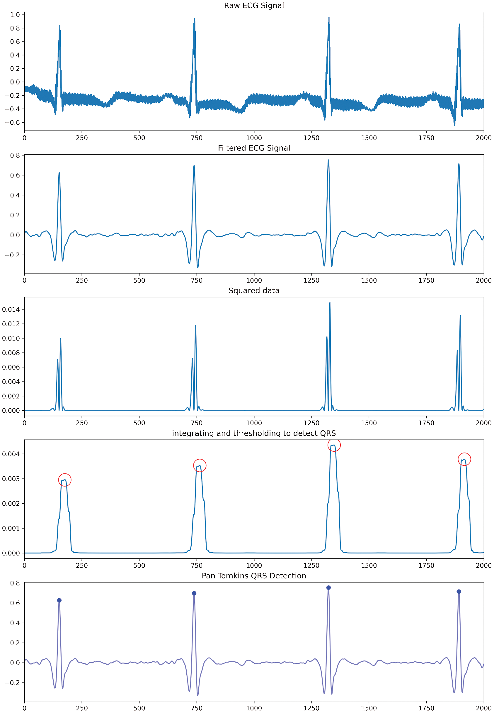
Figure 2: Transformation of the signal after every individual step using pan Tomkins algorithm
Yet after decomposition, it still lacks Perfect Reconstruction (PR) and does not provide a shift in-variance. To overcome this, Dual-Tree Complex Wave Transformation (DT-CWT) is used [28]. DTCWT employs a complex-valued scaling function and wavelet. The Eqs. (4) and (5) show the functions used in DT-CWT, where
In Fig. 4, Tree(A) is used to acquire the real part coefficients and Tree (B) is utilized to get the imaginary part coefficients. The low pass filter is slowed down by one-fourth of the sample for non-symmetry, which helps in achieving the PR of the signal. The filters used in both the trees are orthonormal to each other and the reverse of decomposition provides the synthesis of the signal. Next, fourth and fifth level detailed coefficients are taken from both the trees. Then 1-D FFT is applied with the obtained features from these levels and another four features are appended to this feature set. The four features are AC power, kurtosis, skewness and timing information and cumulated twenty-eight features from DT-CWT are extracted from this process and are ready to be fed into the classifier.
4.3 Classification (Processing)
In the past few years, Feed Forward Neural Networks (FNN’s) dominated the automation field. Even after their efficient performance throughout the years, they are still short of remembering long term dependencies and do not work well with the time-series data. Recurrent Neural Network’s (RNN’s) are used to overcome this drawback. The central theme of the architecture proposed in this section is based on Recurrent Neural Networks and before explaining the proposed architecture, a detailed summary of the Recurrent Neural Networks and their variants are explained below.
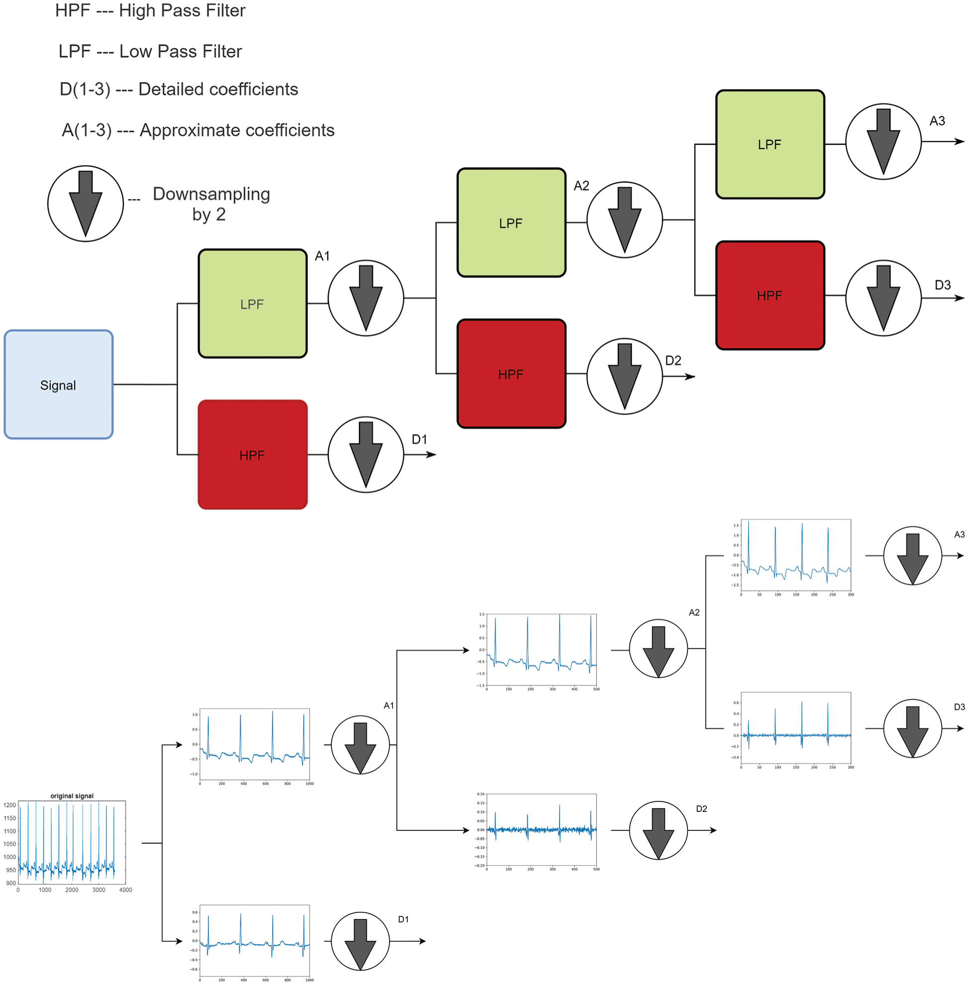
Figure 3: DWT architecture and transformation of a signal at every level of decomposition
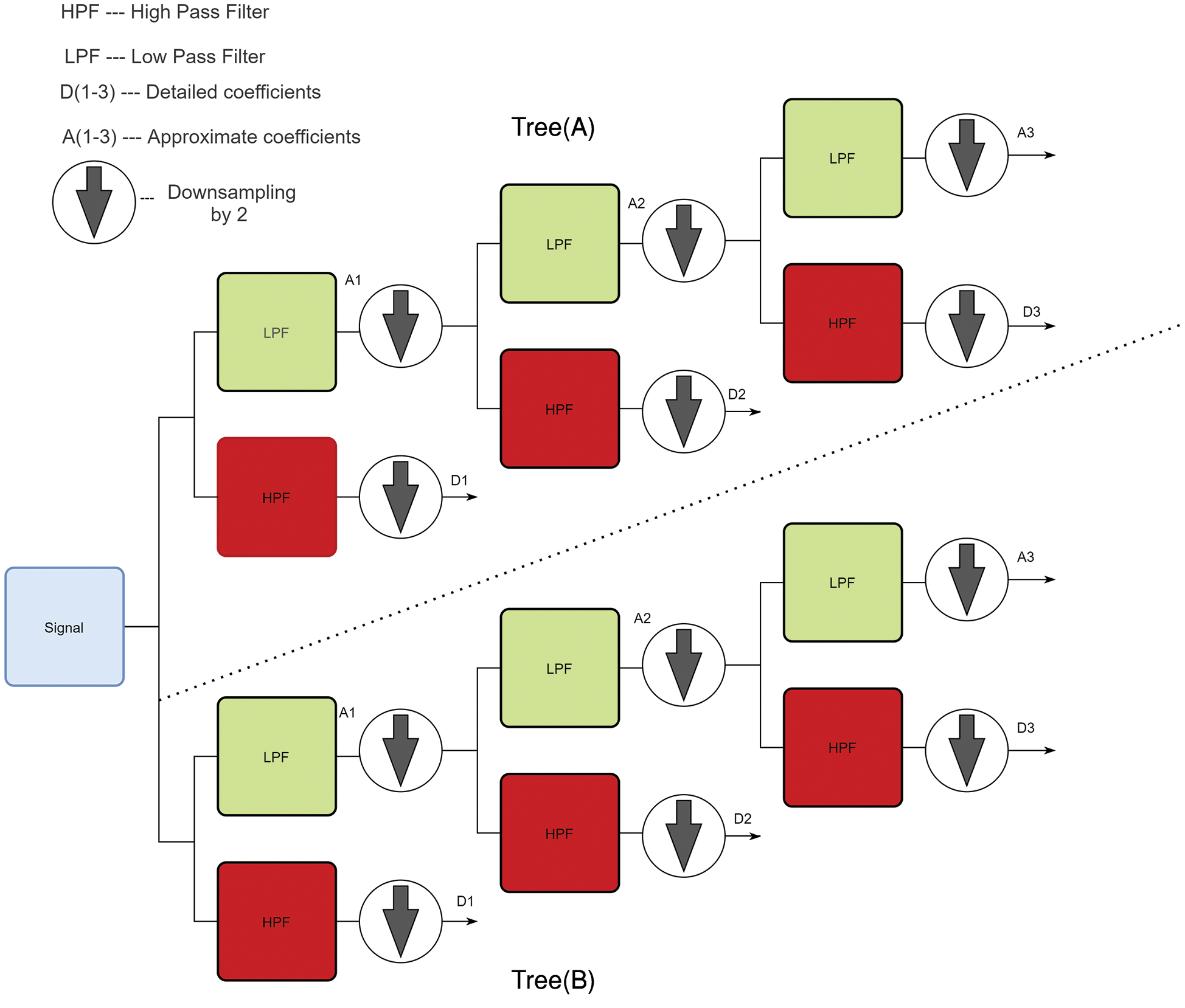
Figure 4: Architecture of DT-CWT
4.3.1 Recurrent Neural Networks (RNN)
Unlike FNN’s, RNN’s can consider the input of different lengths and provide an output of different lengths. This feature has increased the scope of applications of Deep Learning, such as image captioning and language translation. RNN’s have a loop to their unit which helps to store information. These networks play on a recursive function that helps to generate a new state at the time (t) by the information of its old state at the time (t − 1). Eq. (6) [29] shows the recursive function which is a tanh function that has weights and linear operations in it.
These networks use backpropagation through time to calculate the gradient. As the number of units in the network increases, the gradient value would come close to zero, because of this the weights would not add any information to the network and this problem is known as the vanishing gradients.
4.3.2 Long Short-Term Memory (LSTM)
Long Short-Term Memory (LSTM) is a different type of cell used in recurrent neural networks which were found by Sepp et al. [30]. In an LSTM cell, there are various gates, where each gate has its purpose. Lines that are connected to the gates carry a vector that is used to perform a linear operation and provide the output as required. These gates have full control over the information that has to be retained or removed. The gates in LSTM have sigmoid and pointwise operations and the information is initially passed through the LSTM network by the cell state. Only with the cell state, different operations can be performed from the information provided by the cell state to understand LSTM clearly. The working of an LSTM cell is divided into four steps.
Step 1: To know what information should be forgotten from the previous state. This is done by the ‘forget gate also known as the first layer of LSTM. It takes
Step 2: To take the required information which is done by the input gate that tells what to write to cell state. Two functions act in this gate.
Step 3: First is the sigmoid layer known as the input gate layer
Step 4: A tanh function is used which produces a candidate set
Eqs. (12) and (13) are used to update the cell state; first, Eq. (10) is multiplied by
After updating the cell state the output of the LSTM cell is calculated, this is calculated after the input passes through a sigmoid layer and then through a tanh function of
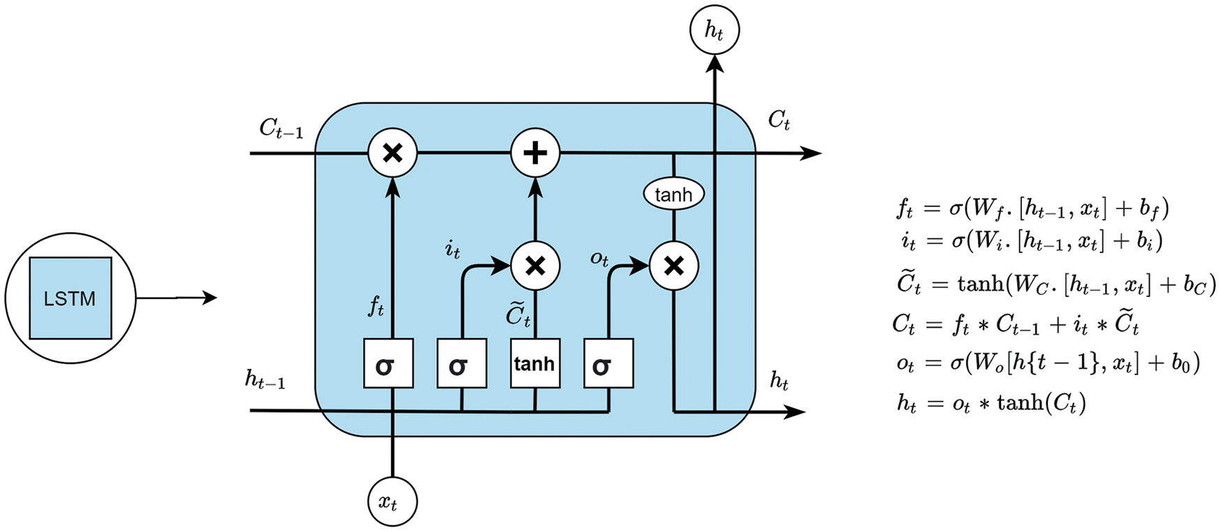
Figure 5: An LSTM unit
4.3.3 Gated Recurrent Units (GRU)
The gated recurrent unit (GRU) [32] is another variant of the Recurrent Neural Network and is similar to the LSTM with some changes. Due to the changes which are made, GRU tends to work faster than the LSTM network and gives an advantage over it and this can also be explained in 4 steps that are below:
Update Gate: The functionality of the update gate is to decide what information is to be taken from the previous cell. It takes
Reset Gate: Reset gate works the same as the forget gate in LSTM.
Current information: By using the reset gate,
Output: update gate is employed to get the final output
4.3.4 Bi-Directional Units (Bi-LSTM and Bi-GRU)
It is seen that bi-directional RNN leverages performance compared to that of unidirectional RNN on speech data. Firstly, the state neurons are divided into two different time directions which are considered as forward and reverse states and the output from the reverse state is not connected to the input of forwarding states, and vice versa. With the assistance of these two sequential time directions, the input data assess the future and past dependencies. This helps to understand long-term dependencies. While training bi-directional RNN’s the weighs are updated not only via forwarding pass but also through backward pass [34]. Additionally, it is observed that bi-directional LSTM units outperform in phenome classification and recognition tasks with fewer computations i.e., epochs [35]. Similarly, Bi-directional GRU’s can draw desirable outcomes similar to that of bi-directional LSTM’s [36]. Hence, it is aimed to connect sequential bi-directional LSTM and GRU units cautiously for outperforming the classification of ECG signals by acquiring their temporal patterns as shown in Fig. 6.
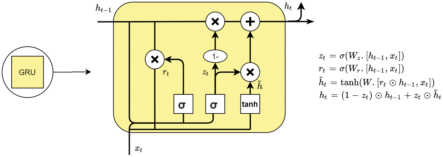
Figure 6: A single gated recurrent unit (GRU)
4.3.5 Proposed Neural Architecture
The attention mechanism in neural networks was first implied by Dzmitry et al. [37] to memorize long sequences in decoder architecture. A neural architecture is proposed with an embedded attention mechanism for the classification of 8 distinct kinds of arrhythmia from ECG signals. The pre-processed signal from DT-CWT is fed into the proposed neural architecture. The input is merged into two sequential stacked layers with two variant patterns. At first pattern, bi-directional LSTM units are sequentially arranged with respective layer normalization and dropout layers [38,39]. In the second pattern, bi-directional GRU units are stacked similar to that of the previous pattern. Then, the output sequence from pattern-i is multiplied with pattern-ii to imply attention.
For a definite time step ‘t’, both the bi-directional LSTM and GRU sequence units attempt to perform attention by a scalar product as mentioned in Eq. (19). This attention mechanism is proposed as global attention to extracting invariant temporal patterns [40].
Then the resultant multiplied output sequence proceeds as input to a GRU layer and next fed into a fully connected feed-forward network. The complete model architecture and its related parameters are depicted in Fig. 7. The fully connected network consists of 128 unity in the first layer with ReLU as activation and the final layer consists of 8 neurons which are activated with softmax. The complete model consumed 106K trainable weights and negligible non-trainable weights consumed with the usage of layer normalization layers. The model was trained on 5 variant test patters.
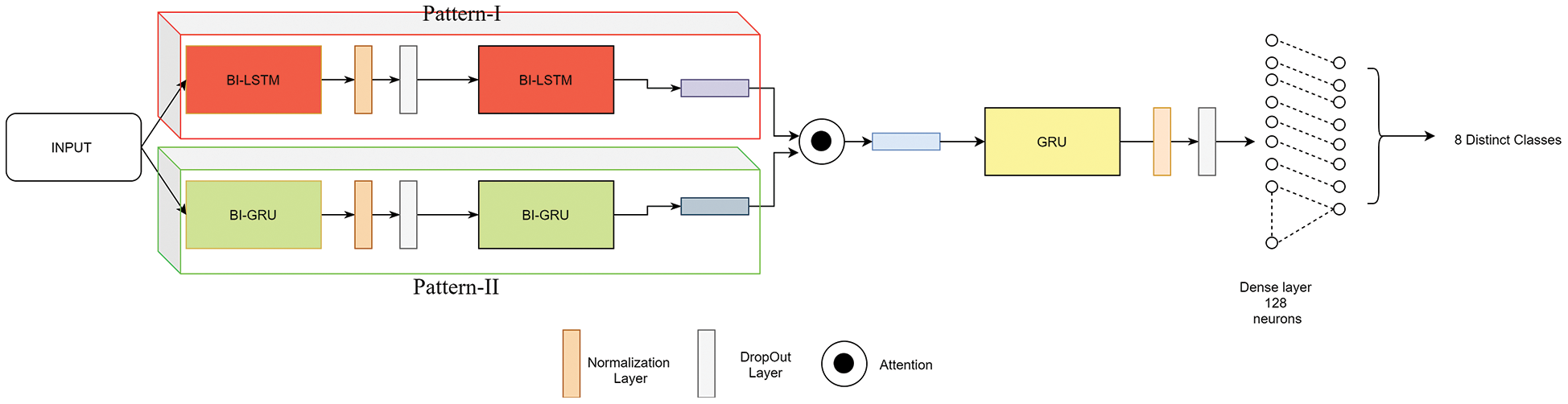
Figure 7: Proposed neural architecture implied with an attention mechanism
As mentioned above, to leverage the model performance, training and testing samples are split into multiple variants ranging from 10% to 50%. The complete analysis is carried out on various standard classification metrics and to study the proposed model behaviour, an accuracy score is chosen as the gold standard. Similarly, to study class wise performance precision, f-1 score recall is utilized. MSE is used to assess the predictability of the model which depicts the error attained due to imperfect predictions. Finally, AUC-ROC curves are generated to assess the diagnostic performance of the proposed model [41].
As AUC-ROC curves are sample invariant in nature as they are insensitive to the alterations implied in the class distributions. These curves are plotted class-wise to interpret the performance of the model at each class level. As a note, AUC-ROC visualizations can be obliged as they decouple the performance of the classifier from skewness in classes and error costs presented in Fig. 8. The proposed model is trained with two variant batches of 32 and 64 respectively. All the above-mentioned classification metrics are evaluated for all the test variants with two different batch sets. Large batches are acquired during training neural networks to minimize the generalization gap [42]. Hence, a large set of batches are considered with sizes of 32 and 64. (illustrated in the Tab. 1). In the feature extraction step, the Pan Tomkins method is employed to extract QRS points of the signal which play an important role in determining r-peak which helps to detect heartbeats. A large set of features are drawn out by using DT-CWT. This transformation is shift-invariant and provides PR. Most of the signal transformation methods lack these properties which can cause imperfect prediction and increase the chance of misclassification.
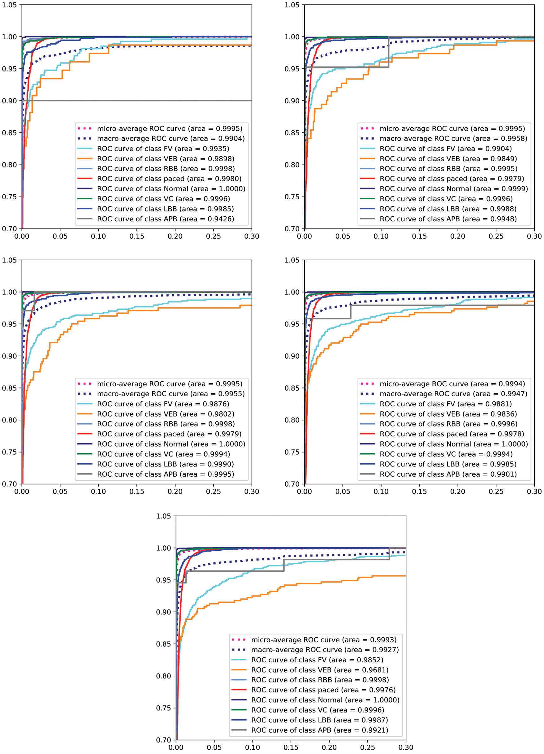
Figure 8: Visualizations of AUC-ROC curves for 64 batch for test size from 10%, 20%, 30%, 40%, 50%

The proposed network used adam [43] as an optimizer with a learning rate of
Generally, RNNs understand the temporal dependencies but they lack understanding in long term dependencies where LSTM overcomes the problems of RNN by understating long-term temporal relationships in the data. But LSTMs are computationally expensive and do have the problem of gradient vanishing with increasing units to a greater extent. Whereas GRU contains fewer gates compared to that of LSTM networks and overcomes the problems of LSTMs. GRUs are computationally faster compared to RNN’s and LSTMs. As most of the research focuses on designing a neural architecture utilizing these units with changing the number of time steps, units and stacking pattern. To leverage predictive capability neural attention is implied by undersetting the temporal pattern extracted from the signal. So, by providing neural attention, the minute redundancies and noise captured during feature extraction can be regulated to a greater extent. This provides greater performance compared to that of remaining neural networks. Various previous work is studied and curated, and our method outperforms the existing literature, and the depicted results are tabulated (illustrated in Tab. 2).
As a note, the research was conducted to study arrhythmia without using signal patterns i.e., carried out by classifying variant attributes involved in predicting cardiovascular diseases [44] and also carried by implying PPG signals [45]. To see the future perspective of the proposed work, it can be figured out traditionally, the current deep learning applications have considered existing distance functions in the research literature for similarity computations but did not try to fit in new functions for similarity computations [46–50]. There is a possibility to devise threshold and similarity functions to suit deep learning applications [51–55]. For instance, recent research contributions propose various similarity and threshold functions for temporal pattern mining which can be redesigned to suit deep learning applications [56–60].
In this research, a novel attention-based neural architecture is built to vanquish the loops of existing methods for classifying ECG signals. It can be stated that the proposed model is sample invariant as it has minute error variation when test samples increased five times. AUC-ROC plots are illustrated to provide a vivid understanding of the performance of the proposed diagnostic model. In a worst-case scenario, the model provides a micro averaged AUC of 0.9904. Even with numerous advantages, it is seen that the proposed model can consume high memory while embedding the model into a real-world application. The training procedure adapted is tested on two batches instead of a dynamic sampling is preferred to improve performance. In future, it is aimed to provide a salient model by acquiring humongous data with less computational capability and higher performance.
Acknowledgement: The authors acknowledge JNTUH/TEQIP-III, for providing research fund (Ref: No. JNTUH/TEQIP-III/CRS/2019/CSE/08).
Funding Statement: This research was partially supported by JNTU Hyderabad, India under Grant proceeding number: JNTUH/TEQIP-III/CRS/2019/CSE/08. The authors are grateful for the support provided by the TEQIP-III team.
Conflicts of Interest: The authors declare that they have no conflicts of interest to report regarding the present study.
1. M. B. George and R. G. Mark, “The impact of the MIT-BIH arrhythmia database,” IEEE Engineering in Medicine and Biology Magazine, vol. 20, no. 3, pp. 45–50, 2001. [Google Scholar]
2. T. G. Markos and D. I. Fotiadis, “Automatic arrhythmia detection based on time and time-frequency analysis of heart rate variability,” Computer Methods and Programs in Biomedicine, vol. 74, no. 2, pp. 95–108, 2004. [Google Scholar]
3. S. Karimifard, “Morphological heart arrhythmia detection using hermitian basis functions and kNN classifier,” in Int. Conf. of the IEEE Engineering in Medicine and Biology Society, New York, USA, pp. 1367–1370, 2006. [Google Scholar]
4. A. B. Mohammadzadeh, S. K. Setarehdan and M. Mohebbi, “Support vector machine-based arrhythmia classification using reduced features of heart rate variability signal,” Artificial Intelligence in Medicine, vol. 44, no. 1, pp. 51–64, 2008. [Google Scholar]
5. Y. Y. Chi, W. J. Wang and C. W. Chiou, “Cardiac arrhythmia diagnosis method using linear discriminant analysis on ECG signals,” Measurement, vol. 42, no. 5, pp. 778–789, 2009. [Google Scholar]
6. M. Majid and H. Khorrami, “A qualitative comparison of artificial neural networks and support vector machines in ECG arrhythmias classification,” Expert Systems with Applications, vol. 37, no. 4, pp. 3088–3093, 2010. [Google Scholar]
7. K. Hamid and M. Moavenian, “A comparative study of DWT, CWT and DCT transformations in ECG arrhythmias classification,” Expert Systems with Applications, vol. 37, no. 8, pp. 5751–5757, 2010. [Google Scholar]
8. C. Oscar, “Hybrid intelligent system for cardiac arrhythmia classification with fuzzy k-nearest neighbors and neural networks combined with a fuzzy system,” Expert Systems with Applications, vol. 39, no. 3, pp. 2947–2955, 2010. [Google Scholar]
9. A. E. Roland and A. Choi, “Using neural networks to predict cardiac arrhythmias,” in IEEE Int. Conf. on Systems, Man, and Cybernetics, Seoul, Korea, IEEE, pp. 402–407, 2012. [Google Scholar]
10. Y.-C. Yeh, C. W. Chiou and H.-J. Lin, “Analyzing ECG for cardiac arrhythmia using cluster analysis,” Expert Systems with Applications, vol. 39, no. 1, pp. 1000–1010, 2012. [Google Scholar]
11. G. Stefan, “Real-time ECG monitoring and arrhythmia detection using Android-based mobile devices,” in Annual Int. Conf. of the IEEE Engineering in Medicine and Biology Society, San Diego, USA, IEEE, pp. 2452–2455, 2012. [Google Scholar]
12. M. Elgendi, “P and T waves annotation and detection in MIT-BIH arrhythmia database,” 2012. [Online]. Available: https://vixra.org/pdf/1301.0056v1.pdf. [Google Scholar]
13. T. Manu, M. K. Das and S. Ari, “Automatic ECG arrhythmia classification using dual tree complex wavelet-based features,” AEU-International Journal of Electronics and Communications, vol. 69, no. 4, pp. 715–721, 2015. [Google Scholar]
14. M. Ahmet, N. Kılıç and A. Akan, “Evaluation of bagging ensemble method with time-domain feature extraction for diagnosing of arrhythmia beats,” Neural Computing and Applications, vol. 24, no. 2, pp. 317–326, 2014. [Google Scholar]
15. J. Mehrdad, “Classification of ECG arrhythmia by a modular neural network based on mixture of experts and negatively correlated learning,” Biomedical Signal Processing and Control, vol. 8, no. 3, pp. 289–296, 2013. [Google Scholar]
16. S. C. Ping, “Detection of cardiac arrhythmia in electrocardiograms using adaptive feature extraction and modified support vector machines,” Expert Systems with Applications, vol. 39, no. 9, pp. 7845–7852, 2012. [Google Scholar]
17. B. Joachim, “ECG signal quality during arrhythmia and its application to false alarm reduction,” IEEE Transactions on Biomedical Engineering, vol. 60, no. 6, pp. 1660–1666, 2013. [Google Scholar]
18. M. Patricia, “A new neural network model based on the LVQ algorithm for multi-class classification of arrhythmias,” Information Sciences, vol. 279, no. 7–9, pp. 483–497, 2014. [Google Scholar]
19. I. Ali and S. Ozdalili, “Cardiac arrhythmia detection using deep learning,” Procedia Computer Science, vol. 120, pp. 268–275, 2017. [Google Scholar]
20. M. R. Joy, “Characterization of ECG beats from cardiac arrhythmia using discrete cosine transform in PCA framework,” Knowledge-Based Systems, vol. 45, no. 9765, pp. 76–82, 2013. [Google Scholar]
21. T. Vasileios, “Effective learning and filtering of faulty heart-beats for advanced ecg arrhythmia detection using mit-bih database,” in Proc. of the 5th EAI Int. Conf. on Wireless Mobile Communication and Healthcare, Brussels, Belgium, pp. 1–8, 2015. [Google Scholar]
22. A. Rashid, G. G. Azarnia and M. A. Tinati, “Cardiac arrhythmia classification using statistical and mixture modeling features of ECG signals,” Pattern Recognition Letters, vol. 70, no. 3, pp. 45–51, 2016. [Google Scholar]
23. K. Serkan, T. Ince and M. Gabbouj, “Real-time patient-specific ECG classification by 1-D convolutional neural networks,” IEEE Transactions on Biomedical Engineering, vol. 63, no. 3, pp. 664–675, 2015. [Google Scholar]
24. J. Pan and W. J. Tompkins, “A real-time QRS detection algorithm,” IEEE Transactions on Biomedical Engineering, vol. 3, no. 3, pp. 230–236, 1985. [Google Scholar]
25. F. Abramovich, T. C. Bailey and T. Sapatinas, “Wavelet analysis and its statistical applications,” Journal of the Royal Statistical Society: Series D (The Statistician), vol. 49, no. 1, pp. 1–29, 2000. [Google Scholar]
26. M. Frédérique, D. Gibert, M. Holschneider and G. Saracco, “Identification of sources of potential fields with the continuous wavelet transform: Basic theory,” Journal of Geophysical Research: Solid Earth, vol. 104, no. B3, pp. 5003–5013, 1999. [Google Scholar]
27. E. Tim, “Discrete wavelet transforms: Theory and implementation,” Universidad de, pp. 28–35, 1991. [Google Scholar]
28. S. W. Ivan, R. G. Baraniuk and N. C. Kingsbury, “The dual-tree complex wavelet transforms,” IEEE Signal Processing Magazine, vol. 22, no. 6, pp. 123–151, 2005. [Google Scholar]
29. P. Razvan, C. Gulcehre, K. Cho and Y. Bengio, “How to construct deep recurrent neural networks,” 2013. [Online]. Available: https://arxiv.org/pdf/1312.6026.pdf. [Google Scholar]
30. H. Sepp and J. Schmidhuber, “Long short-term memory,” Neural Computation, vol. 9, no. 8, pp. 1735–1780, 1997. [Google Scholar]
31. G. Klaus, R. K. Srivastava, J. Koutník, B. R. Steunebrink and J. Schmidhuber, “LSTM: A search space odyssey,” IEEE Transactions on Neural Networks and Learning Systems, vol. 28, no. 10, pp. 2222–2232, 2016. [Google Scholar]
32. C. Junyoung, G. C. K. Cho and Y. Bengio, “Empirical evaluation of gated recurrent neural networks on sequence modeling,” 2014. [Online]. Available: https://arxiv.org/pdf/1412.3555.pdf. [Google Scholar]
33. K. Cho, B. V. Merriënboer, D. Bahdanau and Y. Bengio, “On the properties of neural machine translation: Encoder-decoder approaches,” 2014. [Online]. Available: https://arxiv.org/pdf/1409.1259.pdf. [Google Scholar]
34. S. Mike and K. K. Paliwal, “Bidirectional recurrent neural networks,” IEEE Transactions on Signal Processing, vol. 45, no. 11, pp. 2673–2681, 1997. [Google Scholar]
35. G. Alex, S. Fernández and J. Schmidhuber, “Bidirectional LSTM networks for improved phoneme classification and recognition,” in Conf. on Artificial Neural Networks, Berlin, Heidelberg, Springer, vol. 2, pp. 799–804, 2005. [Google Scholar]
36. L. Rui and Z. Duan, “Bidirectional GRU for sound event detection,” 2017. [Online]. Available: https://arxiv.org/pdf/1807.00129.pdf. [Google Scholar]
37. B. Dzmitry, K. Cho and Y. Bengio, “Neural machine translation by jointly learning to align and translate,” 2014. [Online]. Available: https://arxiv.org/pdf/1409.0473.pdf. [Google Scholar]
38. X. Jingjing, “Understanding and improving layer normalization,” 2019. [Online]. Available: https://arxiv.org/pdf/1911.07013.pdf. [Google Scholar]
39. B. J. Lei, J. R. Kiros and G. E. Hinton, “Layer normalization,” 2016. [Online]. Available: https://arxiv.org/pdf/1607.06450.pdf. [Google Scholar]
40. L. M. Thang, H. Pham and C. D. Manning, “Effective approaches to attention-based neural machine translation,” 2015. [Online]. Available: https://arxiv.org/pdf/1508.04025.pdf. [Google Scholar]
41. F. Tom, “An introduction to ROC analysis,” Pattern Recognition Letters, vol. 27, no. 8, pp. 861–874, 2006. [Google Scholar]
42. K. N. Shirish, “On large-batch training for deep learning: Generalization gap and sharp minima,” 2006. [Online]. Available: https://arxiv.org/pdf/1609.04836.pdf. [Google Scholar]
43. K. P. Diederik and J. Ba, “Adam: A method for stochastic optimization,” 2014. [Online]. Available: https://arxiv.org/pdf/1412.6980.pdf. [Google Scholar]
44. N. Mangathayaru, B. P. Rani, V. Janaki, S. M. Gajapaka, S. A. Patel et al., “An imperative diagnostic model for predicting CHD using deep learning,” in IEEE Int. Conf. for Innovation in Technology, Bangluru, pp. 1–5, 2020. [Google Scholar]
45. N. Mangathayaru, B. P. Rani, V. Janaki, S. A. Patel, B. L. Bharadwaj et al., “An imperative diagnostic framework for PPG signal classification using GRU,” in Advanced Informatics for Computing Research. ICAICR, Gurugram, Haryana, India, 2020. [Google Scholar]
46. R. Vangipuram, R. K. Gunupudi, V. K. Puligadda and J. Vinjamuri, “A machine learning approach for imputation and anomaly detection in IoT environment,” Expert Systems, vol. 37, no. 5, pp. 1–16, 2020. [Google Scholar]
47. S. Aljawarneh and R. Vangipuram, “GARUDA: Gaussian dissimilarity measure for feature representation and anomaly detection in Internet of things,” Journal of Super Computing, vol. 76, pp. 4376–4413, 2020. [Google Scholar]
48. S. Aljawarneh, R. Vangipuram and A. Cheruvu, “Nirnayam: Fusion of iterative rule based decisions to build decision trees for efficient classification,” in Proc. of the 5th Int. Conf. on Engineering and MIS, New York, NY, USA, Association for Computing Machinery, pp. 1–7, 2019. [Google Scholar]
49. S. Aljawarneh, V. Radhakrishna and G. S. Reddy, “Mantra: A novel imputation measure for disease classification and prediction,” in Proc. of the First Int. Conf. on Data Science, E-learning and Information Systems, New York, NY, USA, Association for Computing Machinery, pp. 1–5, 2018. [Google Scholar]
50. V. Radhakrishna, P. V. Kumar and V. Janaki, “SRIHASS-a similarity measure for discovery of hidden time profiled temporal associations,” Multimed Tools Applications, vol. 77, no. 14, pp. 17643–17692, 2018. [Google Scholar]
51. V. Radhakrishna, P. V. Kumar and V. Janaki, “Krishna Sudarsana: A Z-space similarity measure,” in Proc. of the Fourth Int. Conf. on Engineering & MIS, 2018, New York, NY, USA, Association for Computing Machinery, pp. 1–4, 2018. [Google Scholar]
52. V. Radhakrishna, S. A. Aljawarneh and P. V. Kumar, “ASTRA-A Novel interest measure for unearthing latent temporal associations and trends through extending basic gaussian membership function,” Multimedia Tools and Applications, vol. 78, no. 4, pp. 4217–4265, 2019. [Google Scholar]
53. V. Radhakrishna, S. A. Aljawarneh, P. V. Kumar and V. Janaki, “A novel fuzzy similarity measure and prevalence estimation approach for similarity profiled temporal association pattern mining,” Future Generation Computer Systems, vol. 83, no. 2, pp. 582–595, 2018. [Google Scholar]
54. G. R. Kumar, N. Mangathayaru, G. Narsimha and A. Cheruvu, “Feature clustering for anomaly detection using improved fuzzy membership function,” in Proc. of the Fourth Int. Conf. on Engineering & MIS-2018, Istanbul, Turkey, pp. 1–9, 2018. [Google Scholar]
55. G. R. Kumar, N. Mangathayaru, G. Narsimha and G. S. Reddy, “Evolutionary approach for intrusion detection,” in Int. Conf. on Engineering & MIS, Monastir, Tunisia, IEEE, pp. 1–6, 2017. [Google Scholar]
56. N. Mangathayaru, G. R. Kumar and G. Narsimha, “Text mining based approach for intrusion detection,” in Int. Conf. on Engineering & MIS, Agadir, Morocco, IEEE, pp. 1–5, 2016. [Google Scholar]
57. G. R. Kumar, N. Mangathayaru, G. Narsimha and G. S. Reddy, “CLAPP: A self constructing feature clustering approach for anomaly detection,” Future Generation Computer Systems, vol. 74, pp. 417–429, 2017. [Google Scholar]
58. G. R. Kumar, N. Mangathayaru and G. Narsimha, “An approach for intrusion detection using novel gaussian based kernel function,” Journal of Universal Computer Science, vol. 22, no. 4, pp. 589–604, 2016. [Google Scholar]
59. V. Radhakrishna, S. A. Aljawarneh, P. V. Kumar and K. R. Choo, “A novel fuzzy gaussian-based dissimilarity measure for discovering similarity temporal association patterns,” Soft Computing, vol. 22, no. 6, pp. 1903–1919, 2018. [Google Scholar]
60. R. Vangipuram, P. V. Kumar and V. Janaki, “Krishna Sudarsana—A Z-space interest measure for mining similarity profiled temporal association patterns,” Foundations of Science, vol. 25, no. 4, pp. 1027–1048, 2020. [Google Scholar]
 | This work is licensed under a Creative Commons Attribution 4.0 International License, which permits unrestricted use, distribution, and reproduction in any medium, provided the original work is properly cited. |