Computers, Materials & Continua DOI:10.32604/cmc.2021.017089
Article

Small Object Detection via Precise Region-Based Fully Convolutional Networks

Dengyong Zhang1,2, Jiawei Hu1,2, Feng Li1,2,*, Xiangling Ding3, Arun Kumar Sangaiah4 and Victor S. Sheng5

1Hunan Provincial Key Laboratory of Intelligent Processing of Big Data on Transportation, Changsha University of Science and Technology, Changsha, 410114, China
2School of Computer and Communication Engineering, Changsha University of Science and Technology, Changsha, 410114, China
3School of Computer Science and Engineering, Hunan University of Science and Technology, Xiangtan, 411004, China
4School of Computing Science and Engineering, Vellore Institute of Technology (VIT), Vellore, 632014, India
5Department of Computer Science, Texas Tech University, Lubbock, 79409, TX, USA
*Corresponding Author: Feng Li. Email: lif@csust.edu.cn
Received: 20 January 2021; Accepted: 29 March 2021

Abstract: In the past several years, remarkable achievements have been made in the field of object detection. Although performance is generally improving, the accuracy of small object detection remains low compared with that of large object detection. In addition, localization misalignment issues are common for small objects, as seen in GoogLeNets and residual networks (ResNets). To address this problem, we propose an improved region-based fully convolutional network (R-FCN). The presented technique improves detection accuracy and eliminates localization misalignment by replacing position-sensitive region of interest (PS-RoI) pooling with position-sensitive precise region of interest (PS-Pr-RoI) pooling, which avoids coordinate quantization and directly calculates two-order integrals for position-sensitive score maps, thus preventing a loss of spatial precision. A validation experiment was conducted in which the Microsoft common objects in context (MS COCO) training dataset was oversampled. Results showed an accuracy improvement of 3.7% for object detection tasks and an increase of 6.0% for small objects.

Keywords: Small object detection; precise R-FCN; PS-Pr-RoI pooling; two-stage detector

1  Introduction

Deep learning (DL) has become an active topic of research in the field of artificial intelligence, as it offers significant advantages in the domains of object detection, automated speech recognition, and natural language processing [1–3]. Convolutional neural networks (CNNs) are an important DL technique commonly used for object detection and related tasks [4]. AlexNet [5], released in 2012, has generated significant interest from academia. Girshick et al. [6] applied this model to object detection because of its robust ability to learn advanced image feature representations. Similarly, region-CNNs (R-CNNs) have been applied to the PASCAL VOC 2007 dataset, yielding significant increases in detection accuracy. In a recent study, the deformable part-based model (DPM v5) [7] improved the mean average precision (mAP) from 33.7% to 58.5% [8]. SPPnet [9] introduces a spatial pyramid pooling (SPP) layer that produces a fixed-size output from a feature map input of any size, without scaling the original image [8]. SPPnet is more than 20 times faster than R-CNN yet suffers no loss of detection accuracy [8]. Faster R-CNNs integrate several components, including feature extraction and region proposals, into a unified end-to-end framework [8]. Although object detection accuracy has increased with each of these developments, the detection and alignment accuracy for smaller objects remains much lower than that of larger objects. For example, in a study by Ren et al. [10] the mAP was 6.6% for small objects and 45.0% for large objects (using a Faster R-CNN).

Object detection is one of the most fundamental tasks in computer vision [11], playing a vital role in subsequent problems such as facial recognition [12], gait recognition, crowd counting, and instance segmentation. Among these, small object detection is highly challenging but essential for a variety of practical applications, such as detecting distant objects in aerial images [13,14]. In addition, data from self-driving cars often include objects like traffic lights and pedestrians that appear relatively small in each image. As such, more attention should be devoted to the detection of such objects [15].

Small objects of interest can be defined in two ways based on their relative size (an area smaller than 12% of the original image) or absolute size (a rectangular area less than 32 × 32). The absolute size was used to define small objects in the MS COCO dataset [16], commonly used for challenging problems in deep learning. Most early algorithms were general object detectors [8], like the traditional one-stage detector, You Only Look Once (YOLO) [17] models, the single-shot multi-box detector (SSD) [18], and two-stage detectors like GoogLeNet [19] and Faster R-CNN [10], none of which are highly accurate for small objects. Recent efforts to improve small object detection accuracy have included data augmentation, feature fusion, and context information integration. These are summarized in detail below.

Data augmentation: Training sample quantities can be increased by oversampling images containing small objects or by increasing the number of small objects in each training image [15]. The first approach is the least expensive and directly addresses any imbalance of small and large objects. In addition, the number of anchor-matching small objects in a feature map correspondingly increases with the number of small objects in each training sample [15]. This approach contributes to loss calculations in region proposal network (RPN) training [15] and thereby improves detection accuracy.

Feature fusion: Various feature map layers correspond to different receptive field sizes that express specific degrees of information extraction, with shallow layers being more suitable for detecting smaller objects [20]. However, when these features are used to detect larger objects, they are often only partly visible, indicating insufficient information. Conversely, feature maps in deeper layers are suitable for detecting larger objects. However, if these maps are used to detect smaller objects, excessive background information and redundant features are often introduced, which is suboptimal. Feature pyramid networks (FPNs) [20] can be used to fuse feature maps for different layers, to improve the accuracy of object detection. However, this approach increases computational overhead and does not address the problem of data imbalances between small and large objects in a training database [15].

Context information integration: Smaller objects, particularly faces, typically do not appear alone in images. As such, algorithms like Pyramidbox [21] integrate context information from nearby structures (e.g., heads and shoulders). This increases the size of small objects and makes them easier to detect. However, not all small objects exhibit contextual information.

This paper primarily focuses on two key aspects of object detection. The first is a PS-Pr-RoI pooling layer that represents relative spatial positioning and aligns coordinates, effectively improving detection accuracy and efficiency for small objects. The second step involves oversampling the training image with small objects and then training the detector on the augmented data. This approach achieved high detection accuracy for the MS COCO dataset. The proposed PS-Pr-RoI pooling layer can also be easily embedded in other detection frameworks.

The remainder of this paper is organized as follows. Section 2 presents related work. Section 3 outlines the proposed methodology, including the overall detection framework and specific implementation details. Section 4 discusses the validation experiment and analyzes corresponding results. Section 5 provides conclusions and considers avenues for future work.

2  Related Work

There have been two key periods in object detection history: the use of traditional models and the application of deep learning [8]. Most conventional algorithms rely on complex handcrafted features [8]. In addition, limitations in computing resources have required the development of acceleration protocols to speed up the classification process. Examples of conventional object detection algorithms include feature descriptors based on the histogram of oriented gradients (HOG) [22] and DPM, an extension of HOG [7]. Dala et al. used HOG to make significant improvements to scale-invariant feature transformations [23,24] and shape contexts [25]. HOG has also become an important foundation for several subsequent object detectors [26–28] and various computer vision applications. DPM, the peak of traditional object detection [6], can be used to decompose a complex detection problem into several simpler problems.

As the technology developed further, deep learning-based object detection became more accurate than traditional methods [29,30]. Common DL detection algorithms include R-CNN [6], SPPnet [9], Faster R-CNN [10], YOLO [17], and SSD [18]. R-CNNs [6] were proposed in 2014 and are used to extract a series of object proposals (candidate boxes) from an input image using a selective search algorithm [31], prior to adjusting each proposal to match a fixed size. A CNN is then applied to extract image features and linear support vector machine (SVM) classifiers are used to identify objects in each candidate box. While R-CNNs can improve detection accuracy, calculating convolutional features in each region is time consuming. SPPnet [9] was later proposed for generating fixed-size representations, only once extracting convolutional features from the original image. This approach substantially reduced calculations and is ~20 times faster than an R-CNN, without sacrificing detection accuracy. However, SPPnet still suffers from certain limitations as it only fine tunes the fully connected layer. In addition, the detector is not an end-to-end deep learning object detector. Faster R-CNNs [10] utilize RPN, the first end-to-end deep learning object detector, but their speed is insufficient for many real-time applications. YOLO [17] transforms object detection into a regression problem, which speeds up the classification process but suffers from low detection accuracy. Liu et al. [18] proposed the SSD detector in 2015, which exhibits faster detection speed and higher accuracy than YOLO.

Existing DL detectors can be classified as either one-stage or two-stage processes. One-stage models, such as YOLO and SSD [17], directly transform object detection into a regression problem. Two-stage models, such as R-CNN [6], SPPnet [9], and Faster R-CNN [10], generate a set of region proposals for object detection. One-stage detectors are generally faster but less accurate, while two-stage detectors are typically more accurate but slower. The first stage of two-stage detection outputs a set of rectangular proposals with an object score [10], thereby improving sample set balance. Class specific detection is then implemented in the second stage. This approach is simpler than one-stage detection because, like DPM, it divides a complex problem into smaller, simpler problems.

As discussed above, despite the recent progress made in object detection, practical issues remain due to low image resolution, reduced information availability, and increased noise associated with small objects. After several years of development, some solutions have emerged to improve small object detection performance, including the use of smaller and denser anchors, improved anchor-matching strategies, and generative adversarial networks (GANs) [32].

3  Proposed Method

The primary aim of this paper is to improve the accuracy of small object detection and eliminate localization misalignment. As such, a two-stage object detector (R-FCN) was selected for the study [33]. An R-FCN was used as the basis architecture to facilitate the use of a new PS-RoI pooling module. This pooling operation includes clear relative spatial information and thus effectively improves the sensitivity of object positioning in deeper neural networks [33], which is beneficial for small object detection. In addition, it also pools all RoIs simultaneously across all feature maps, thereby increasing processing speeds.

As shown in Fig. 1, the employed convolutional neural network (CNN) is based on a residual net-101 (ResNet-101) [34], in which other architectures can also be used. The final convolutional layer produces k2×(C+1) position-sensitive score maps and the RPN then produces RoIs [35] for application to these score maps. In this study, PS-RoI pooling [33] was replaced with PS-Pr-RoI pooling, which avoids any coordinate quantization. In the final step, voting is conducted for the PS-Pr-RoI pooling output, produced from k2×(C+1) position-sensitive score maps. This process is discussed in detail below.

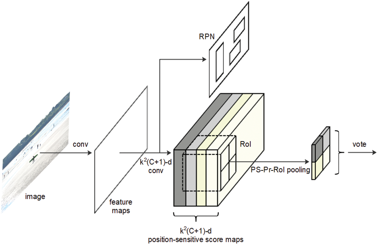
Figure 1: The overall precise R-FCN architecture

3.1 Precise R-FCN

The overall architecture for the presented detector can be divided into four parts: a basic convolutional neural network (ResNet-101) [34], an RPN [10], a position-sensitive score map layer (the last convolutional layer), and a PS-Pr-RoI pooling/voting layer [33].

3.1.1 Residual Networks

Residual networks are powerful tools that make training deeper networks possible. Prior to the development of residual networks, two potential problems arose as the number of network layers increased: decreasing accuracy and vanishing or exploding gradients [34]. Residual networks were developed to address these problems as their internal building blocks use shortcut connections that alleviate issues caused by increasing neural network depth. Each building block can be divided into two parts: shortcut connections and residual mappings. The building block formula is given by xl+1=f(y1), where yl=h(xl)+F(xl,Wl) and f(⋅) is an activation function that generally uses a rectified linear unit (ReLU). The term h(xl) describes shortcut connections, as shown in the lower part of Fig. 2, and F(xl,Wl) is a residual mapping that is generally composed of two or three convolution operations (displayed in the upper part of Fig. 2). In convolutional neural networks, the dimensions of xl may differ from that of xl+1, requiring the use of a 1×1 convolution to increase or reduce dimensionality. In this case, h(xl)=Wl′x, where Wl′x is a 1×1 convolution operation. When xl+1=xl+F(xl,Wl), the residual network exhibits several common attributes, including an L layer that can be expressed as the sum of any shallower layers and a corresponding residual component, which prevents vanishing gradients in the residual network. Finally, the gradient of the L layer can be transferred to that of any layer shallower than itself.

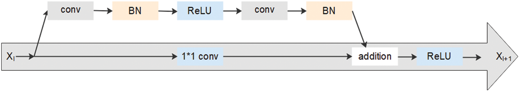
Figure 2: The building block. Here, the term addition refers to the unit addition operation and BN refers to the batch normalization

The residual network used in this study is a modified version of ResNet-101, developed by the authors of the R-FCN [33]. It included 100 convolutional layers, followed by a global average pooling layer, and a 1000-class fully connected layer [33]. After preserving 100 convolutional layers, we removed the global average pooling and fully connected layers, only using the convolutional layer to calculate feature maps [33]. We subsequently added a randomly initialized 1024-dimensional 1×1 convolutional layer to reduce the dimensionality and further utilize convolutional layers in the k2×(C+1) channel, to generate position-sensitive score maps [33].

3.1.2 Region Proposal Networks

RPNs can be used to generate RoIs for object detection. In a fast R-CNN [35], the entire image is sent to the CNN for the purpose of extracting feature maps. RoIs are then generated using an offline selection search algorithm. However, this process is time consuming and does not provide a clear methodology for generating RoIs. In contrast, RPNs are both efficient and concise as they incorporate RoI generation in end-to-end learning. Feature maps from the residual network are used as RPN input, while a set of rectangular proposals with an object score are produced as output [10]. As illustrated in Fig. 3, the RPN incorporates several key steps referred to as anchor generation, anchor object generation, RPN loss, and proposal generation.

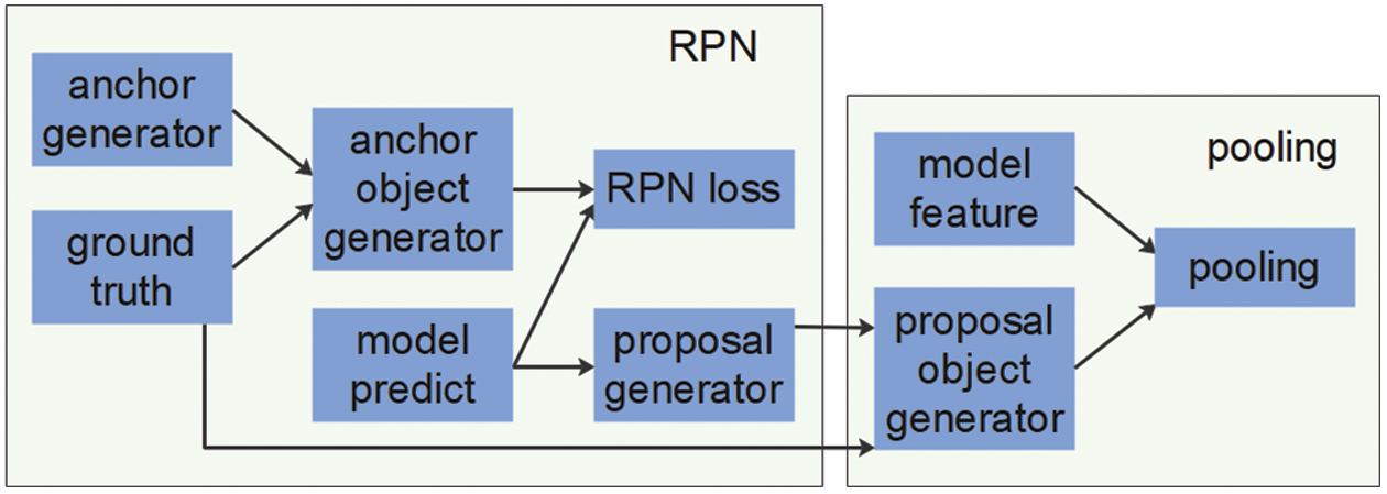
Figure 3: The region proposal network used to generate RoIs in the feature maps

Anchor generation: Anchors are preset using shared scale and ratio parameters. When an image of size 480×400 is input, using stride=16, the size of the feature map will be 30×25. The anchor scale is then (4,8,16) and the parameter ratio is (0.5,1,2). As a result, nine anchors are produced.

Anchor object generation: The anchor object layer differentiates positive and negative anchor samples. In this study, the intersection-over-union (IoU) was calculated between the anchor and the ground truth using three criteria. 1) For each ground truth, the anchor exhibiting the largest IoU overlap with a ground-truth box was selected as a positive sample. 2) Anchors exhibiting an IoU overlap higher than a certain threshold (T1) with any ground truth box were selected as positive samples. 3) If the IoU overlap with the ground truth box was less than a certain threshold (T2), the anchor was considered to be a negative sample. Anchors with an IoU value between T2 and T1 were labeled “do not care” samples that were not involved in RPN loss calculation or model optimization. These steps ensured that each ground truth was assigned a corresponding anchor and that a certain number of anchors could be selected to balance positive and negative samples.

RPN loss: Since RPNs include both classification and regression tasks, the corresponding loss term is comprised of both classification and regression loss. Cross-entropy loss was used for classification tasks while L1-smooth loss was used for regression tasks. These loss terms can be represented as:

L(s,tx,y,w,h)=Lcls(sc∗)+λ[c∗>0]Lreg(t,t∗) (1)

Lcls(sc∗)=−log⁡(sc∗) (2)

Lreg(t,t∗)=∑i∈{x,y,w,h}smoothL1(ti−ti∗) (3)

smoothL1(x)={0.5x2if |x|<1|x|−0.5otherwise (4)

where c∗ is an RoI ground truth label and t∗ represents the ground truth box.

Proposal generation: This step involves sorting by object score and inputting the first N1 terms to a non-maximum suppression (NMS) algorithm. The first N2 are then taken as the final output result after NMS is completed.

Fully convolutional networks are suitable for image classification applications due to their strong feature extraction capabilities. However, these networks focus solely on features and do not consider relative spatial positioning, making them unsuitable for object detection. In contrast, position-sensitive score maps can represent relative object locations. In this study, PS-Pr-RoI pooling was used to generate output of the same size from RoIs of different sizes, thereby producing a more accurate relative spatial position than that of RoI pooling [36]. This process does not quantize coordinates and is thus highly effective for eliminating localization misalignment and detecting small objects.

This approach can be described as follows. First, the original image is sent to a ResNet-101 [33] for feature map generation. An RPN and a convolutional layer are then used to acquire the k2×(C+1) and 4k2 position-sensitive score maps from the feature maps. PS-Pr-RoI pooling and voting operations are then performed on the maps to obtain classification and position information. The proposed small object detection algorithm based on a precise R-FCN is shown in Algorithm 1. Specific pooling and voting operations are described in detail as follows.

3.2 PS-Pr-RoI Pooling

In conventional RoI pooling, two quantization operations are performed on the RoI boundaries and bins, resulting in low position accuracy. RoI features are then updated without a gradient and thus cannot be adjusted during training. An RoI alignment step [37] can be used to eliminate quantization errors by canceling two quantization operations and using x/16 rather than [x/16]. This means that no quantization is performed on any coordinates involved in the RoI, its bins, or the sampling points [37]. The N sampling points within each bin were updated using bilinear interpolation with gradient conduction [37]. This produced a new parameter N, which is preset and cannot be adaptively adjusted according to the size of the bins. The gradient of these points is related to the features in the four integer positions surrounding them. Not all features in the bins possess a gradient.

Precise RoI pooling does not involve any quantization operations and solves problems associated with the number of sampling points by eliminating it as a system parameter [36]. In this study, all feature maps were made continuous through interpolation and the pooling operation was calculated using a two-order integral, to ensure all features exhibited gradient transfer. PS-Pr-RoI pooling, which includes clear relative spatial positioning, effectively improved the position sensitivity of deeper convolutional layers. In addition, it does not perform quantization operations on any coordinates, which eliminates localization misalignment. This approach improved detection accuracy for small objects.

Position-sensitive score maps: The position-sensitive score maps produced in the previous step contain clear relative spatial information, generated by the last convolutional layer. These maps include k×k colors (k=2 here for ease of explanation, k=7 in practical applications) that represent the probability of an object existing at specific locations. For instance, the gray map represents the probability of objects being present in the top-left position, while the light yellow map represents the probability of an object in the bottom-right position. Maps of each color include C+1 categories, including C object categories and a background category, for a total of k2×(C+1) points.

PS-Pr-RoI pooling: Each RoI was divided into k×k regular bins produced via PS-Pr-RoI pooling, regardless of its size. This pooling layer performed selective pooling, with each bin response collected from one of the k×k position-sensitive score maps [33]. The features in these maps were initially discretized and were made continuous at any coordinate (x,y) using bilinear interpolation, in order to perform PS-Pr-RoI pooling [36]. The score maps were also continuous as a result of the continuous features, which were calculated at any given coordinate (x,y) using:

f(x,y)=∑i,jIC(x,y,i,j)×wi,j (5)

Here, IC is an interpolation coefficient given by IC(x,y,i,j)=max(0,1−|x−i|)×max(0,1−|y−i|) and the feature wi,j is at a discrete position (i,j) in the map. Pooling was performed using:

PSPrPoolc(bin,F)=∫y1y2∫x1x2f(x,y)dxdy(x2−x1)(y2−y1) (6)

It is evident this function works to average all continuous features, yielding the pooled response in the (a,b)th bin for the cth category (0≤a,b≤k−1). Here, (x1,y1) is the top-left region of the bin, (x2,y2) is the bottom-right region of the bin, and the input F is one of the k2×(C+1) score maps. The PSPrPool function is continuously differentiable and its partial derivative x1 can be calculated using:

∂PSPrPoolc(bin,F)∂x1=PSPrPoolc(bin,F)x2−x1−∫y1y2f(x1,y)dy(x2−x1)(y2−y1) (7)

The input of the PS-Pr-RoI pooling is k2×(C+1) position-sensitive score maps. Following PS-Pr-RoI pooling, the position-sensitive score maps for different colors are formed into new k×k bins. For example, in Fig. 4, the gray map only occupies a bin at the top-left position, while the light yellow map is assigned to only the bin at the bottom-right position. Once all bins have been recombined, they take the form of a thin solid block shown on the right side of Fig. 4. This block forms the output of the PS-Pr-RoI pooling operation and has a dimension of C+1.

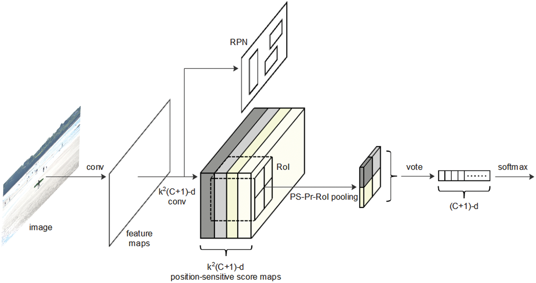
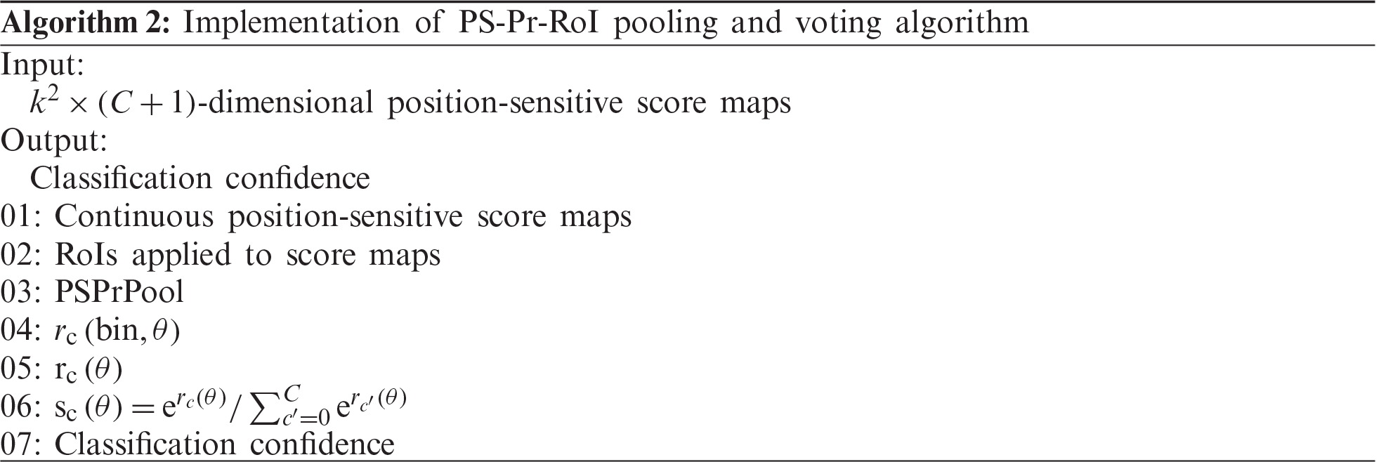
Figure 4: Implementation of PS-Pr-RoI pooling and voting operations

Voting: The output of the pooling step is used for voting. The k×k position-sensitive scores for each class are averaged directly [33] to produce a C+1-dimensional vector, given by:

rc(θ)=∑binrc(bin,θ) (8)

The position-sensitive object score for the cth category bin can be expressed as [33]:

rc(bin,θ)=PSPrPoolc(bin,F)=∫y1y2∫x1x2f(x,y)dxdy(x2−x1)(y2−y1) (9)

The C+1 softmax responses were calculated across categories and can be represented as follows:

sc(θ)=erc(θ)/∑c′=0Cerc′(θ) (10)

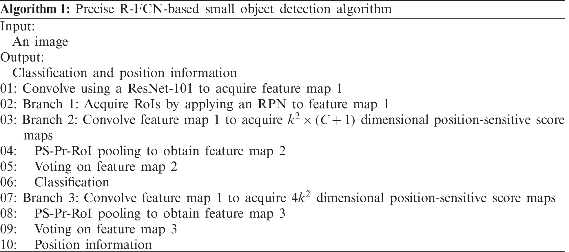
This term was used to calculate the cross-entropy loss during training and to rank RoIs during inference [33]. The PS-Pr-RoI pooling and voting steps are detailed in Algorithm 2.

Bounding box regression was defined in a similar way using a 4k2-dimensional convolutional layer. For each RoI, a 4k2-dimensional vector, used to parameterize a bounding box, was generated and then aggregated into a four-dimensional vector by average voting.

4  Experimental Results and Analysis

Detection performance was evaluated experimentally for small objects using the mean average precision (mAP) metric, as shown in Fig. 5.

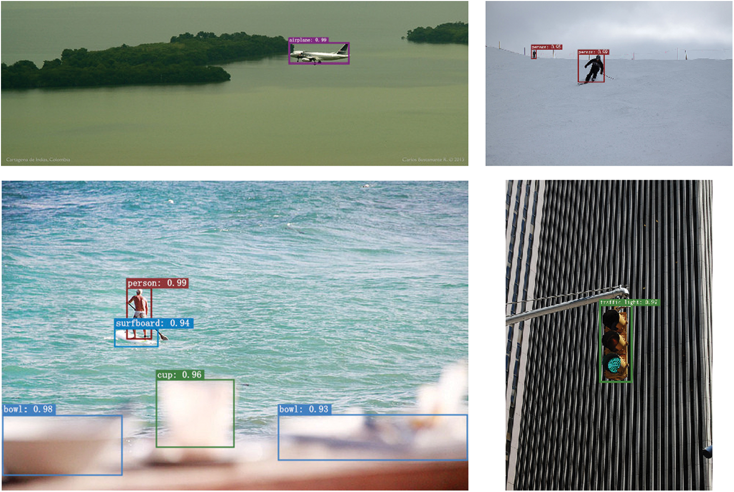
Figure 5: Precise R-FCN results for the COCO test-dev datasets. These results are based on a ResNet-101, achieving an AP of 32.9. The bounding box, classification, and confidence values are also included

4.1 Experimental Environment

The validation experiment included a GPU utilizing an Nvidia GeForce GTX TITAN X. The convolutional neural network environment and configuration were as follows. All detectors in the experiment were run on Ubuntu 16.04 using the TensorFlow deep learning framework and CUDA (version 10.1) programmed with Python 3.7.

4.2 Implementation Details

The accuracy of the detector was evaluated using MS COCO datasets containing a total of 80 objects. By default, we used a single-scale training and testing step, following a process similar to that of Kisantal et al. [15] for processing the training data. Multiple image copies were created that contained small objects (using a preset sampling ratio of 3), rather than performing a random oversample [15]. ResNet-101 was used as the basic convolutional neural network, pre-trained with ImageNet [38]. The ResNet’s effective stride was reduced from 32 to 16 pixels to increase the resolution of the position-sensitive score maps and improve the accuracy of small object detection. All layers before and at the conv4 stage remained unchanged and the RPN was computed on top of the conv4 stage [33]. The RPN was used to identify RoIs, defined as positive samples with an IoU overlap of at least 0.5 with a ground truth box. Other samples were deemed negative. N3 proposals were calculated for each image during the forward pass and the corresponding loss was also evaluated. In addition, the 128 sample RoIs with the highest loss were selected for backpropagation [33]. A total of 300 RoIs were used for testing [10] and were post-processed by NMS using a threshold of 0.3 IoU. The loss functions defined for each RoI are shown in Eqs. (1)–(4). The balance weight was set to λ=1 and c∗>0 requires RoIs to be in the foreground. PS-Pr-RoI pooling was then applied with a momentum of 0.9 and a weight decay of 0.0005. The stochastic gradient descent (SGD) [39] method was implemented to identify optimal solutions by training the loss function.

4.3 Results and Analysis

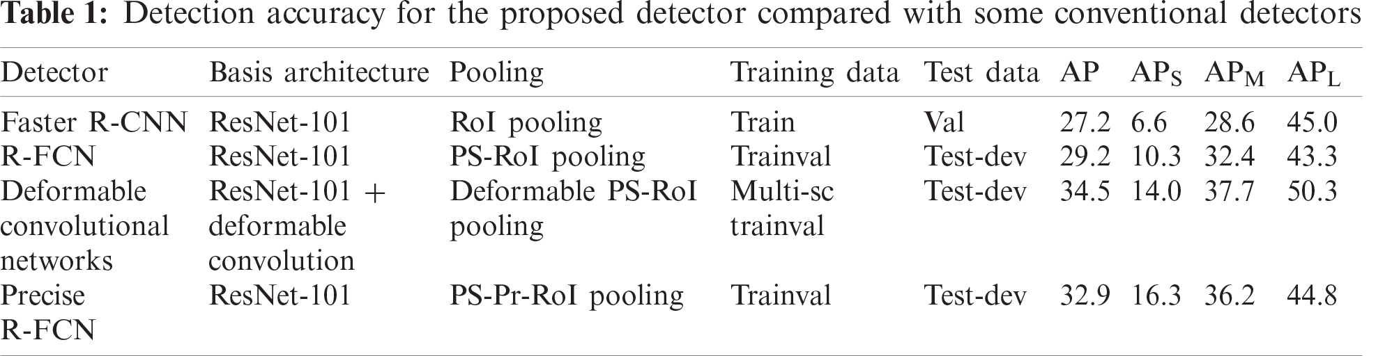
The proposed detector is simple and requires no additional features, such as multi-scale training or testing. In addition, with the aid of PS-Pr-RoI pooling, our detector can increase object detection accuracy beyond that of some conventional algorithms. Tab. 1 shows average precision (AP) values for IoU=0.5:0.05:0.95. The APS, APM, and APL terms represent detector AP measurements for small, medium, and large objects, respectively. As seen in the table, the proposed detector achieved substantial improvements in performance compared with Faster R-CNN and R-FCN, as measured by APS, APM, and APL. This is primarily due to the inclusion of a novel PS-Pr-RoI pooling module that eliminates localization misalignment, by not involving any quantization of coordinates, and the use of features exhibiting gradient transfer. This PS-Pr-RoI pooling can effectively improve position sensitivity for deeper convolutional layers as it includes a relative spatial position. Notably, deformable convolutional networks [40] outperformed our detector as measured by AP, through the use of deformable convolutions, deformable PS-RoI pooling, and a multi-scale training strategy. However, our approach produced a superior APS value, demonstrating that PS-Pr-RoI pooling can improve the detection of small objects.

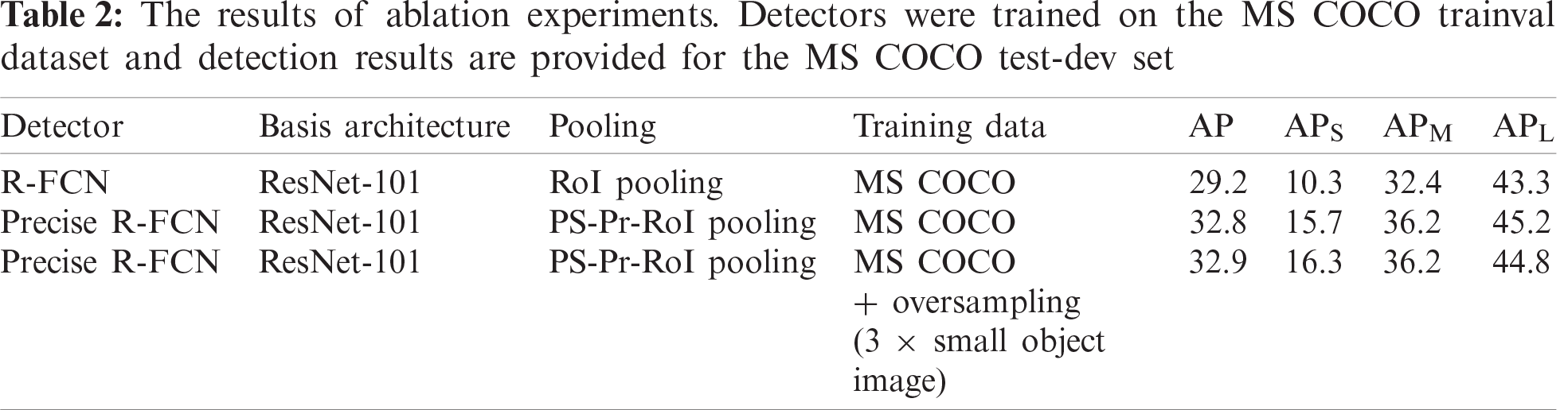
Ablation experiments: In this study, PS-Pr-RoI pooling is proposed as a replacement for PS-RoI pooling in an R-FCN. Our approach was found to not only improve AP but also to significantly improve APS for the processed training datasets. This is a useful way of solving the problem of large and small object imbalances in training datasets such as MS COCO [15]. Tab. 2 displays the accuracy achieved by the same detector for various training data. Experimental results showed this strategy improved the APS index but decreased the APL index. One possible explanation is that the training datasets were preprocessed, adding a large number of images containing small objects. This increased the contribution of small objects to computational loss, which biased the overall network towards small object detection and thus resulted in a decrease in APL.

5  Conclusion

In this study, the accuracy of small object detection was improved and localization misalignment was eliminated using PS-Pr-RoI pooling. This pooling module was embedded in a two-stage detector R-FCN, which greatly increased detection accuracy for small objects. In a future study, we intend to combine PS-Pr-RoI pooling with other detectors for use in other types of image research [41]. Other detector frameworks could also be easily integrated with the studied module for increased object detection accuracy.

Funding Statement: This project was supported by the National Natural Science Foundation of China under grant U1836208, the Hunan Provincial Natural Science Foundations of China under Grant 2020JJ4626, the Scientific Research Fund of Hunan Provincial Education Department of China under Grant 19B004, the “Double First-class” International Cooperation and Development Scientific Research Project of Changsha University of Science and Technology under Grant 2018IC25, and the Young Teacher Growth Plan Project of Changsha University of Science and Technology under Grant 2019QJCZ076.

Conflicts of Interest: The authors declare that they have no conflicts of interest to report regarding the present study.

This work is licensed under a Creative Commons Attribution 4.0 International License, which permits unrestricted use, distribution, and reproduction in any medium, provided the original work is properly cited.