Computers, Materials & Continua DOI:10.32604/cmc.2021.017516
Article

Outlier Detection of Mixed Data Based on Neighborhood Combinatorial Entropy

Lina Wang1,2,*, Qixiang Zhang1, Xiling Niu1, Yongjun Ren3 and Jinyue Xia4

1School of Artificial Intelligence, Nanjing University of Information Science and Technology, Nanjing, 210044, China
2Southern Marine Science and Engineering Guangdong Laboratory (Zhuhai), Zhuhai, 519080, China
3School of Computer and Software, Nanjing University of Information Science and Technology, Nanjing, 210044, China
4International Business Machines Corporation (IBM), New York, 10504, USA
*Corresponding Author: Lina Wang. Email: wangln@nuist.edu.cn
Received: 02 February 2021; Accepted: 10 April 2021

Abstract: Outlier detection is a key research area in data mining technologies, as outlier detection can identify data inconsistent within a data set. Outlier detection aims to find an abnormal data size from a large data size and has been applied in many fields including fraud detection, network intrusion detection, disaster prediction, medical diagnosis, public security, and image processing. While outlier detection has been widely applied in real systems, its effectiveness is challenged by higher dimensions and redundant data attributes, leading to detection errors and complicated calculations. The prevalence of mixed data is a current issue for outlier detection algorithms. An outlier detection method of mixed data based on neighborhood combinatorial entropy is studied to improve outlier detection performance by reducing data dimension using an attribute reduction algorithm. The significance of attributes is determined, and fewer influencing attributes are removed based on neighborhood combinatorial entropy. Outlier detection is conducted using the algorithm of local outlier factor. The proposed outlier detection method can be applied effectively in numerical and mixed multidimensional data using neighborhood combinatorial entropy. In the experimental part of this paper, we give a comparison on outlier detection before and after attribute reduction. In a comparative analysis, we give results of the enhanced outlier detection accuracy by removing the fewer influencing attributes in numerical and mixed multidimensional data.

Keywords: Neighborhood combinatorial entropy; attribute reduction; mixed data; outlier detection

1  Introduction

Outlier detection is frequently researched in the field of data mining technologies and is aimed at identifying abnormal data from a data set [1]. It is widely applicable for credit card fraud detection, network intrusion detection, fault diagnosis, disaster prediction, and image processing [2–8]. Presently, outlier detection methods are conducted with statistical techniques [9], which include distance-based proximity, network-based and density-based proximity [10–12], data clustering [13], and rough set data modeling [14].

Statistical methods require the presence of a single feature and predicable data distribution. In real environment, many data distributions are unpredictable and multi-featured. In addition, their applications are restricted [15]. Knorr et al. [16] proposed a distance-based method that required little information of the data set and was therefore suitable for any data distribution. Early outlier detection algorithms focused on mining global outliers. Contrarily, a multidimensional algorithm must outline data locally because its data sets are unevenly distributed, complex, and difficult to identify. Since Breunig et al. [10] put forward the concept of local outliers, local outlier detection has attracted considerable attention owing to its practical advantage in reducing time overhead and improving scalability. The local outlier detection algorithm starts by calculating the outlier value of local data and defining outlying data. Subsequently, the local outlier detection algorithm focuses on the local neighborhood determination to calculate local outliers [17,18]. A clustering algorithm divides a data set into several clusters to show similarities and differences of objects based on their respective clusters [19]. When judging a local outlying object, a cluster is considered as its neighborhood, and the local outliers of the data are calculated in the neighborhood [20]. Outlier detection based on information entropy theory [21] judges the amount of information in the outlier through entropy value and determines outlying data in light of their entropies [22]. The introduction of information entropy weighting effectively improved the outlier detection accuracy [23].

Many studies [24–27] focused on rough set-based detection methods, which originated from intelligent systems. Although the studies provided insufficient and incomplete information, they were introduced into outlier detection to handle categorical data. Conventional outlier detection uses more numerical data than classical rough set-based methods as they deal with categorical data. However, the processing of mixed data of categorical and numerical attributes, ubiquitous in real applications, has received inadequate attention. Through the adoption of robust neighborhood, explorations were conducted to improve classical rough sets for better performance in numerical and mixed data. At present, neighborhood rough sets are effective for attribute reduction, feature selection, classification recognition, and uncertainty reasoning.

This study aims to use a novel approach by combining attribute reduction with outlier detection technology to improve the outlier detection accuracy, reduce calculation complexity, remove fewer influencing attributes and reduce data dimensions. Data-processing plays a significant role in attribute reduction by using experimental multi-type data to achieve an accuracy boost for outlier detection. Using the neighborhood combinatorial entropy model, we construct mixed data outlier detection algorithms after defining the local outlier factor (LOF) algorithm, neighborhood combinatorial entropy algorithm and relevant concepts. Comparative data analysis is conducted to verify the detection accuracy after attribute reduction.

The rest of the paper is structured as follows. Section 2 provides the LOF algorithm, providing related definitions. Section 3 discusses the neighborhood combinatorial entropy algorithm, providing related definitions. Section 4 constructs the mixed data outlier detection algorithms based on neighborhood combinatorial entropy. Section 5 carries out the experimental analysis on the advantages of attribute reduction prior to outlier detection. Finally, Section 6 concludes the paper.

2  Local Outlier Factor Algorithm

2.1 Related Definitions

The LOF algorithm is a representative outlier detection algorithm that computes local density deviation [10]. It calculates a local outlier factor of each object, and judges whether the object is an outlier that deviates from other objects or a normal point.

Definition 1: We define the distance (Euclidean distance) between object x and object y; two objects in object set U are as follows:

d(x,y)=∑i=1m(xi−yi)2, (1)

where m represents the dimension of the objects; and xi and yi represent the coordinates of the ith dimension of objects x and y, respectively.

Definition 2: We define the kth nearest distance of an object x in object set U as:

dk(x)=d(x,p), (2)

where p is the kth nearest neighbor to object x in all dimensions (excluding object x). The Euclidean distance between object x and object p is the kth nearest distance of object x. As shown in Fig. 1, the object y5 is the 5th closest neighbor to the object x, which concludes that d5(x)=d(x,y5).

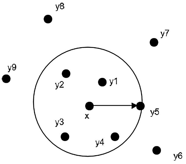
Figure 1: The 5th nearest neighbor of object x

To determine the value of k, the number of objects in the set satisfies the following: (1) the number of objects q (object x excluded) is at least k so that d(x,q)≤d(x,p); (2) the number of object q (object x excluded) is at most k−1, making d(x,q)≤d(x,p).

Definition 3: We define the neighborhood of k nearest neighbors of the object x in object set U as:

Nk(x)={y∣y∈U,d(x,y)≤dk(x)} (3)

Eq. (3) describes the set of objects within the kth nearest distance (including the kth nearest distance) of the object x; therefore, the number of objects in the neighborhood of x conforms to |Nk(x)|≥k. As shown in Fig. 1, the 5 nearest neighbors of object x are the set {y1,y2,y3,y4,y5}.

Definition 4: We define the kth reachable distance from the object x to object p in object set U as:

R_distk(x,p)=max{dk(x),d(x,p)} (4)

The kth reachable distance from x to p is longer between the kth nearest distance of x and real distance from x to p. The distances from x to the k-nearest objects from x are equal and are dk(x). The distance between the object x and other objects apart from the above-mentioned k nearest objects is the real distance between the two objects.

As indicated in Fig. 2, the actual distance from x1to p is smaller than the 5th nearest distance of x1. From the definition, R_dist5(x1,p)=d5(x1). The actual distance from x2 to p is greater than the 5th nearest distance from x2; thus, R_dist5(x2,p)=d(x2,p).

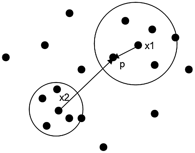
Figure 2: The 5th reachable distances from x1 and x2 to p

Definition 5: We define the local reachable density of the object x in object set U as:

LRDk(x)=|Nk(x)|∑y∈Nk(x)R_distk(x,y) (5)

LRDk(x) refers to the density. The larger the value LRDk(x), the higher the density, and the more the objects belong to the same cluster. Contrarily, the smaller the value LRDk(x), the lower the density, revealing that the objects are likely to be outliers.

If the object x is in the same cluster as the neighboring objects, the reachable distance is likely to be dk(x), the kth nearest distance of the object x. Otherwise, the reachable distance may be d(x,y), which is the true distance. From Eq. (4), dk(x), the kth nearest distance of object x is smaller than d(x,y), the true distance. Hence the denominator of Eq. (5) in the same cluster is smaller than that in different clusters. The values LRDk(x) in the same cluster will be larger than those in different clusters. When the value LRDk(x) is smaller, object x is likely to be an outlier.

Definition 6: We define the local outlier factor of the object x in object set U as:

LOFk(x)=∑y∈Nk(X)LRDk(y)LRDk(x)|Nk(x)| (6)

LOFk(x) represents the average ratio of the local reachable density of the objects in the neighborhood Nk(x) and the object x to the local reachable density of the object x. When the value LOFk(x) is closer to 1, the local reachable density of the objects in the neighborhood Nk(x) is closer to the local reachable density of the object x. The object x is likely to be in the same cluster in its neighborhood. Otherwise, when the value LOFk(x) is smaller than 1, the local reachable density of the object x is higher than that of its neighborhood, revealing that the object x tends to be in the dense points. If the value LOFk(x) is larger than 1, the local reachable density of the object x is lower than that of its neighborhood, revealing that the object x is likely to be an outlier.

2.2 Analysis of LOF Algorithm

The LOF algorithm examines whether the point is an outlier, which is carried out by comparing the local density of each object x and its neighboring objects. The lower the density of object x, the more likely it is an outlier. The density is calculated using the distance between objects. The farther the distance, the lower the density, and the higher the outlier. In certain objects, the neighborhood of k nearest neighbors is introduced to expand its global determination as a substitute to direct global calculation. In this way, one or more clusters of dense points are determined based on local density, thereby realizing multiple clusters identification. The cluster is comprised of multi-type data, containing categorical attribute, numerical attribute or mixed attribute. However, the algorithm of Eq. (1) can only process numerical data. The accuracy of LOF algorithm is ineffective for categorical or unknown data types.

3  Neighborhood Combinatorial Entropy

The neighborhood combinatorial entropy calculation follows two aspects: neighborhood approximate accuracy and neighborhood conditional entropy. The neighborhood approximate accuracy is the ability to divide the system from the set perspective [28,29]; whereas, the neighborhood conditional entropy is the ability to divide the system from the knowledge perspective [30].

3.1 Related Definitions

The information system is an aspect of data mining, expressed in a four-dimensional form IS=(U,A,V,f). In this system, U={x1,x2,…,xn} is a non-empty limited set of objects; A={a1,a2,…,al} is a non-empty set of attributes; V is the union of the attribute domain Va; and f is the information function: U∗A→V, which is ∀x∈U,∀a∈A,f(x,a)∈Va.

In addition, attributes are categorized into conditional and decision attributes. Therefore, attribute set A is the union of conditional attribute set C and decision attribute set D, namely, A=C∪D. Moreover, the information system is defined as a decision-making system DS=(U,C∪D,V,f).

When neighborhood range is set manually, δ, a neighborhood threshold is added to the information system and transformed into a neighborhood information system NI=(U,A,V,f,δ). In this case, δ is also called the neighborhood radius.

Definition 7: We define the distance measure of two objects on attribute subset B⊆C as:

DistB(x,y)=∑i=1mdai2(x,y)(1≤i≤m) (7)

In Eq. (7), B={a1,a2,…,am} is a subset of attributes,

where

m represents the dimension of the object, namely, the number of attributes.

ai corresponds to the ith attribute.

x and y are in U.

dai2(x,y) is the square of the distance between object x and object y in the ith dimension.

The calculations on the distance between two objects are different, which depend on attribute types [31],

where

ai is a numerical attribute; and

dai(x,y)=|x−y|max(ai)−min(ai). (8)

By eliminating the influence of dimension and value range between the attributes, numerical attributes are pre-processed into dimensionless data where each attribute value falls within the range of [0, 1]

where

ai is categorical attribute; and

dai(x,y)={1,xai≠yai0,xai=yai. (9)

Categorical data are converted into numerical data, and their values are determined per their categories. From Eq. (8), the data values of all numerical attributes are within the range of [0, 1]. Thus, we set the maximum value of the distances of different types to 1, and that of the minimum value to 0. After converting categorical data into numerical data, the distance between different objects is obtained through numerical calculations

where

ai is an unknown attribute; and

dai(x,y)=1. (10)

Eq.(10) is a new classification due to the unknown attribute. The data in this category belongs to a cluster different from other data, and a maximum distance of 1 is defined according to different attribute classifications in the clusters.

When processing different data categories, corresponding formulas are selected. Subsequently, the distance of the mixed data is obtained by applying Eq. (7), and the application of mixed data is realized by adopting different distance calculation following different attribute types.

DistB(x,y) becomes the effective distance in the neighborhood information system. When combined with neighborhood threshold parameter δ, it defines neighborhood relationship.

Definition 8: In a neighborhood information system NI=(U,A,V,f,δ), the neighborhood of object x on attribute subset B is:

NBδ(x)={y∣x,y∈U,DistB(x,y)≤δ} (11)

Definition 9: We define the upper approximation and lower approximation of the attribute subset B in an object set X, X⊆U as:

NUBδ(x)={x∈U∣NBδ(x)∩X≠∅} (12)

NDBδ(x)={x∈U∣NBδ(x)⊆X} (13)

Their relationship is expressed in Fig. 3.

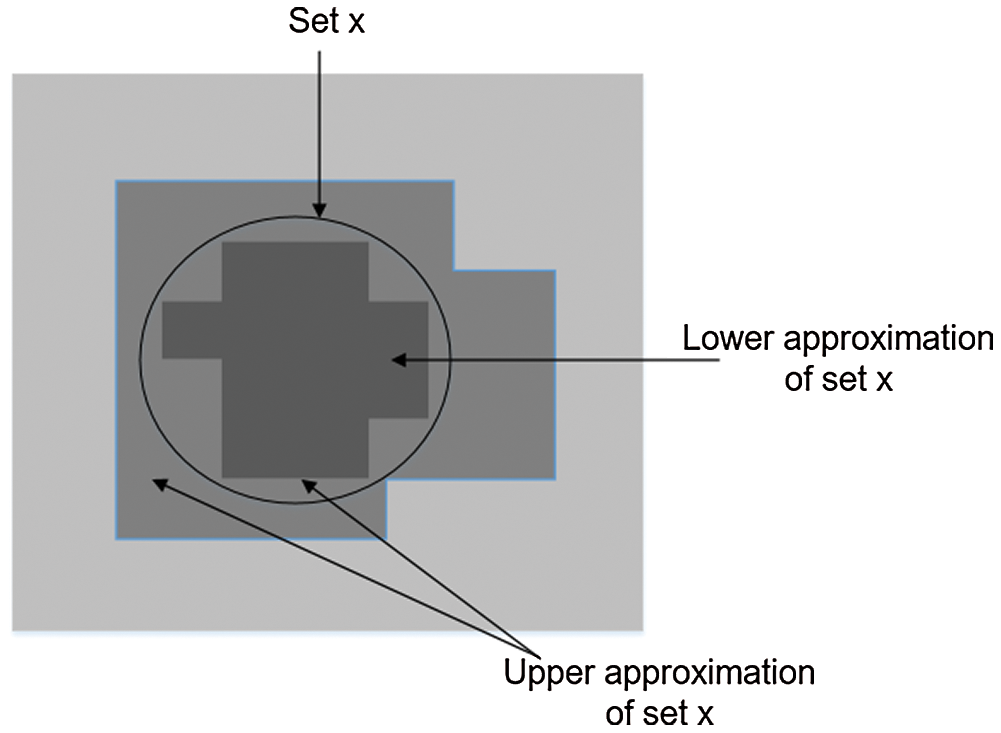
Figure 3: Conceptual diagram of upper and lower approximations

Definition 10: We divide the object set U into UD={D1,D2,…,Dm} according to its decision attributes. The approximate accuracy of the neighborhood of attribute subset B is:

αBδ(D)=∑i=1mNDBδ(Di)∑i=1mNUBδ(Di) (14)

As shown in Fig. 3, NDBδ(x)⊆NUBδ(x), so 0≤αBδ(D)≤1. Compared with the upper approximation, the lower approximation of the set X increases more significantly similar to the set B. Similarly, the value of the neighborhood approximation accuracy αBδ(D) increases. However, in a probability, as the attribute subset B increases, the increase of the lower approximation in the set X is equal to that of the upper approximation in the set X. Therefore, the value of αBδ(D), the neighborhood approximate accuracy, remains unchanged. This case has no impact on the final result (refer to Definition 13 for a detailed analysis).

Definition 11:We define the neighborhood information entropy of attribute subset B in the object set U as:

NE(B)=1−1|U|∑i=1|U||NBδ(xi)||U| (15)

|NBδ(xi)||U| represents the affiliation of the object xi in the neighborhood NBδ(xi) and 0≤|NBδ(xi)||U|≤1. Neighborhood entropy simulates the classic information entropy and provides an overall uncertainty description for neighborhood information. As the neighborhood information entropy of a certain attribute subset grows larger, this attribute subset distinguish different objects in the set U, particularly when B=∅ and NE(∅)=0.

Definition 12: We define the neighborhood conditional entropy of attribute set Q, P⊆C under the condition of P as:

NE(Q∣P)=NE(Q∪P)−NE(P)=1|U|2∑i=1|U|(|NPδ(xi)|−|NQδ(xi)∩NPδ(xi)|) (16)

Since P⊆C is for attribute set Q, attribute set C is a conditional attribute, and Q and P are conditional attribute sets. Eq. (16) reflects the uncertainty of conditional attribute set P to conditional attribute set Q. If Q is a set of decision attributes D, NE(D∣P) represents the uncertainty of a set of conditional attributes P to a set of decision attributes D. The entropy value of neighborhood conditional entropy is monotonous and bounded, and its value decreases as the conditional attribute set P increases.

Definition 13: We divide the object set U into UD={D1,D2,…,Dm} based on its decision attribute. The neighborhood combinatorial entropy of Di on attribute subset B is defined as:

NCEBδ(Di)=αBδ(Di)NE(Di∣B) (17)

From Eq. (17), neighborhood combinatorial entropy is composed of Eqs. (14) and (16), reflecting uncertainties in set theory and knowledge, respectively. Thus, neighborhood combinatorial entropy interprets uncertainty from multiple angles, and its uncertainty is more comprehensive than that in either set theory or knowledge.

Though αBδ(Di), the neighborhood approximation accuracy in Definition 10 is non-monotonic and does not exert influence on the final neighborhood combinatorial entropy. αBδ(Di) increases or remains unchanged as the attribute subset B increases. However, neighborhood conditional entropy affects the result of neighborhood combinatorial entropy. Analysis in Definition 12 shows that neighborhood conditional entropy has strict monotonicity. Though αBδ(Di) remains constant in some cases, the neighborhood combinatorial entropy maintains its monotonicity.

From the above analysis, αBδ(Di) increases or remains unchanged as attribute subset B increases. In Eq. (17), the neighborhood conditional entropy NE(Di∣B) decreases as the attribute subset B increases, and the neighborhood combinatorial entropy NCEBδ(Di) increases as the attribute subset B increases. With changes in conditional attribute set, the higher the neighborhood combinatorial entropy value for a conditional attribute set, the more important a conditional attribute is to the whole system.

Definition 14: We define the significance of a conditional attribute al∈C−B (attribute subset B excluded) to attribute subset B as:

Sig(al,B,D)=NCEB∪alδ(D)−NCEBδ(D) (18)

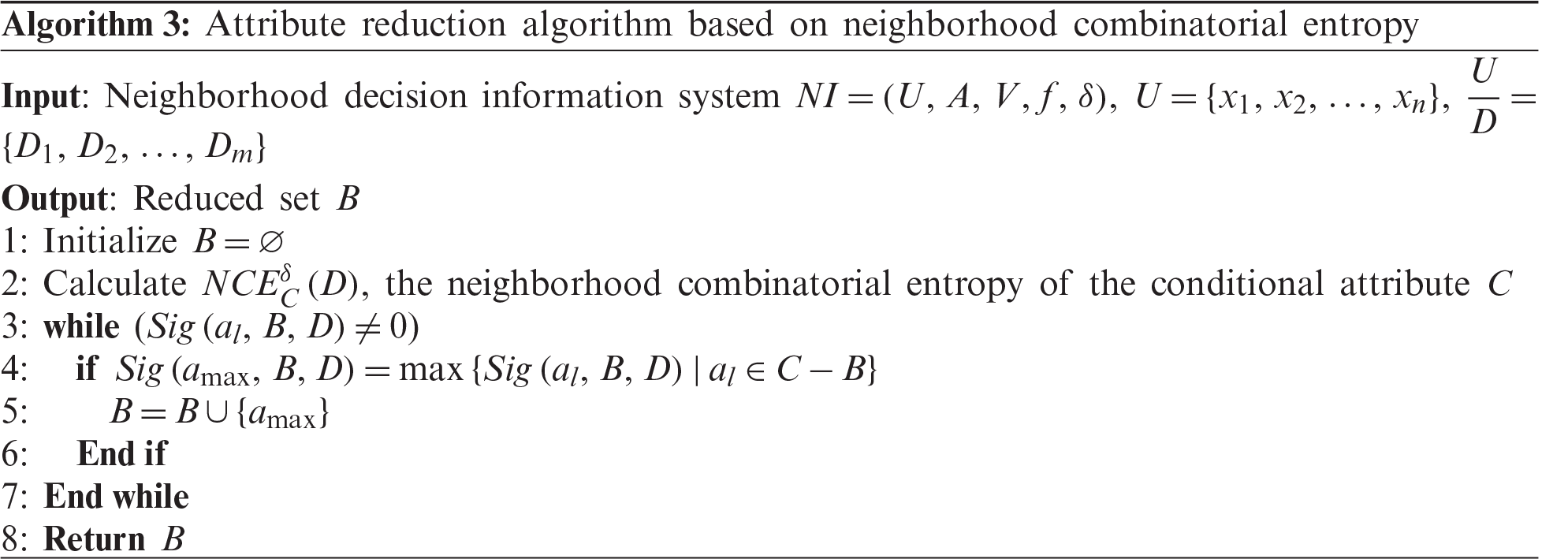
First, we set an attribute subset as an empty set. Then, we compare all conditional attributes {a1,a2,…,am} according to Eq. (18). If Sig(al,B,D) takes the maximum value of Sig(al,B,D) of all conditional attributes except the attribute subset B, the conditional attribute has the highest significance of all the conditional attributes except set B, written into attribute subset B. By iterative procedure, more conditional attributes are obtained in descending order of significance. Based on a threshold value of significance, conditional attributes are kept in the attribute subset B; otherwise, they are removed. When this procedure is completed, a data set of the attribute reduction is available.

3.2 Analysis of Neighborhood Combinatorial Entropy

From an information theory perspective, an entropy value reflects the importance of a condition attribute in an information system in determining whether the condition attribute is reduced. Entropy has the following properties: non-negativity, i.e., H(X)≥0; and maximum value, i.e., H(p1,p2,…,pn)≤H(1n,1n,…,1n)=log⁡n, reflecting a measure of significance in both the set and knowledge and the uncertainty of the set and knowledge. Therefore, the measurement of significance is a multi-angle operation.

4  Mixed Data Outlier Detection Algorithm Based on Neighborhood Combinatorial Entropy

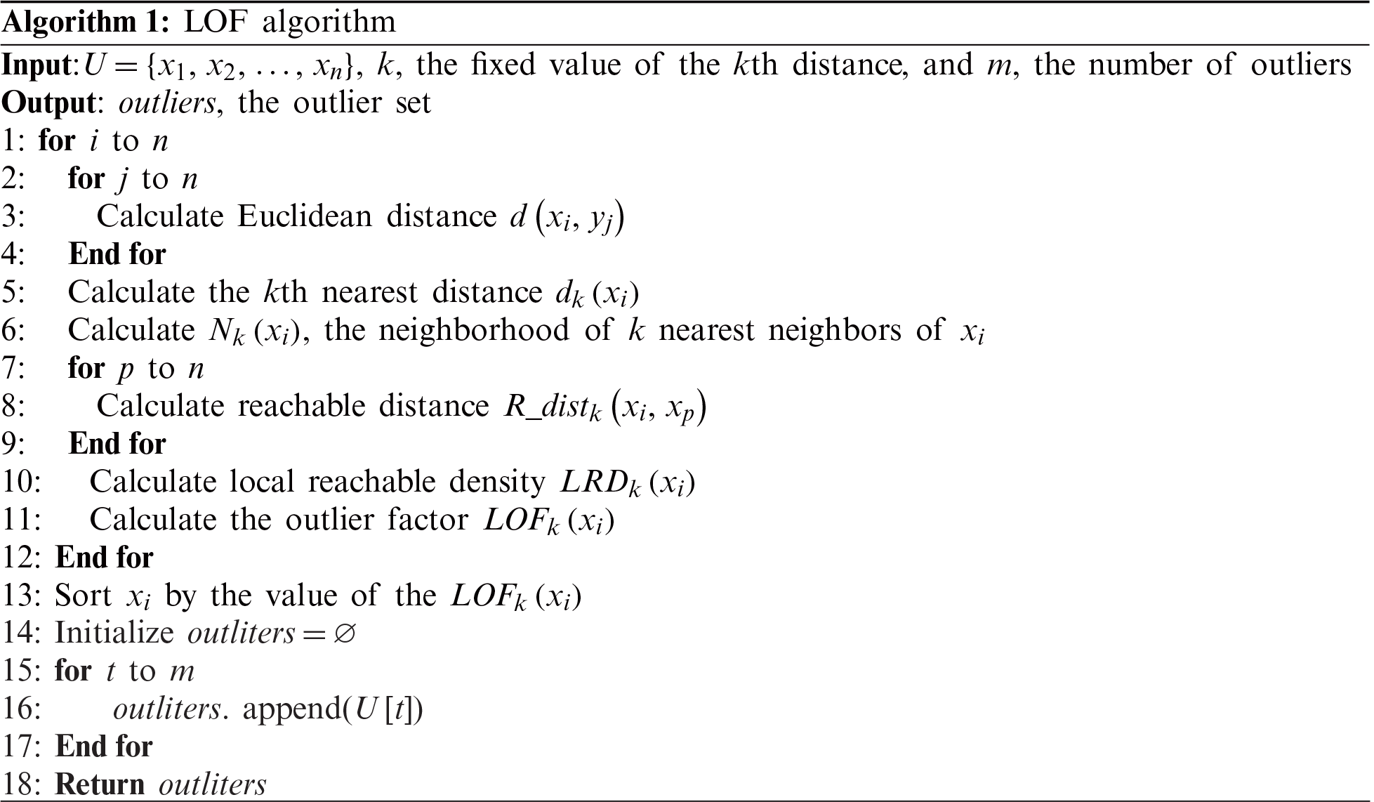
In Algorithm 1, the LOF algorithm focuses on estimating Euclidean distance. Higher data dimension implies more squares and longer calculation time. In the LOF algorithm, a lower data dimension saves significant calculation time.

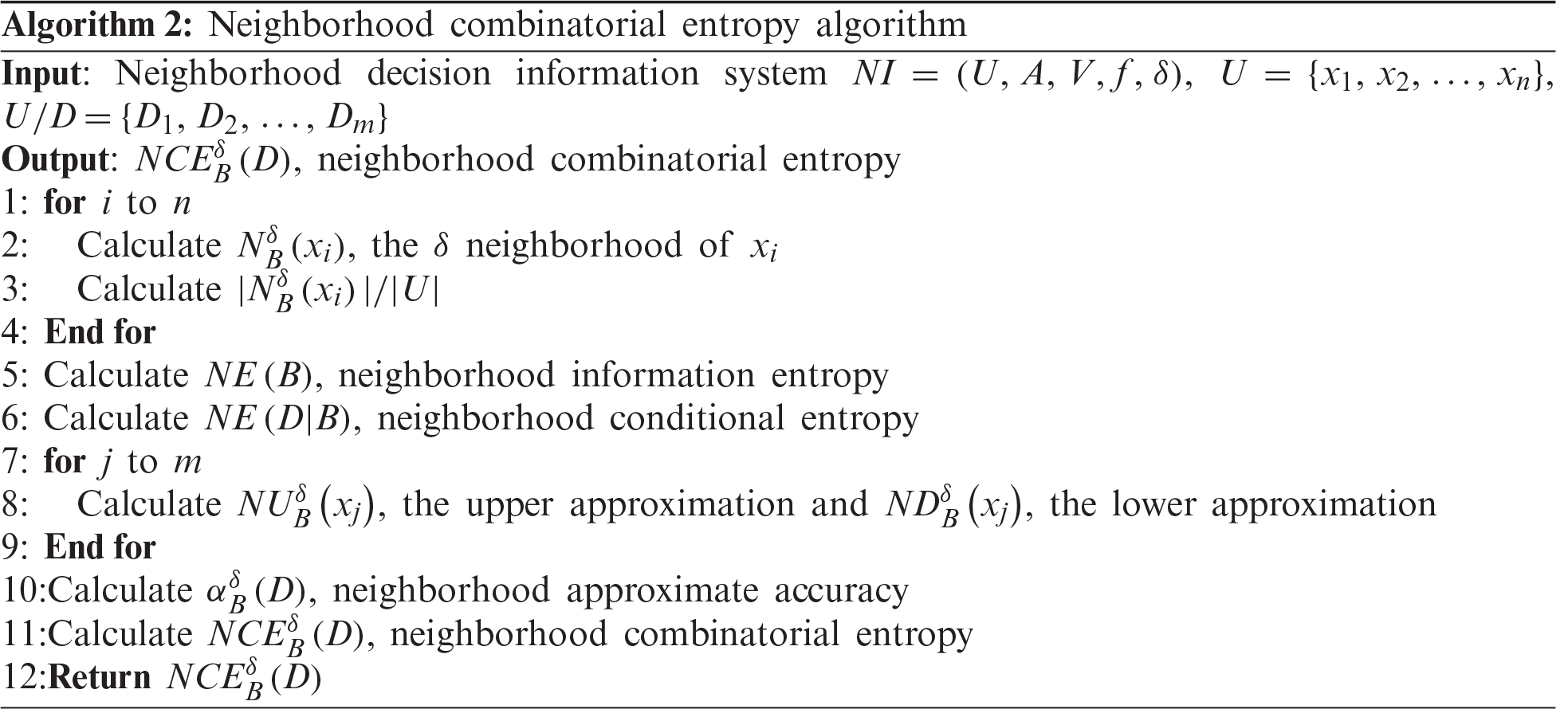
Algorithm 1 has limited capability for mixed data outlier detection. Algorithm 2 adopts different calculation methods for different attribute. Categorical and mixed data participate in data operation. After data treatment with Algorithm 3, attribute-reduced data are obtained and processed with LOF algorithm (Algorithm 1).

Attribute reduction filters out redundant data and shortens the calculation time without altering system applicability as some attributes are redundant and cause errors in the system. Filtering out errors improves the system’s accuracy. In Algorithm 2, neighborhood combinatorial entropy determines the significance of a conditional attribute in the attribute subset of the entire system. Applying Algorithms 2, 3 and the LOF algorithm for data processing reduces the data size processed by outlier detection, improve the outlier detection accuracy, and reduce misjudgment proportion.

5  Experimental Analysis

5.1 Experimental Data Set

5.1.1 220 Randomly Generated 2-Dimensional Data

First, 100 2-dimensional data of normal distribution are first randomly generated. To verify the LOF algorithm detection ability, the 100 random data are translated separately to form two clusters of data widely apart from one another. Hence, 200 data are generated. As presented in Fig. 4a, all dense points are divided into two clusters. The distribution of outliers is shown in Fig. 4b; blue dots are the 200 dense data, and yellow dots are the 20 outliers. The outlier points are relatively far from the two clusters of dense points, providing better references and contrast for the experiment on Algorithm 1.

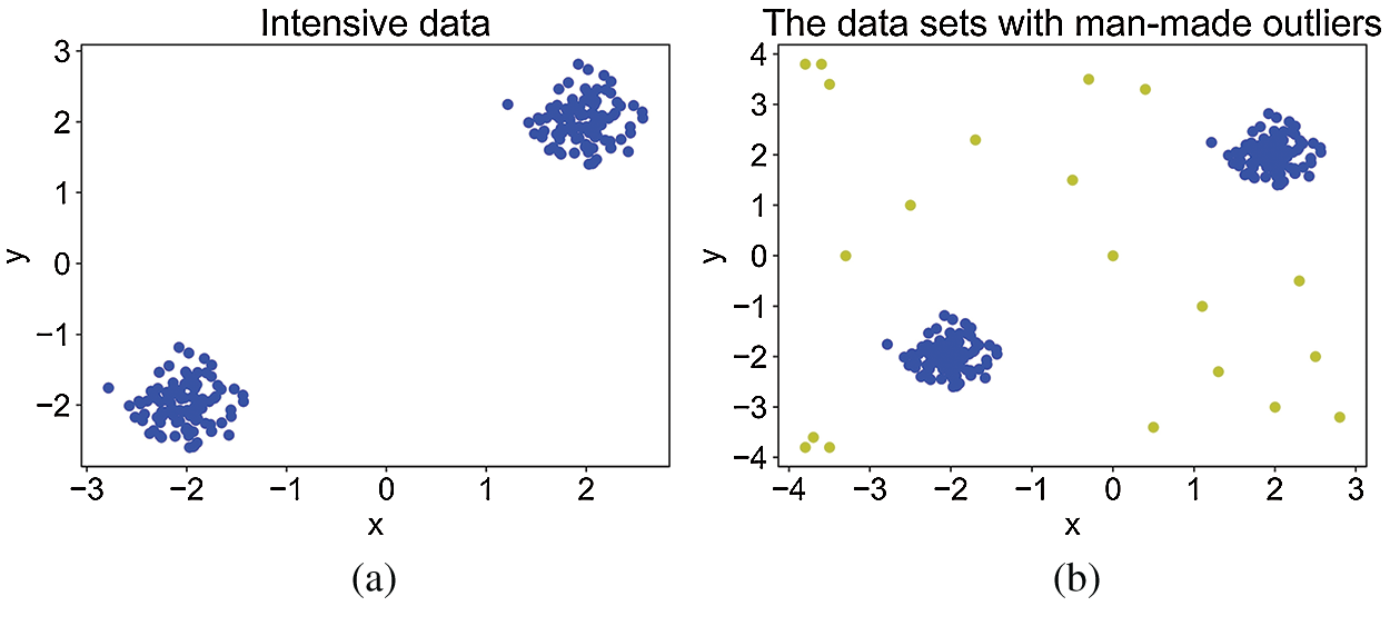
Figure 4: Two clusters with 2-dimensional attributes: (a) dense points (b) points with man-made outliers

5.1.2 220 Randomly Generated 8-Dimensional Data

A total of 200 8-dimensional dense data and 20 8-dimensional outlier data are randomly generated. The method generating the data is as same as that generating the randomly 2-dimensional data.

5.1.3 220 Randomly Generated 16-Dimensional Data

A total of 200 16-dimensional dense data and 20 16-dimensional outlier data are generated as the outlined in Fig. 4.

5.1.4 Wisconsin Breast Cancer Data Set

The Wisconsin breast cancer data set contains 699 objects with 10 attributes. From the 10 attributes, 9 attributes are numerical conditional attributes, and 1 is a decision attribute. All cases are in two categories: benign (458 cases) and malignant (241 cases). Some malignant examples are removed to form an unbalanced distribution of all the data, assisting the experimental data in accordance with the cases of few outliers in practical applications. The data set contains 444 benign instances (91.93%) and 39 malignant instances (8.07%). Fig. 5 presents the results of malignant objects as outliers.

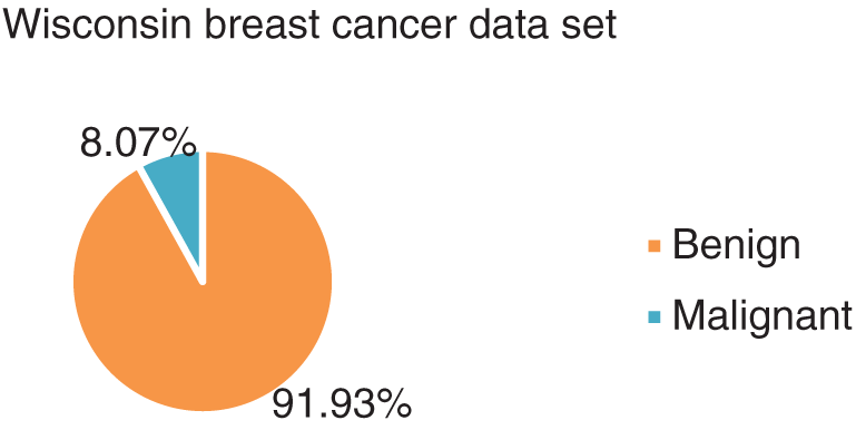
Figure 5: The distribution pie chart of the Wisconsin breast cancer data set

5.1.5 Annealing Data Set

The annealing data set contains 798 objects with 38 attributes. Among the 38 attributes, 30 are classified condition attributes, 7 are numerical condition attributes, and 1 is decision attribute. The 798 objects are in 5 categories. The first category contains 608 objects (76.19%), and the remaining 4 categories contain 190 objects (23.81%). Classes 2–5 are all regarded as outliers. The distribution is visualized in Fig. 6.

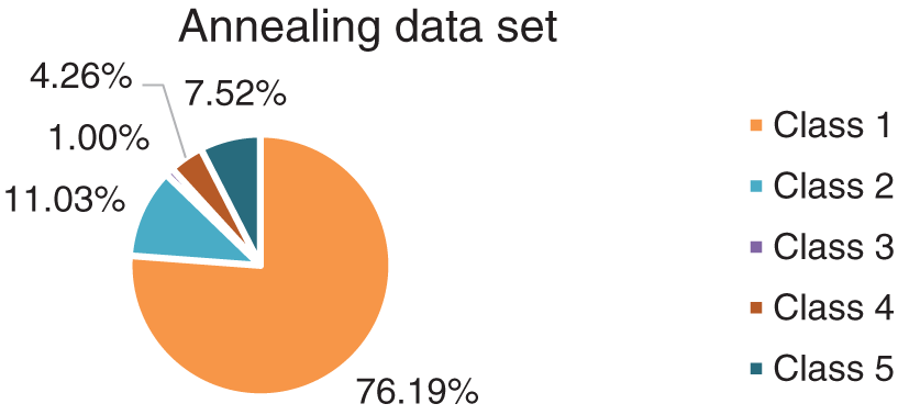
Figure 6: The distribution pie chart of the annealing data set

Tab. 1 lists the multidimensional data, which includes pure numerical data and data comprising numerical and categorical attributes, all of which are within the capacity of the proposed algorithm and broadened application scope of attribute reduction algorithms.

5.2 Analysis of Results

There are 20 outliers in the randomly generated 2-dimensional data set. Given the number of outliers as 20, the objects corresponding to the first 20 largest values of local outlier factor in Eq.(6) are the same as those in Fig. 4b, so the detection accuracy rate is 100%.

For the 8-dimensional data, among the 20 detected outlier objects, only 18 are artificially outliers, and the others are misjudged. The experimental results are not as promising as the 2-dimensional data. In the 16-dimensional data, only 17 of the 20 artificially set objects are identified as outliers, and the others are misjudged. Tab. 2 shows the accuracy of outlier detection of the LOF algorithm on the three randomly generated data sets.

As shown in Tab. 2, the outlier detection accuracy on the randomly 2-dimensional data has the higher value in LOF algorithm than that on the 8-dimensional data or 16-dimensional data. In addition, the 8-dimensional data are better than the 16-dimensional data, revealing that detection accuracy decreases as dimension increases. Data dimension influences the accuracy of the outlier detection algorithm. Therefore, attributes reduction before outlier detection improves the accuracy of outlier detection.

The Wisconsin breast cancer data set comprises 39 presupposed outliers. Among the first 39 objects with the largest local outlier factor calculated by the LOF algorithm, 34 are real outliers, and the other 5 are misjudged dense points. The annealing data set has 190 outliers, of which 72 outliers are real outliers, and the others are misjudged. Tab. 3 shows the accuracy of the algorithm on real data sets.

Four multidimensional data sets (excluding 2-dimensional data) separately underwent data attribute reduction in Algorithm 2. In the process, the attribute subset is determined by calculating neighborhood combinatorial entropy. After attribute reduction, the attribute number of the randomly generated 8-dimensional data is still 8. By comparing the number of attributes, randomly generated 16-dimensional data reduced to 15, and 6 for the Wisconsin breast cancer data set, and 21 for the annealing data set. The variations of their attributes before and after reduction are illustrated in Fig. 7.

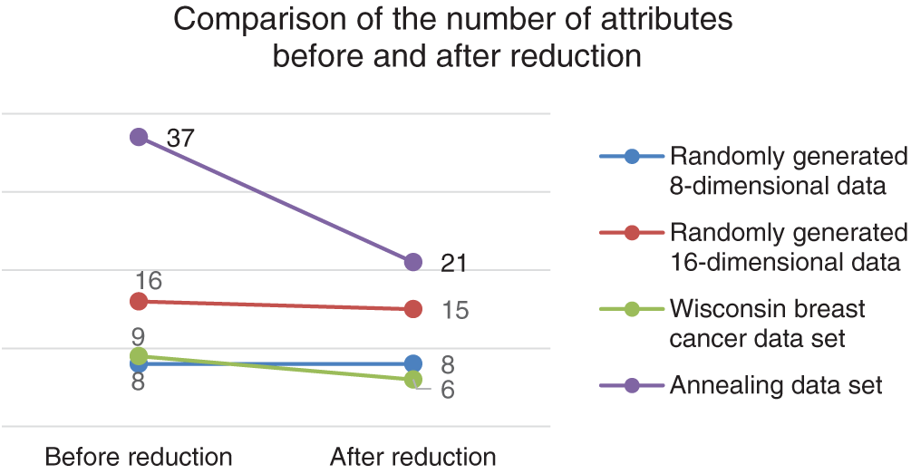
Figure 7: The comparison of the number of attributes before and after reduction analysis of four data sets

From Fig. 7, the system carries out data dimension reduction on data sets, and dimensions of some sets are not reduced, e.g., the 8-dimensional data. By comparing the results of the algorithms, all attributes in a data set have equal influence on the system application (none are filtered out).

Algorithm 1 is adopted to detect outliers from the data sets with reduced attributes. The results are listed in Tab. 4. After attribute reduction, among the top 20 objects with the largest local outlier factors of the 16-dimensional data, 17 are true outliers, and the others are incorrectly judged. The accuracy rate of outlier detection is 85.00%. For the Wisconsin breast cancer data set, after attribute reduction, among the top 39 objects with the largest local outlier factors, 36 are true outliers, and the others are misjudged. The accuracy rate rises to 92.31%. After attribute reduction, for the annealing data set, among the first 190 objects with the largest local outlier factors, 88 are true outliers, and 102 are erroneous. The detection accuracy rate reaches 46.32%. Fig. 8 presents the outlier detection results before and after attribute reduction.

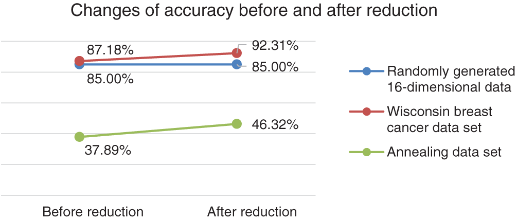
Figure 8: The comparison of outlier detection accuracy before and after reduction in three data sets

As revealed in Fig. 8, attributes identified as useless are reduced by the system, leading to a smaller data size for processing and shortening detection time. For higher outlier detection rate, the attribute reduction algorithm filtered out the error-prone attributes from the system. In addition, enhanced accuracy is obtained in two attribute-reduced data sets, an indication of the validity and effectiveness of the proposed reduction algorithm.

The accuracy of the randomly generated 16-dimensional data remains stable before and after attribute reduction, revealing that the attribute filtering rate is minimal and close to zero, which influences the system. Thus, detection accuracy is intact through attribute reduction.

6  Conclusion

This study combined an attribute reduction algorithm with the LOF algorithm to improve the accuracy of outlier detection for highly dimension numerical and mixed data. Following the algorithms of attribute reduction and the LOF outlier detection, this study analyzed the monotonicity of the attribute reduction algorithm and explained the application of the data processed in outlier detection. We performed the experiments to apply the LOF algorithm on data sets of different dimensions, to assess its performance by calculating its detection accuracy. We also inserted significance determination and attribute reduction algorithms before the LOF algorithm for the five data sets and calculated new detection accuracy. Finally, we compared the feasibility and effectiveness of the two groups of data to assess their detection accuracy before and after data attribute reduction. In comparison, the proposed method reduced data dimensions, calculation time, and improved the outlier detection accuracy when attribute reduction algorithm was combined with outlier detection technology.

Funding Statement: The authors would like to acknowledge the support of Southern Marine Science and Engineering Guangdong Laboratory (Zhuhai) (SML2020SP007). The paper is supported under the National Natural Science Foundation of China (Nos. 61772280 and 62072249).

Conflicts of Interest: The authors declare that they have no conflicts of interest to report regarding the present study.

References

 1.  V. J. Hodge and J. Austin, “A survey of outlier detection methodologies,” Artificial Intelligence Review, vol. 41, no. 3, pp. 85–126, 2004. [Google Scholar]

 2.  C. Cassisi, A. Ferro, R. Giugno, G. Pigola and A. Pulvirenti, “Enhancing density-based clustering: Parameter reduction and outlier detection,” Information Systems, vol. 38, no. 3, pp. 317–330, 2013. [Google Scholar]

 3.  A. F. Oliva, F. M. Pérez, J. V. Berná-Martinez and M. A. Ortega, “Non-deterministic outlier detection method based on the variable precision rough set model,” Computer Systems Science and Engineering, vol. 34, no. 3, pp. 131–144, 2019. [Google Scholar]

 4.  V. Chandola, A. Banerjee and V. Kumar, “Anomaly detection for discrete sequences: A survey,” IEEE Transactions on Knowledge and Data Engineering, vol. 24, no. 5, pp. 823–839, 2012. [Google Scholar]

 5.  J. Jow, Y. Xiao and W. Han, “A survey of intrusion detection systems in smart grid,” International Journal of Sensor Networks, vol. 23, no. 3, pp. 170–186, 2017. [Google Scholar]

 6.  C. Liu, S. Ghosal, Z. Jiang and S. Sarkar, “An unsupervised anomaly detection approach using energy-based spatiotemporal graphical modeling,” Cyber-Physical Systems, vol. 3, no. 4, pp. 66–102, 2017. [Google Scholar]

 7.  S. Fang, L. Huang, Y. Wan, W. Sun and J. Xu, “Outlier detection for water supply data based on joint auto-encoder,” Computers, Materials & Continua, vol. 64, no. 1, pp. 541–555, 2020. [Google Scholar]

 8.  B. Sun, L. Osborne, Y. Xiao and S. Guizani, “Intrusion detection techniques in mobile ad hoc and wireless sensor networks,” IEEE Wireless Communications, vol. 14, no. 5, pp. 56–63, 2007. [Google Scholar]

 9.  S. Hido, Y. Tsuboi, H. Kashima, M. Sugiyama and T. Kanamori, “Statistical outlier detection using direct density ratio estimation,” Knowledge & Information Systems, vol. 26, no. 2, pp. 309–336, 2011. [Google Scholar]

10. M. M. Breunig, H. P. Kriegel, R. T. Ng and J. Sander, “LOF: Identifying density-based local outliers,” in Proc. of the ACM SIGMOD Int. Conf. on Management of Data, New York, NY, USA, pp. 93–104, 2000. [Google Scholar]

11. J. Guan, J. Li and Z. Jiang, “The design and implementation of a multidimensional and hierarchical web anomaly detection system,” Intelligent Automation & Soft Computing, vol. 25, no. 1, pp. 131–141, 2019. [Google Scholar]

12. E. M. Knorr, R. T. Ng and V. Tucakov, “Distanced-based outliers: Algorithms and applications,” VLDB Journal, vol. 8, no. 3, pp. 237–253, 2000. [Google Scholar]

13. A. K. Jain, M. N. Murty and P. J. Flynn, “Data clustering: A review,” ACM Computing Surveys, vol. 31, no. 3, pp. 264–323, 1999. [Google Scholar]

14. F. Jiang, Y. F. Sui and C. G. Cao, “Some issues about outlier detection in rough set theory,” Expert Systems with Applications, vol. 36, no. 3, pp. 4680–4687, 2009. [Google Scholar]

15. B. Liu, Y. Xiao, P. S. Yu, Z. Hao and L. Cao, “An efficient approach for outlier detection with imperfect data labels,” IEEE Transactions on Knowledge and Data Engineering, vol. 26, no. 7, pp. 1602–1616, 2014. [Google Scholar]

16. E. M. Knorr and R. T. Ng, “Algorithms for mining distance-based outliers in large data sets,” in Proc. of the 24rd Int. Conf. on Very Large Data bases, San Francisco, CA, USA, pp. 392–403, 1998. [Google Scholar]

17. J. Tang, Z. Chen, A. W. Fu and D. W. Cheung, “Enhancing effectiveness of outlier detections for low-density patterns,” in Proc. of the 6th Pacific-Asia Conf. Advances in Knowledge Discovery and Data Mining, Taipei, Taiwan, pp. 535–548, 2002. [Google Scholar]

18. K. Zhang, M. Hütter and H. Jin, “A new local distance-based outlier detection approach for scattered real-world data,” in Proc. of the 13th Pacific-Asia Conf. on Advances in Knowledge Discovery and Data Mining, Berlin, Heidelberg, Germany, pp. 813–822, 2009. [Google Scholar]

19. A. Maamar and K. Benahmed, “A hybrid model for anomalies detection in ami system combining k-means clustering and deep neural network,” Computers, Materials & Continua, vol. 60, no. 1, pp. 15–40, 2019. [Google Scholar]

20. F. P. Yang, H. G. Wang, S. X. Dong, J. Y. Niu and Y. H. Ding, “Two stage outliers detection algorithm based on clustering division,” Application Research of Computers, vol. 30, no. 7, pp. 1942–1945, 2013. [Google Scholar]

21. F. Liese and I. Vajda, “On divergences and informations in statistics and information theory,” IEEE Transactions on Information Theory, vol. 52, no. 10, pp. 4394–4412, 2006. [Google Scholar]

22. S. Wu and S. Wang, “Information-theoretic outlier detection for large-scale categorical data,” IEEE Transactions on Knowledge and Data Engineering, vol. 25, no. 3, pp. 589–602, 2013. [Google Scholar]

23. L. N. Wang, C. Feng, Y. J. Ren and J. Y. Xia, “Local outlier detection based on information entropy weighting,” International Journal of Sensor Networks, vol. 30, no. 4, pp. 207–217, 2019. [Google Scholar]

24. P. Maji and P. Garai, “Fuzzy-rough simultaneous attribute selection and feature extraction algorithm,” IEEE Transactions on Cybernetics, vol. 43, no. 4, pp. 1166–1177, 2013. [Google Scholar]

25. Q. H. Hu, D. R. Yu and Z. X. Xie, “Neighborhood rough set based heterogeneous feature subset selection,” Information Sciences, vol. 178, no. 18, pp. 3577–3594, 2008. [Google Scholar]

26. S. U. Kumar and H. H. Inbarani, “PSO-based feature selection and neighborhood rough set-based classification for BCI multiclass motor imagery task,” Neural Computing and Applications, vol. 28, no. 11, pp. 3239–3258, 2016. [Google Scholar]

27. B. Barman and S. Patra, “A novel technique to detect a suboptimal threshold of neighborhood rough sets for hyperspectral band selection,” Soft Computing, vol. 23, no. 12, pp. 1–11, 2019. [Google Scholar]

28. L. Shen and J. H. Chen, “Attribute reduction of variable precision neighborhood rough set based on lower approximate,” Journal of Guizhou University (Natural Sciences), vol. 34, no. 4, pp. 53–58, 2017. [Google Scholar]

29. J. Dai, S. Gao and G. Zheng, “Generalized rough set models determined by multiple neighborhoods generated from a similarity relation,” Soft Computing, vol. 22, no. 7, pp. 2081–2094, 2018. [Google Scholar]

30. J. L. Huang, Q. S. Zhu, L. J. Yang and J. Feng, “A non-parameter outlier detection algorithm based on natural neighbor,” Knowledge-Based Systems, vol. 92, no. 1, pp. 71–77, 2016. [Google Scholar]

31. D. R. Wilson and T. R. Martinez, “Improved heterogeneous distance functions,” Journal of Artificial Intelligence Research, vol. 6, no. 1, pp. 1–34, 1997. [Google Scholar]

This work is licensed under a Creative Commons Attribution 4.0 International License, which permits unrestricted use, distribution, and reproduction in any medium, provided the original work is properly cited.