DOI:10.32604/cmc.2021.018128
| Computers, Materials & Continua DOI:10.32604/cmc.2021.018128 | |
| Article |
Safest Route Detection via Danger Index Calculation and K-Means Clustering
1School of Engineering and Applied Sciences, Bennett University, Greater Noida, India
2Department of ICT Convergence, Soonchunhyang University, Asan, Korea
3Department of Information Systems, Faculty of Computers and Information Sciences, Mansoura University, Mansoura, Egypt
*Corresponding Author: Yunyoung Nam. Email: ynam@sch.ac.kr
Received: 26 February 2021; Accepted: 24 April 2021
Abstract: The study aims to formulate a solution for identifying the safest route between any two inputted Geographical locations. Using the New York City dataset, which provides us with location tagged crime statistics; we are implementing different clustering algorithms and analysed the results comparatively to discover the best-suited one. The results unveil the fact that the K-Means algorithm best suits for our needs and delivered the best results. Moreover, a comparative analysis has been performed among various clustering techniques to obtain best results. we compared all the achieved results and using the conclusions we have developed a user-friendly application to provide safe route to users. The successful implementation would hopefully aid us to curb the ever-increasing crime rates; as it aims to provide the user with a before-hand knowledge of the route they are about to take. A warning that the path is marked high on danger index would convey the basic hint for the user to decide which path to prefer. Thus, addressing a social problem which needs to be eradicated from our modern era.
Keywords: Agglomerative; clustering; crime rate; danger index; DBSCAN
Safe route detection remains a problem which needs to be investigated. An initial approach was implementing video surveillance, which is an important research area in computer vision [1,2]. The most important applications of video surveillance are gait recognition [3,4], action recognition [5,6], object detection [7,8] route safety and name a few more [9,10]. In video surveillance, live reports could be generated, but what if we want our user to get prior knowledge? The need for the solution is well demanded. Though we are in an era where modernization has gained pace, but there is no denial of the fact that heinous crimes as rape exist [11]. All the news and publications stating the statistics and events about the crime activity which shake the very bottom of the heart. The government and police forces are putting in their best, but by far could not reduce this rate. Here, we are making an attempt in the same direction by working on “Safest Route Detection.” Two destinations consist of multiple routes, but a person with no or less knowledge of a place goes for the shortest path, even if it varies just by some kilometers [12]. But what if that path has been consistently registered for crimes? What if by just travelling a few kilometers more, it could prevent a mishap? Even on the public forums as “Crowd form” [13] a demand for such a solution is registered. Google too has taken notice of the problem and has initiated extensive work in a feature called lightning layer [14] which aims at preventing the not so secure routes by pin-pointing the location of the streetlights. The severe need of a counter to this problem has provoked us to investigate further to solve this challenging problem. The primary objective of this work is to develop a system which shows the user that the path they intend to take has been previously reported with crimes and whether it is the safest route between two points or not. The proposed solution gives the users a basic intuition by marking these routes with different danger index so that the user could at least have a hint that the path they intend to choose has been reported with several crimes in the past. Hence allowing them to execute a more rational decision on a route earlier unexplored by them.
To achieve the same, various approaches are explored which align with the proposed problem statement. The problem is relatively much less explored, and the availability of linked resources is constrained. To counter this issue, we have tried to document the results achieved from as many variations as possible and built the primary stage with the best results achieved which not only proves the feasibility of the approach but also instills the idea that a lot more could be done and to counter the steadily increasing problem of crime.
Further, in Section 2 of this article discusses related work; Section 3 gives the details about the Data and method used. In Section 4, the experiment of the proposed schemes is carried out with the results achieved with them. It also discusses the calculation of the Danger Index. Section 5 yields the results of proposed schemes. Ultimately, Section 6 presents the conclusion of the scheme.
The study of crime prevention has been explored at different areas in several community environments [15]. Many researchers have focused on a centralized analysis and research of crime, and these acted as a base and motivated us to work in this domain [16]. However, the calculation of danger index has been too constrained, and the approaches were limited to a single layer of clustering which should not have been the case since both geo-location and the danger index directly affect the clusters built such as Be-safe travel [17]. It uses Google API since that is easily accessible for anyone who would like to drive in a particular region but falls short in knowledge of the routes, which are relatively safer than others from crime. It has prevented three types of crimes such as violence, motor vehicle theft, and theft by weighting. Since this application only focuses on three crimes, one cannot trust it completely as the safe route [18] solution provided by this application might have some dangerous crime records that this application is not considering.
Communities have not let the topic fade away. A research [19] by Washington State Department of Transportation and Mexico City Survey [20], which not only lists the data but also segregates them using Bayes algorithm provides the re-confirmation. A semantically processed dataset with multiple algorithms tested and documented, provides even more insights on the use-case. In SafetiPin [21], a crowd-sourced application, marks the areas as safe and unsafe using pins as the pointers. SafeCity [22], another initiative in the domain is also a crowd-sourced application, which goes a step further and allows users to share the safety tips and self-defense techniques. Even though these applications have been able to achieve excellent results, one major drawback of their application is that of only using the crowd sourced data and not using the criminal data collected by the government. Another approach to tag the danger index is using forecasting [23], i.e., instead of calculation, prediction of the crime stats [24]. “Cluster Boosting Algorithm” [25], which tried to incorporate the factor that dark areas and certain spots are more prone to crime, provides a further direction appreciated by criminologists who understand the importance of local geography. Though documented and appraised, these approaches are far from implementation. Urban navigation [26] an application of the first proposition using crime data from Chicago and Philadelphia, probabilistically estimates the crime but fails to deliver any safe path to the user.
Trippin, which seemed a probable solution, giving the user a danger index insight, to provide the same for all the possible routes, but fails to provid the alternatives to the user. Geographical Information System Based Safe Path Recommender [27], which is a step further and provides the danger index for up to 5 routes, did not take into consideration the fact that each crime is unique and needs to be weighted uniquely. Further, extensive use of API’s made this approach underperform. Another parameter “liveliness index,” i.e., the crowd present, the public amenities, etc. is evaluated by Safely-Reached. A solution totally based on sexual-crime assault [28], which marked the hotspots [29] in the regions, seemed effective but extremely constrained. HumSafar [30], instead of countering the problem, suggested the pooling system in the transport system for more security which at some scope, further increases the crime possibilities. Thus, these models gave us some benchmarks but no workable solution to counter the problem.
While working with geo-location and crime dataset, the data-crunch is a big issue. The dataset used for the proposed work is of New York City taken from online resources NYC Open-Data. It is a well built and updated resource with detailed information revealing no personal data and open for public use. Two datasets, NYPD Arrest Data [31] comprising 1,03,000 rows and 19 columns and Motor Vehicle Collisions-Crashes (https://data.cityofnewyork.us/Public-Safety/Motor-Vehicle-Collisions-Crashes/h9gi-nx95) comprising 1.73 M rows and 29 columns, were studied thoroughly and combined, keeping only the columns that were desired attributes like latitude, longitude, accidents occurred, number of cyclist/motorist/pedestrians injured and killed, crime type comprising categories like dowry deaths, honor killings, exploitation by husband/relatives etc. and dropped columns like arrest key, jurisdiction code, law code and many more which were describing the points directly not linked to the danger index and insignificant in its calculation. The final processed dataset comprised 17,97,784 rows and 16 columns. These rows are down to 80,000 data points, keeping in the consideration the distribution over the New-York city.
3.2 Calculation of Danger Index
Calculation of Danger Index for each Data Point: For each latitude and longitude value, the datasets provided us with the parameters like “Number of Deaths of Cyclists”, “Number of Injured Pedestrians” related to the death and injury of motorcyclists, pedestrians and cyclists in the read accidents. The data additionally provided us with the field, giving the crime description committed at the spot. Though the fields were present, we wanted to club all these fields and complete a column which could present them for a justified representation, the danger index for that geo-coordinate. To achieve this aim, we heeled the approach suggested in [16], where each of the reported deaths was given a value 2 and it marked each of the reported injuries as one. Like so, calculation of the Accident Score for each coordinate utilizing the information from the datasets can be estimated as:
where,
Likewise, for the crime data, we have given each crime a rating to consider its weightage. The reasoning behind doing this is that rape, a far more severe and heinous crime, cannot be considered in the same bucket as chain snatching. Hence, giving the crime score with consideration to severity and passing the weightage to the final danger index. The weightage is presented in Tab. 1.
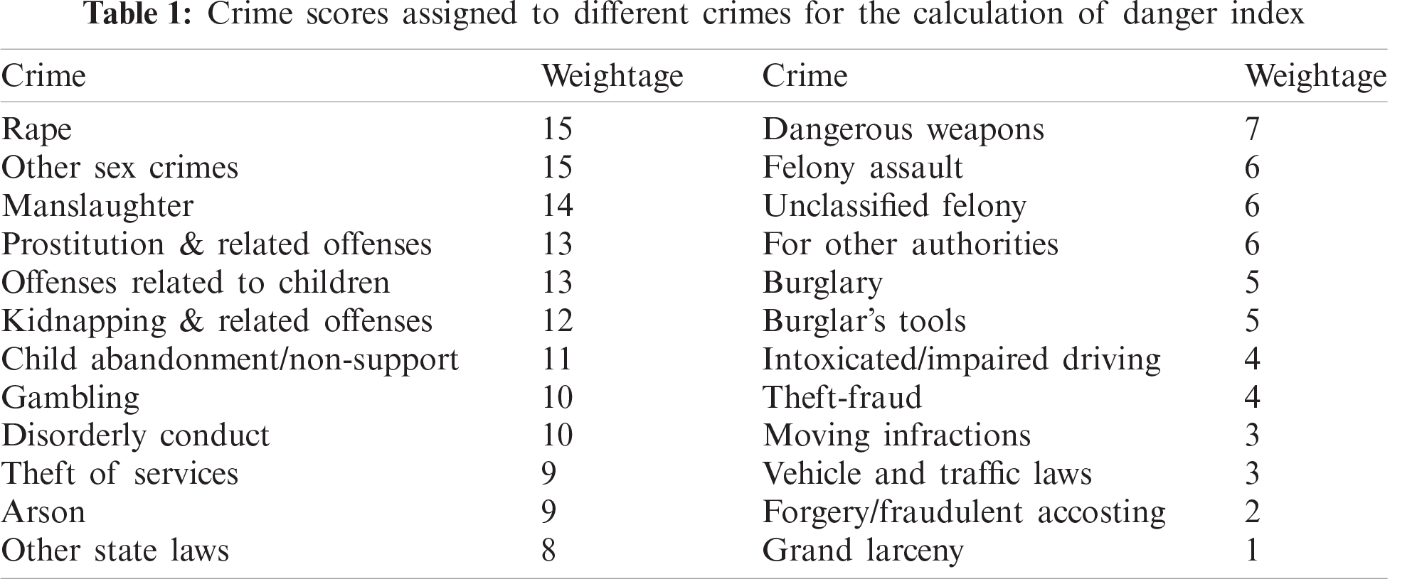
Tab. 1 gives us the crime score (Cs). The Tab. 1 can be further extended depending on the crime category and giving it the appropriate rating. We calculate the resultant danger score using the above two scores. Next we calculate such scores for each of the geo-location lying on the computed route. Conclusively, we normalize this score using the route length (in kilometers), giving us a general score for each path.
For calculation of Crime Score:-
For calculation of Accident Score:-
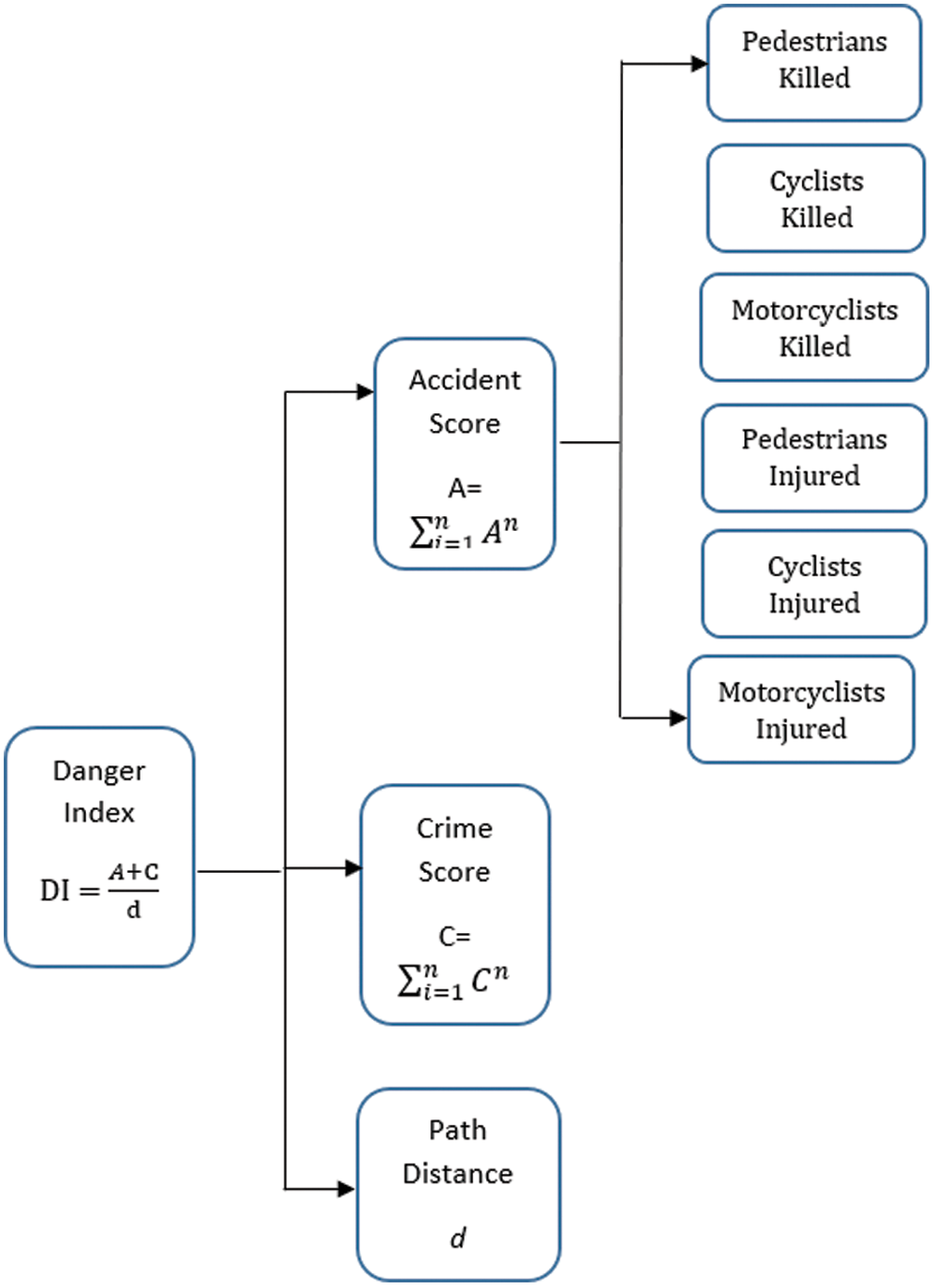
Figure 1: The implementation of danger index and the components involved in the calculation
4.1 Choosing the Optimal Algorithm
Several approaches are available for clustering the data points, but these chiefly depend on the type of dataset we are working upon. The Geo-location dataset does not yield us good results with all the algorithms [32]. From normalization to choosing best optimal technique, such datasets require some prior work to get to know what fits it best. We analyzed the approaches which have shown some optimistic results over these datasets [33].
4.1.1 Hierarchical Clustering (Agglomerate)
This clustering technique, we initially consider all the points in the dataset to be individual clusters. Following each iteration clusters like each other are grouped together until only the required number of K clusters are formed [34].
For a dataset d1, d2, d3 … dn having n elements, we have calculated a distance matrix represented by “dis_mat” using:
where
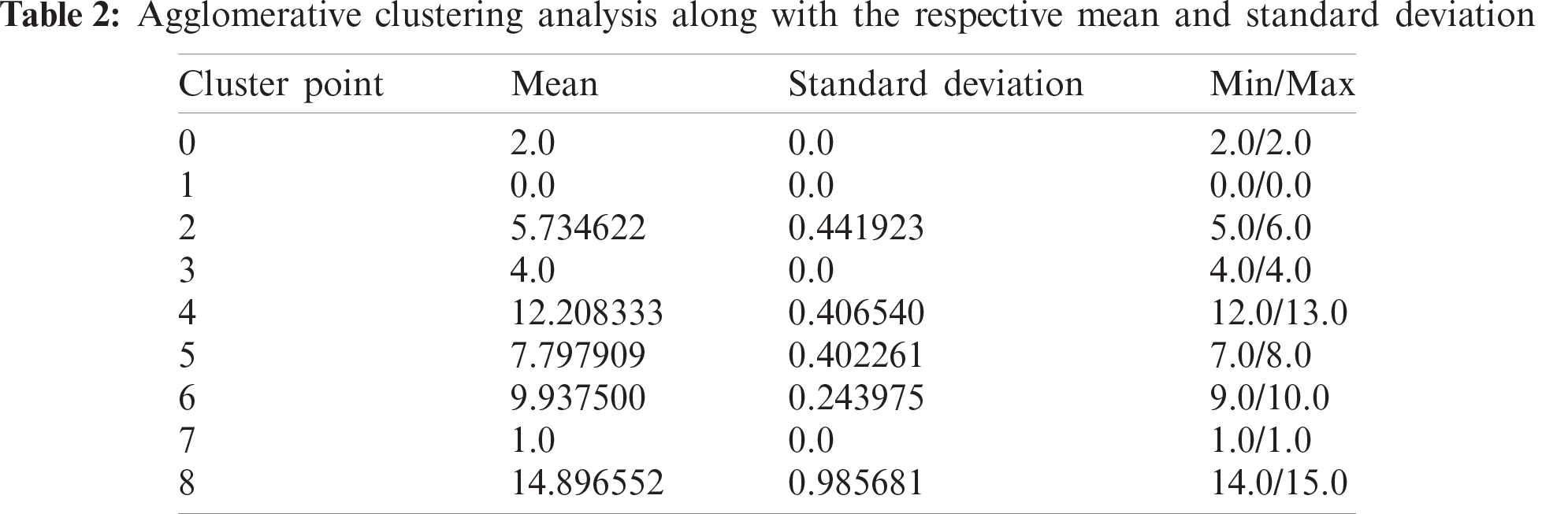
Initially, each data point in the dataset is a “singleton cluster.” We repeat the following process again and again until it leaves us with a single cluster: (1) The clusters gaining the minimum distance to each other are merged. (2) The distance matrix is updated. We demonstrate an example of which in Tab. 2.
It shifts the attention to graph theory where each of the data points is treated as the graph node, making this problem a graph-partitioning problem. The algorithm tries to identify the clusters as the group of nodes judging them based on the edge connecting them.
The Spectral algorithm can be abstracted into the following steps: (1) The data points
The evaluated results are shown in Tab. 3.
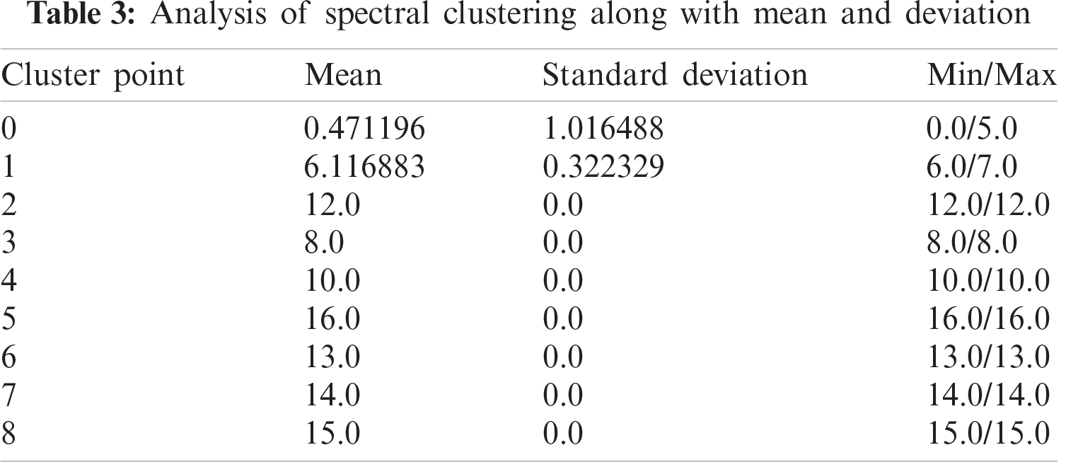
We can discard the spectral clustering on the go as the results on the first sight are not at all representing all the data points. These points vary minimally but drop the high values and show variation in the lower values, which have a more significant number of data-points as compared to high values and should be well segregated. But, seeing Agglomerative Clustering, we cannot directly believe the same. The deviation is not so significant, but it was overruled by the K-means because, as the dataset increases the approach gets more time taking and resource bound, i.e., very high computational complexity and the results are also very poor than the K-means.
An approach, “Density Based Spatial Clustering of Applications with Noise” (DBSCAN), was tried and implemented by determining the clusters [27]. The deviation was not exceptionally high, but the clusters overlapped, making it difficult for the final algorithm to assign a particular cluster to the input geo-coordinate. We can abstract the DBSCAN algorithm into the following steps: (a) Find every point (x1, x2, x3 … xk) present in the dataset; we find the points in the ɛ (eps) neighborhood of respective points. (2) We identify the core points provided; they possess more points than the minimum number of points which are required to specify a dense region. (3) The non-core points are dropped. On the neighborhood graph, determine all the components of core points. (4) For the non-core points, we consider two options: (a) If it lies in the neighborhood of some cluster, that point is assigned to the particular mesh and (b) If no such cluster exists, we assign it to noise. The obtained results achieved from the DBSCAN are shown in Figs. 2a and 2b. Fig. 2a shows overlapping in the resultant clusters which were obtained by using DBSCAN. Fig. 2b shows scattered clusters for the danger indexes of more considerable value as plotted after using DBSCAN for clustering.
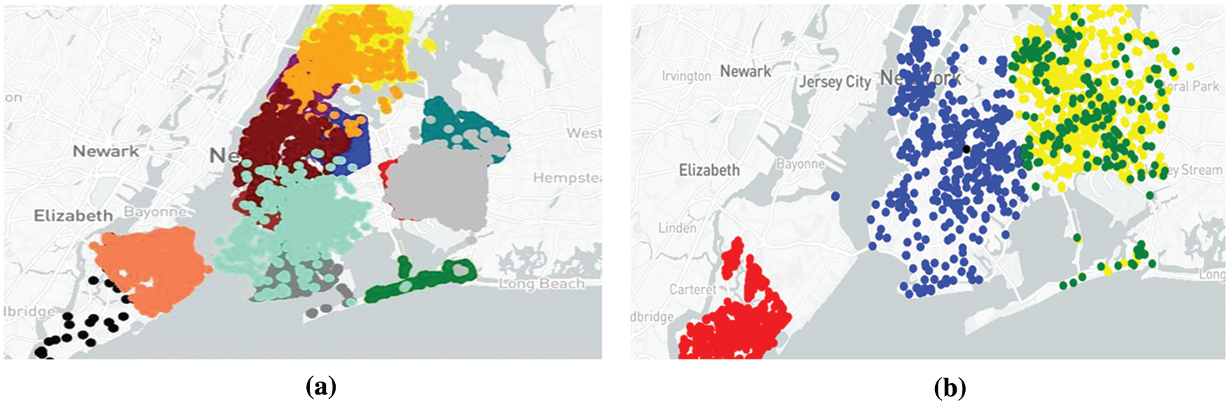
Figure 2: (a) Left-overlapping shown in the resultant clusters which were obtained by using the algorithm: DBSCAN. (b) Right-scattered clusters for the danger indexes of higher value as plotted after using DBSCAN for clustering
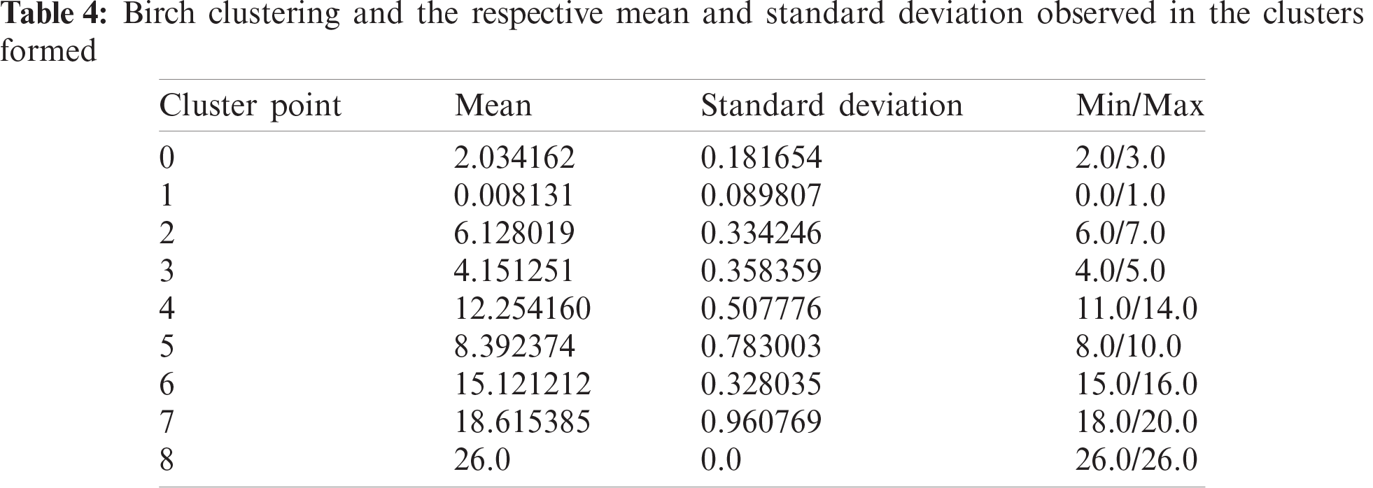
It basically deals with enormous datasets by creating first a compact synopsis comprising as must distribution information which is possible to keep, and then finally it is this summary of data which will be clustered instead of the entire dataset itself. This procedure saves a lot of computation. For Birch clustering [36], we first convert the input of N data points into a tree structure called a “clustering feature (CF)”. It is defined as the set of triplets
The result is a height balanced tree. The further steps include scanning through all the nodes of the CF, building some smaller CF trees for removing any of the outliers present and grouping the nearby sub-clusters into large ones. The distance calculation for two clusters
Another algorithm which showed similar deviation results was birch clustering. The results looked promising at first sight as seen in Tab. 4. But, as we went into the distribution, we found out that the algorithm resulted in a skewed scattering, where the data points were unevenly distributed. With some danger index, the number of data points spiked to 38,361 but for some it was as little as 3. This extreme bias led us to drop this approach for the proposed problem statement.
The algorithm uses distance as the criteria for the grouping of the data points. It originated from signal processing and uses vector quantization which divides the n points into k-clusters and then calculating the distance, assigning the point to the cluster with the nearest mean. The idea behind the K-means clustering is as follows: (1) Choosing the best value for k that fits the proposed work. (2) Initially working with some random centroid here,
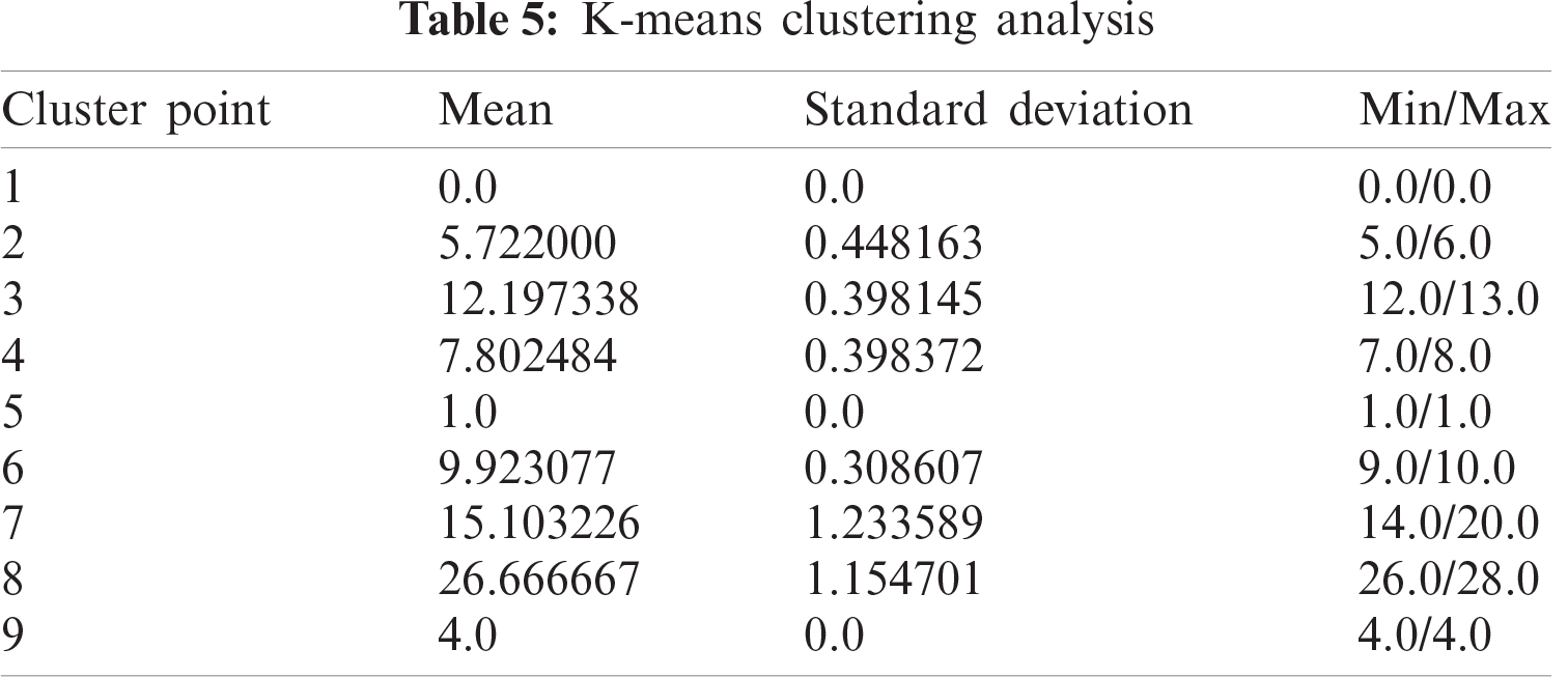
It is concluded that the K-means shows the least deviation for the data points. The variation in the minimum and maximum values is also least, and it gives the representation to the data points very well.
4.2 Choosing the Initial Number of Clusters for the Dataset
After the calculation of danger index, we achieved 19 unique values for this column. We needed to group these values in a way that neither the standard deviation goes too high, nor we have a lot of clusters to deal with. Through experimentation, 10 was the optimal value for the approach. Some results achieved while we list experimentation below in Tabs. 6–8 and the pictorial representation of cluster with k = 10 is shown in Fig. 3.
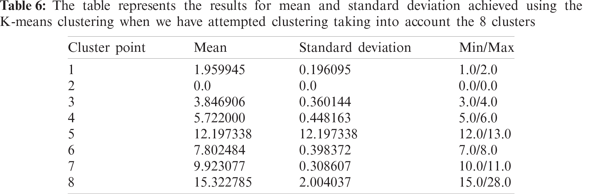
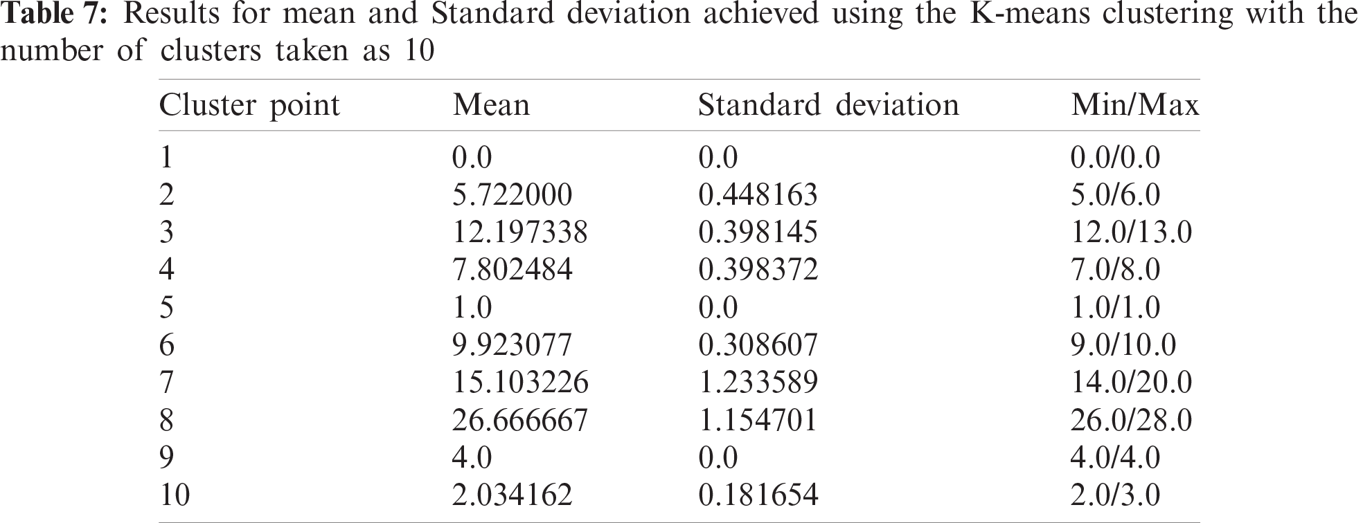
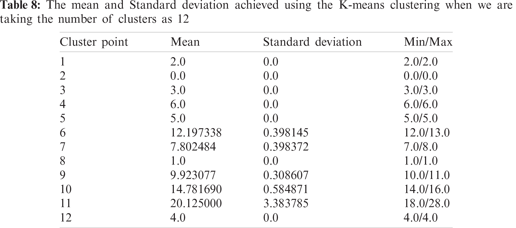
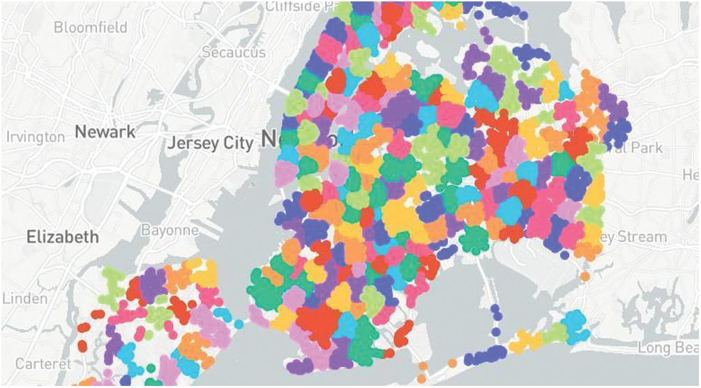
Figure 3: The image represents the clusters achieved as the result of applying K-means on the given coordinates. Each color segment represents a cluster on the basis of the danger index. The number of clusters taken here is 10
The analysis of such results headed us to the conclusion that many clusters set below 10 is not giving the dataset a justified representation and the standard deviation is spiking high. Significantly, if we try to choose a number above 10, we are failing to reduce the standard deviation by any significant term. A greater number of clusters is leading us to having some sets which have very minimum points in them, and this increase in the amount of segmentation is just increasing the computation time with no benefits. Hence, we stick to taking 10 clusters, which is the optimal approach for the proposed work. With an increase in data points or an increase in the number of danger indexes, it is possible that this procedure needs to be repeated to once more find the optimal value for the number of clusters.
4.3 Choosing the Initial Number of Clusters for the Dataset
On calculating the danger index, we receive 10 numbers of unique values of danger index. As the first step, we will cluster the data points based on the danger index. The lesser the number of clusters, the better it will be for the proposed software, but decreasing the number of clusters brings with it the risk of increased standard deviation. Since the problem of finding the safest route has been utmost sensitive to even minor changes in standard deviations, we have needed to find an optimal number. The best way to discover an optimal value is through experimentation.
So, now we have clustered it into 10 clusters. After conducting the first round of clustering we primarily have 10 cluster groups which have a similar danger index value. Presently, in order to make these points useful for us, we have to again cluster them based on the geo coordinates. Each of 10 clusters is separately re-clustered again. Now the number of subclusters in each of the original clusters depends on the number of points in that cluster. Therefore, to generalize it, we choose (number of points in the original cluster) * 0.6 as the number of sub clusters in each of the original clusters. The general approach is (number of points in the original cluster) * 0.5 but the same has not been used because the square root did not generate enough clusters to represent the data distributed over the unified city. Now, the entire sub cluster is associated with 2 feature points-one the geo coordinates of the centroid and second the mean danger index of the subcluster. We create 10 separate lists each for one value of the danger index. Then store all the cluster centroids in them and then dump it to json format. Fig. 4 shows the steps performed before feeding the resultant data to the live deployment.
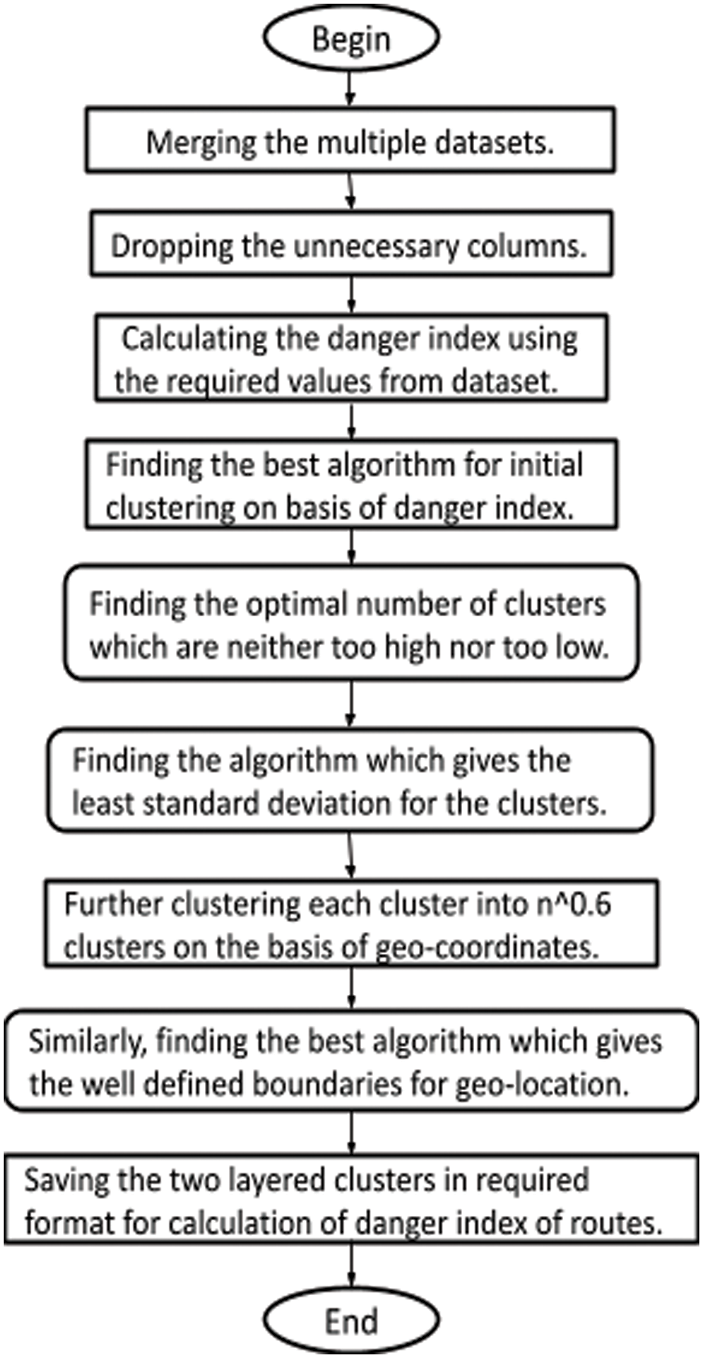
Figure 4: The steps performed before feeding the resultant data to the live deployment
When the user inputs the origin and end destination, using the google maps API, we get all the workable routes between those two points. For each route we calculate its total danger index separately. Let us consider Route 1 that we have got. Now we store all the intermediate latitude and longitude of the routes in a separate list. For each route we consider each latitude longitude pair separately. Promptly for one pair, we compute the closest sub cluster from each of the 10 main clusters. To such a degree, we get several geo-points along with their danger index for each latitude longitude pair from the computed route. Since the danger influence of one point on another point will decrease with increasing distance, we divide the danger index by the distance between the cluster centroid and the original route point. Therefore, each route point now has its own cumulative danger index of these points. Currently, this is performed to all the route points, and they are all added to calculate the final danger index of the route. Now we can return the route, which provides the least danger index.
In our approach, we have implemented clustering at two layers, first based on the Danger Index and the second based on the coordinates to further increase our accuracy and allow routes to be marked more accurately with the danger index. To increase the data, we have taken into far more crime types as compared to any other implementation which gives us an upper hand on the danger index and its presentation of the possibility of occurrence of crime on the route. To grant the user all options, we have tried to show and mark all the routes between any coordinates. Finally, the comparative study helped us prove that our direction for our problem statement is correct.
Thus, through this paper, we are suggesting a probable approach which could work as a base for further development of the full-fledged product which has potentially huge application in the social domain.Through this analysis and research in alternative methods and parameters, we have been able to develop a basic website which uses the Google API to fetch the path coordinates between the inputs of location and individually calculate the danger index for each one giving the user an overview of how safe the path is. The approach employs the data provided by “The NYC Open-Data” consisting of NYPD Arrest Data and Motor Vehicle Collisions-Crashes consisting of highly reliable information with no particulars of individuals. The data is maintained and updated by the City government providing us consistently updated and exhaustive information. The diagram represents the flow of our application is shown in Fig. 5:
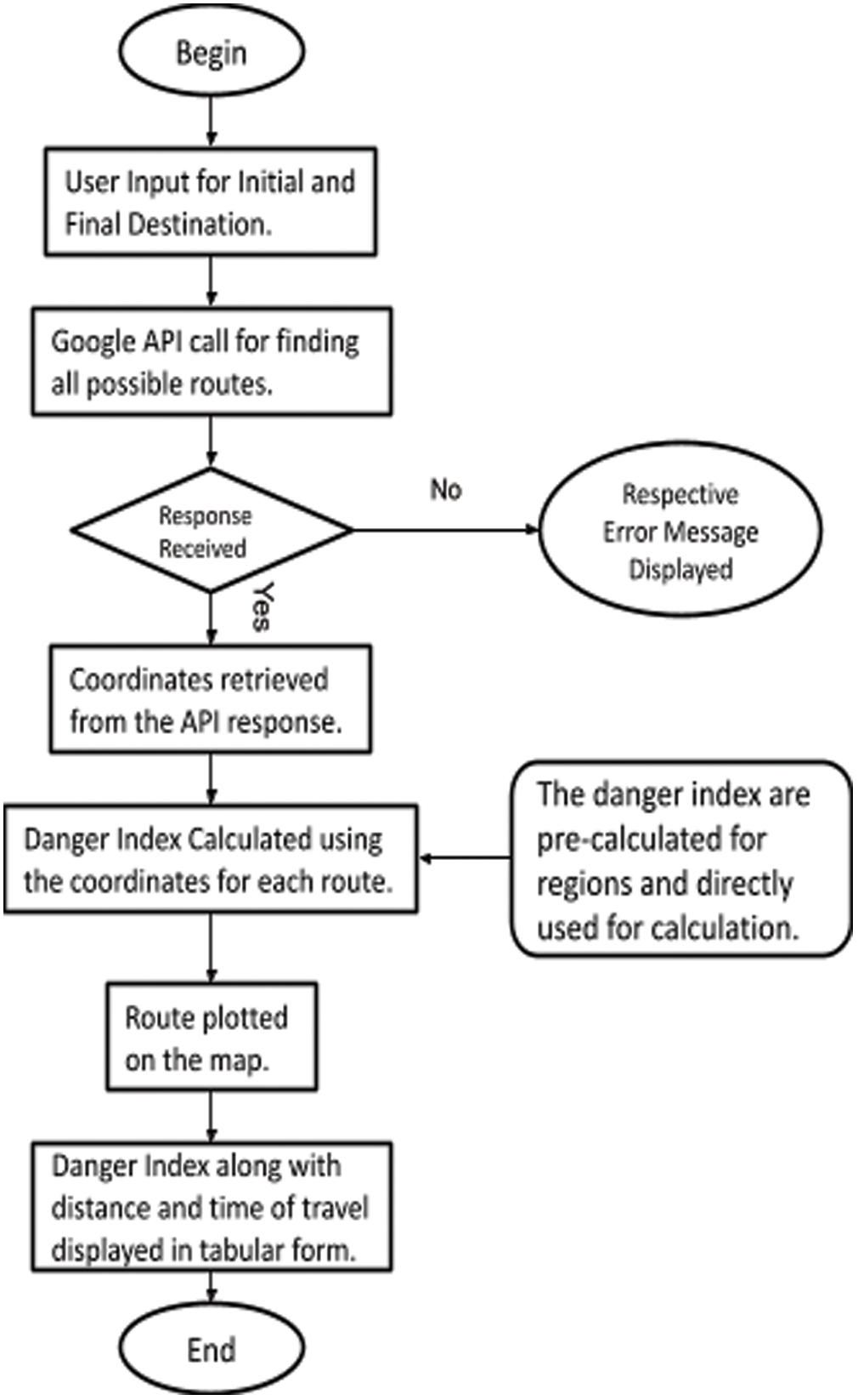
Figure 5: The flow chart for the functioning of the application from the user input until the map is displayed with plotted routes and related information
Fig. 6 shows the multiple paths between the two points, A (here, Central Park, New York, NY, USA) and B (New York State, USA) in the city of New York. These results have been achieved by first clustering the data points in 10 sets regarding the danger index and then according to the latitudes and longitude, resulting in an optimal result for the map of New York city. We focused on K-means as the clusters achieved had a well-defined boundary with least biased distribution and minimal deviation. Each of the routes is represented by a respective colour in the map and has a description related to it, displayed in the tabular format on the live site as represented in Tab. 9.
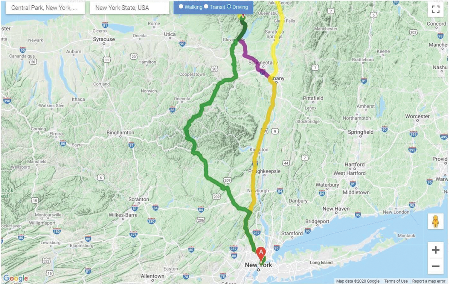
Figure 6: Routes displayed to the user on the web application between the two input locations
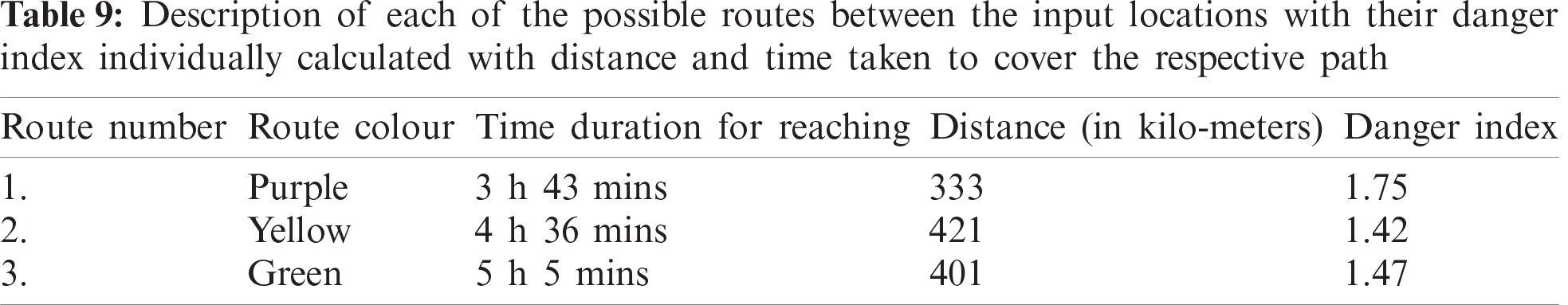
The result displayed comprises the distance, the time duration required to traverse that route and the danger index calculated by the proposed algorithm. Thus, giving the user an overview of the safety on the path, they are about to travel.
We have performed a comparative study between various clustering algorithms and have found out K-means with 10 cluster centres as the most optimal approach, with an average standard deviation of only 0.41232. The number of clusters were varied and compared for getting the best out of them. Also, the different clustering algorithms like Agglomerative Clustering, DBSCAN, Spectral Clustering and so on were taken into consideration and their respective results were listed and compared. A mathematical notation was designed to compute the danger indexed. Extensive experiments reveal that the proposed model can be used for real-time safe route detection.
The approach is not final and can be further extended. The considered factors in our approach are the Crime rate and the accident statistics which could be stretched to the factors like the liveliness of the router, the availability of the streetlights, the availability of the communal facilities as hospitals and so on. If we alter the data set, it will require us to re-verify whether the approach still suits the dataset. Many modifications like the number of clusters, the algorithm used and so on, can be changed and fitted as per the problem statement. An instance could expand our dataset to a unified country instead of merely focusing on a particular city. This would require us to manage a whole current scope of variation in datasets, with the data-points exponentially increased. Hence, we see that there is an immense scope of improvement as the problem directly tries to affect the day-to-day life of the masses. The results presented in the paper help not only one to perceive why K-Means works best but also summarize what other approaches might cause. The K-means additionally allows a scope of improvement, as it has many variations present in the market. More isolated exploration of these variations could yield some more outstanding results. Thus, the variations which are expected and possible are too being assisted and might help in assembling a full-fledged, robust system.
The solution achieved therefore does have its own shortcomings. It is highly based on the input data and if it is altered, a difference in results is expected. More parameters for the calculation of Danger index need to be included in order to make it a fail-proof system. A significant amount of preprocessing is required and the complexity could be further reduced by the use of advanced data structures. Concluding, it is not the ultimate solution but rather a base to construct up a solution which could counter the problem. In near future, the exploration of the used approaches could give some better results. Hence, the variations which are expected and possible are too being assisted and might help in designing a full-fledged, robust system.
Funding Statement: This research was supported by X-mind Corps program of National Research Foundation of Korea (NRF) funded by the Ministry of Science, ICT (No. 2019H1D8A1105622) and the Soonchunhyang University Research Fund.
Conflicts of Interest: The authors declare that they have no conflicts of interest to report regarding the present study.
1. F. Afza, M. Sharif, S. Kadry, G. Manogaran, T. Saba et al., “A framework of human action recognition using length control features fusion and weighted entropy-variances based feature selection,” Image and Vision Computing, vol. 106, pp. 104090, 2021. [Google Scholar]
2. S. Kadry, P. Parwekar, R. Damaševičius, A. Mehmood, J. Khan et al., “Human gait analysis for osteoarthritis prediction: A framework of deep learning and kernel extreme learning machine,” Complex Intelligent Systems, vol. 4, pp. 1–19, 2021. [Google Scholar]
3. H. Arshad, M. I. Sharif, M. Yasmin, J. M. R. Tavares, Y. D. Zhang et al., “A multilevel paradigm for deep convolutional neural network features selection with an application to human gait recognition,” Expert Systems, vol. 8, pp. e12541, 2020. [Google Scholar]
4. A. Mehmood, M. Sharif, S. A. Khan, M. Shaheen, T. Saba et al., “Prosperous human gait recognition: An end-to-end system based on pre-trained CNN features selection,” Multimedia Tools and Applications, vol. 2, pp. 1–21, 2020. [Google Scholar]
5. M. A. Khan, Y.-D. Zhang, S. A. Khan, M. Attique and S. Seo, “A resource conscious human action recognition framework using 26-layered deep convolutional neural network,” Multimedia Tools and Applications, vol. 17, pp. 1–23, 2020. [Google Scholar]
6. K. Javed, S. A. Khan, T. Saba, U. Habib, J. A. Khan et al., “Human action recognition using fusion of multiview and deep features: An application to video surveillance,” Multimedia Tools and Applications, vol. 17, pp. 1–27, 2020. [Google Scholar]
7. M. Rashid, M. Alhaisoni, S.-H. Wang, S. R. Naqvi, A. Rehman et al., “A sustainable deep learning framework for object recognition using multi-layers deep features fusion and selection,” Sustainability, vol. 12, pp. 5037, 2020. [Google Scholar]
8. N. Hussain, M. Sharif, S. A. Khan, A. A. Albesher, T. Saba et al., “A deep neural network and classical features based scheme for objects recognition: An application for machine inspection,” Multimedia Tools and Applications, vol. 9, pp. 1–23, 2020. [Google Scholar]
9. T. Akram, M. Sharif, N. Muhammad, M. Y. Javed and S. R. Naqvi, “Improved strategy for human action recognition; Experiencing a cascaded design,” IET Image Processing, vol. 14, pp. 818–829, 2019. [Google Scholar]
10. M. Sharif, T. Akram, M. Raza, T. Saba and A. Rehman, “Hand-crafted and deep convolutional neural network features fusion and selection strategy: An application to intelligent human action recognition,” Applied Soft Computing, vol. 87, pp. 105986, 2020. [Google Scholar]
11. H. Rong, A. Teixeira and C. G. Soares, “Data mining approach to shipping route characterization and anomaly detection based on AIS data,” Ocean Engineering, vol. 198, no. 2, pp. 106936, 2020. [Google Scholar]
12. C. Ntakolia and D. K. Iakovidis, “A route planning framework for smart wearable assistive navigation systems,” SN Applied Sciences, vol. 3, no. 1, pp. 1–18, 2021. [Google Scholar]
13. R. M. Yas and S. H. Hashem, “A survey on enhancing wire/wireless routing protocol using machine learning algorithms,” in IOP Conf. Series: Materials Science and Engineering, Delhi, India, pp. 12037, 2020. [Google Scholar]
14. G. Gagliardi, M. Lupia, G. Cario, F. Tedesco, F. Cicchello Gaccio et al., “Advanced adaptive street lighting systems for smart cities,” Smart Cities, vol. 3, pp. 1495–1512, 2020. [Google Scholar]
15. D. Fisher, D. Maimon and T. Berenblum, “Examining the crime prevention claims of crime prevention through environmental design on system-trespassing behaviors: A randomized experiment,” Security Journal, vol. 2, pp. 1–23, 2021. [Google Scholar]
16. E. P. Baumer, M. B. Velez and R. Rosenfeld, “Bringing crime trends back into criminology: A critical assessment of the literature and a blueprint for future inquiry,” Annual Review of Criminology, vol. 1, no. 1, pp. 39–61, 2018. [Google Scholar]
17. A. Utamima and A. Djunaidy, “Be-safe travel, a web-based geographic application to explore safe-route in an area,” in AIP Conf. Proc., New Delhi, India, pp. 20023, 2017. [Google Scholar]
18. J. Stilgoe, “Machine learning, social learning and the governance of self-driving cars,” Social Studies of Science, vol. 48, no. 1, pp. 25–56, 2018. [Google Scholar]
19. C. Chaiprasurt, “Decision support system to discover route and time spent at waypoints for cultural tourism and community lifestyles through participation of communities,” in 2019 23rd Int. Computer Science and Engineering Conf., Phuket, Thailand, pp. 129–134, 2019. [Google Scholar]
20. F. Mata, M. Torres-Ruiz, G. Guzmán, R. Quintero, R. Zagal-Flores et al., “A mobile information system based on crowd-sensed and official crime data for finding safe routes: A case study of Mexico City,” Mobile Information Systems, vol. 2016, pp. 1–9, 2016. [Google Scholar]
21. A. B. Haynes, T. G. Weiser, W. R. Berry, S. R. Lipsitz, A.-H. S. Breizat et al., “A surgical safety checklist to reduce morbidity and mortality in a global population,” New England Journal of Medicine, vol. 360, pp. 491–499, 2009. [Google Scholar]
22. P. Rakshita, “Tribal women of India: International and national safeguards---A comparative study,” Commonwealth Law Bulletin, vol. 8, pp. 1–32, 2020. [Google Scholar]
23. C.-H. Yu, W. Ding, P. Chen and M. Morabito, “Crime forecasting using spatio-temporal pattern with ensemble learning,” in Pacific-Asia Conf. on Knowledge Discovery and Data Mining, Tainan, Taiwan, pp. 174–185, 2014. [Google Scholar]
24. Y. Zhang, P. Siriaraya, Y. Kawai and A. Jatowt, “Predicting time and location of future crimes with recommendation methods,” Knowledge-Based Systems, vol. 210, no. 2, pp. 106503, 2020. [Google Scholar]
25. C. P. Haberman and J. H. Ratcliffe, “Testing for temporally differentiated relationships among potentially criminogenic places and census block street robbery counts,” Criminology, vol. 53, no. 3, pp. 457–483, 2015. [Google Scholar]
26. E. Galbrun, K. Pelechrinis and E. Terzi, “Urban navigation beyond shortest route: The case of safe paths,” Information Systems, vol. 57, no. 3, pp. 160–171, 2016. [Google Scholar]
27. Z. Ding, X. Li, C. Jiang and M. Zhou, “Objectives and state-of-the-art of location-based social network recommender systems,” ACM Computing Surveys, vol. 51, no. 1, pp. 1–28, 2018. [Google Scholar]
28. M. E. Ali, S. B. Rishta, L. Ansari, T. Hashem and A. I. Khan, “SafeStreet: Empowering women against street harassment using a privacy-aware location based application,” in Proc. of the Seventh Int. Conf. on Information and Communication Technologies and Development, NY, USA, pp. 1–4, 2015. [Google Scholar]
29. S. Shukla, P. K. Jain, C. R. Babu and R. Pamula, “A multivariate regression model for identifying, analyzing and predicting crimes,” Wireless Personal Communications, vol. 113, no. 4, pp. 2447–2461, 2020. [Google Scholar]
30. M. Arora, N. Kaushik, T. Jain, B. Kaur, P. Vashisth et al., “HumSafar: An android app enabling a safer way to travel,” in 2016 Fourth Int. Conf. on Parallel, Distributed and Grid Computing, Waknaghat, India, pp. 656–661, 2016. [Google Scholar]
31. N. McClain, “Caught inside the black box: Criminalization, opaque technology, and the New York subway MetroCard,” The Information Society, vol. 35, pp. 251–271, 2019. [Google Scholar]
32. F. Amato, F. Guignard, S. Robert and M. Kanevski, “A novel framework for spatio-temporal prediction of environmental data using deep learning,” Scientific Reports, vol. 10, no. 1, pp. 1–11, 2020. [Google Scholar]
33. T. Yorozu, M. Hirano, K. Oka and Y. Tagawa, “Electron spectroscopy studies on magneto-optical media and plastic substrate interface,” IEEE Translation Journal on Magnetics in Japan, vol. 2, no. 8, pp. 740–741, 1987. [Google Scholar]
34. P. J. Kaur, “Cluster quality based performance evaluation of hierarchical clustering method,” in 1st Int. Conf. on Next Generation Computing Technologies, Dehradun, India, pp. 649–653, 2015. [Google Scholar]
35. A. Joshi, A. S. Sabitha and T. Choudhury, “Crime analysis using K-Means clustering,” in 3rd Int. Conf. on Computational Intelligence and Networks, Odisha, India, pp. 33–39, 2017. [Google Scholar]
36. X. Feng and Q. Pan, “The algorithm of deviation measure for cluster models based on the FOCUS framework and BIRCH,” in Second Int. Symp. on Intelligent Information Technology Application, Shanghai, China, pp. 44–49, 2008. [Google Scholar]
 | This work is licensed under a Creative Commons Attribution 4.0 International License, which permits unrestricted use, distribution, and reproduction in any medium, provided the original work is properly cited. |