Computers, Materials & Continua DOI:10.32604/cmc.2021.018670
Article

GPS Vector Tracking Receivers with Rate Detector for Integrity Monitoring

Dah-Jing Jwo* and Ming-Hsuan Lee

Department of Communications, Navigation and Control Engineering, National Taiwan Ocean University, Keelung, 202301, Taiwan
*Corresponding Author: Dah-Jing Jwo. Email: djjwo@mail.ntou.edu.tw
Received: 15 March 2021; Accepted: 16 April 2021

Abstract: In this paper, the integrity monitoring algorithm based on a Kalman filter (KF) based rate detector is employed in the vector tracking loop (VTL) of the Global Positioning System (GPS) receiver. In the VTL approach, the extended Kalman filter (EKF) simultaneously tracks the received signals and estimates the receiver’s position, velocity, etc. In contrast to the scalar tracking loop (STL) that uses the independent parallel tracking loop approach, the VTL technique uses the correlation of each satellite signal and user dynamics and thus reduces the risk of loss lock of signals. Although the VTL scheme provides several important advantages, the failure of tracking in one channel may affect the entire system and lead to loss of lock on all satellites. The integrity monitoring algorithm can be adopted for robustness enhancement. In general, the standard integrity monitoring algorithm can timely detect the step type erroneous signals. However, in the presence of ramp type slowly growing erroneous signals, detection of such type of error takes much more time since the error cannot be detected until the cumulative exceeds the specified threshold. The integrity monitoring based on the rate detector possesses good potential for resolving such problem. The test statistic based on the pseudorange residual in association with the EKF is applied for determination of whether the test statistic exceeds the allowable threshold values. The fault detection and exclusion (FDE) mechanism can then be employed to exclude the hazardous erroneous signals for the abnormal satellites to assure normal operation of GPS receivers. Feasibility of the integrity monitoring algorithm based on the EKF based rate detector will be demonstrated. Performance assessment and evaluation will be presented.

Keywords: Global positioning system; vector tracking loop; integrity monitoring; rate detector; slowly growing errors

1  Introduction

The Global positioning system (GPS) [1–3] receiver generally accomplishes two major functions, i.e., signal tracking and navigation processing. The signal tracking intends to adjust the local signal to synchronize the local code phase with the received satellite signal. Traditional GPS receivers track signals from different satellites independently. Each tracking channel measures the pseudorange and pseudorange rate, respectively, and then sends the measurements to the navigation processor, which solves for the user’s position, velocity, clock bias and clock drift (PVT).

The traditional scalar tracking loop (STL) processes signals from each satellite separately. It is more like an open loop system and provides degraded performance when scintillation, interference, or signal outages occur. The vector tracking loop (VTL) [4–11] provides a deep level of integration between signal tracking and navigation solutions in a GPS receiver and results in several important improvements over the traditional STL. The most notable advantage of the VTL is the increased interference immunity, and there are some other benefits, such as robust dynamic performance, the ability to operate at low signal power and bridge short signal outages. Although the VTL architectures provide several important advantages, they suffer some fundamental drawbacks. The errors in navigation solutions may degrade the accuracy of the tracking loop results. The most significant drawback is that failure of tracking in one channel may affect the entire system and lead to loss of lock on all satellites. To ensure a user position solution with predetermined uncertainty levels, reliability monitoring and assessment are essential.

Navigation system performance can be classified as four major aspects by the Federal Aviation Administration (FAA): accuracy, integrity, continuity, and availability. Integrity is a measure of the trust that can be placed in the correctness of the information supplied by the total system. This includes the ability of a system to provide timely and valid warnings to the user when the system must not be used for the intended operation. Reliability monitoring typically consists of testing the residuals of the observations statistically on an epoch-by-epoch basis with the aim of detecting and excluding measurement errors and, therefore, obtaining consistency among the observations with assigned uncertainty levels. The receiver autonomous integrity monitoring (RAIM) [12–19] research began in the 1980s. The principle is the use of redundant satellite observations (redundant message) by mutual checking data consistency (consistency check). It does detect of whether the satellite signals to provide the correct information. The theoretical basis is statistical assumptions test that randomly distribution applicable for Chi-square distributed. Classical RAIM techniques aiming at fault isolation lead to a computationally intensive user-level integrity monitoring process when multiple faults are considered.

In general, the standard integrity monitoring algorithm can timely detect the step type erroneous signals. In the presence of slowly growing ramp type erroneous signals, however, detection of such type of error requires much more time since the error cannot be detected until the cumulative exceeds the specified threshold. The rate detector is realized using a simple Kalman filter (KF) for monitoring the slowly growing erroneous signals. The test statistic of pseudorange residual of rate detection in association with the extended Kalman filter (EKF) [20] is applied to calculate the variance ratio of test statistic for determination of whether the ratio exceeds the allowable values.

This paper employs the integrity monitoring algorithm based on the rate detection approach to the GPS VTL for robustness improvement in the presence of slowly growing ramp type erroneous signals. The remainder of this paper is organized as follows. Preliminary background on GPS navigation filter in vector tracking configuration with integrity monitoring is reviewed in Section 2. In Section 3, the integrity monitoring algorithms are briefly reviewed, including RAIM and the Autonomous Integrity Monitored Extrapolation (AIME). The Kalman filter based rate detector is introduced in Section 4. In Section 3, illustrative examples are presented to evaluation of the effectiveness of the proposed algorithm. Conclusions are given in Section 6.

2  GPS Receiver Vector Tracking with Integrity Monitoring

The carrier and code tracking loops play a key role in a GPS receiver. Specifically, a delay lock loop (DLL) is used to track the code phase of the incoming pseudorandom code and a carrier tracking loop, such as a frequency lock loop (FLL) or a phase lock loop (PLL), is used to track the carrier frequency or phase. Traditional GPS receivers have some parallel DLLs. Each loop tracks a satellite to estimate the corresponding pseudorange. The parallel pseudorange measurements are sent to the navigation filter, where the navigation state was calculated.

The drawback of STL is that it neglects the inherent relationship between the navigation solutions and the tracking loop status. A STL is more like an open loop system and provides poor performance when scintillation, interference, or signal outages occur. The VTL provides a deep level of integration between signal tracking and navigation solutions in a GPS receiver and results in several important improvements over the traditional STL such as increased interference immunity, robust dynamic performance, and the ability to operate at low signal power and bridge short signal outages. The VTL differs from the traditional STL in that the task of navigation solutions, code tracking and carrier tracking loops for all satellites are combined into one loop. The center part of a VTL is the EKF which provides an optimal estimation of signal parameters for all satellites in view and user PVT solutions based on both current and previous measurements from all satellites.

In the VDLL, each channel does not form a loop independently. The vector comprised of outputs of all the code phase discriminators is the measurement of navigation filter. The navigation state is estimated by navigation filter, and the error signals arise from the estimated user positions and the satellite positions calculated by the ephemeris. That is to say, the code loop Numerically Controlled Oscillator (NCO) in SDLL is replaced by the estimated user positions, to control the update of the local code. When one channel experiences interference or signal outages in the VTL, the information from other satellites can be used estimate the status of this channel. The EKF is employed to estimate the PVT of the receiver.

The architecture of the VTL can be different depending on its implementation. The tracking input is not directly connected to the tracking control input rather the discriminator output is used in estimating pseudoranges. The EKF in turn predicts the code phases. In VTL all channels are processed together in one processor which is typically an EKF. Therefore, even if the signals from some satellites are very weak the receiver can track them from the navigation results of the other satellite. VTL is a very attractive technique as it can provide tracking capability in degraded signal environment. Fig. 1 shows the signal tracking configurations for scalar tracking loop and vector tracking loop, respectively, of the GPS receivers.

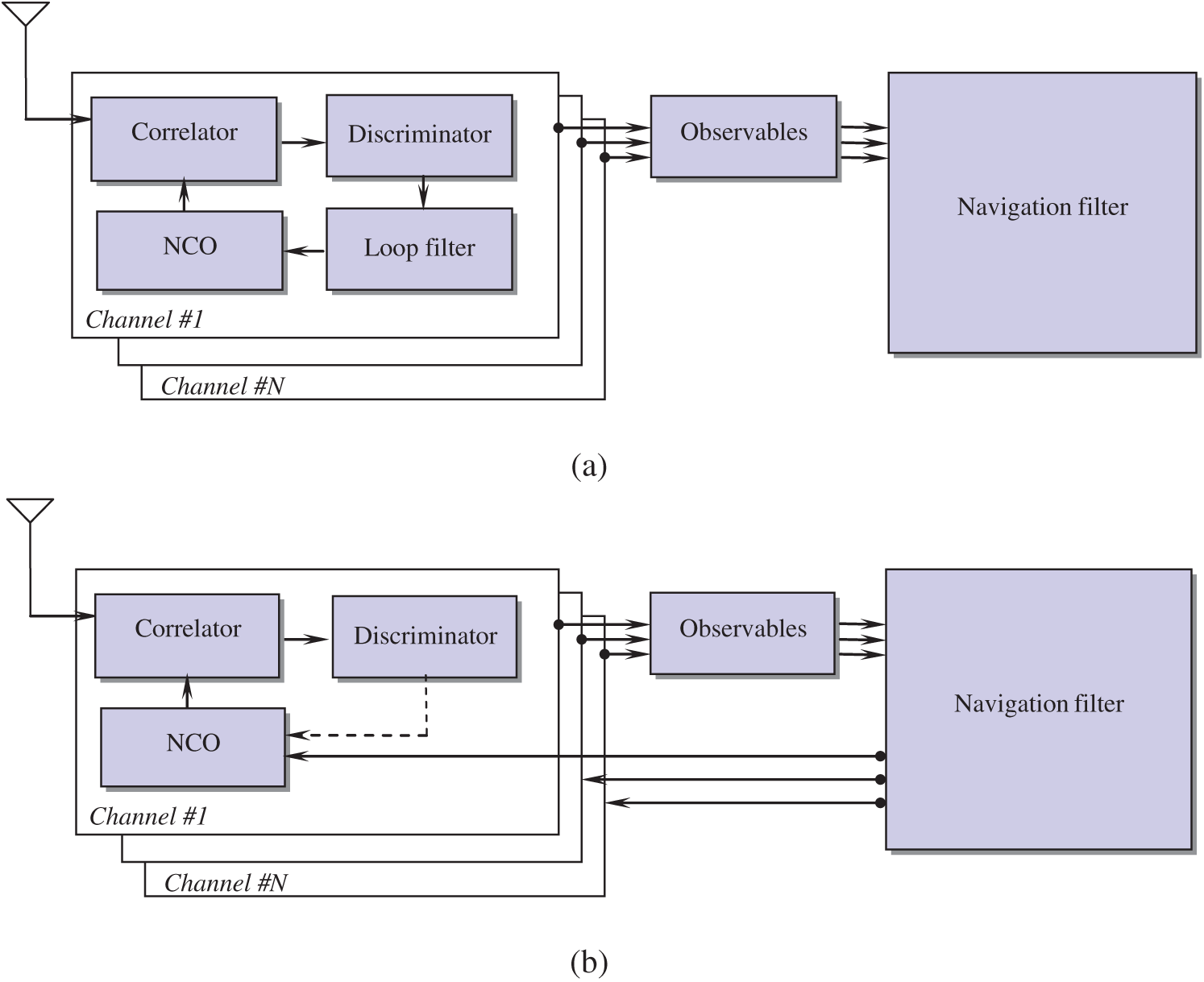
Figure 1: The signal tracking configurations for the global positioning system (GPS): (a) scalar tracking loop; (b) vector tracking loop

The conventional VTL based on the discriminator consists of correlator, discriminator and NCO. The loop filter ca be removed in each channel. The VTL discriminator outputs of each channel are used as the measurement of the navigation extended Kalman filter. The Doppler frequency and the pseudoranges are calculated from the estimated user position and velocity of the navigation filter. In general, it is known that the VTL based on the discriminator provides users an accurate position and Doppler frequency than the scalar vector tracking loop. The VTL based on the discriminator does not possess sufficient capability to deal with several problems, such as a rejection of channel with a low quality signal, high dynamic situation and others.

3  Integrity Monitoring Algorithms

Navigation system integrity refers to the ability of the system to provide timely warming to users when the system should not be used for navigation. It is regarded as a risk factor to provide timely warning to users when the position error exceeds a specified limit. In short, the altering system with integrity is heuristic in time to alarm when the position error over the value of a threshold. Thus the system is said to possess the function of “integrity.”

3.1 Receiver Autonomous Integrity Monitoring

The performance and availability (i.e., the existence of the conditions for failure detection) of the RAIM have been shown to be a function of a number of factors, such as the number of redundant observations available, the geometry of the available satellites, the probability with which an error must be detected, the size of acceptable error, and the quality of the observations used.

A variety of RAIM schemes have been proposed, all of which are based on some kind of self-consistency check among the available redundant measurements. Basically, the RAIM algorithms are classified into two groups, snapshot (utilizing only the measurements at the current epoch) and sequential (utilizing both current and historical measurements).

The conventional RAIM scheme belongs to the type of “snapshot” approaches, which assume each measurement is uncorrelated from one minute to the next time. With this method, only current redundant measurements are used in the self-consistency check. The instantaneous “snapshot” least squares residual vector is used to compute the test statistic. The other method is the sequential algorithm that uses the Kalman filter. Several typical snapshot and sequential algorithms will be first reviewed for gaining some more insight on the RAIM algorithms.

In addition to the least square method, the EKF can be used for navigation solution or RAIM processing. It is a recursive filter, for which there is no need to store past measurements for the purpose of computing present estimates. Given a signal that consists of a linear dynamical system driven by stochastic white noise processes, the EKF provides a method for constructing an optimal estimate of the system state vector.

Three RAIM methods have received special attention on GPS integrity. These include: (a) Range comparison method; (b) Least squares residual method; (c) Parity method. All three methods are snapshot schemes in that they assume that noisy redundant range-type measurements are available at a given sample point in time.

Linearization of the pseudorange equation of GPS is

y=Hx+e (1)

This equation can be solved using the least squares approach

x^LS=(HTH)−1HTy (2)

The least squares residuals method is based on the solution of least squares method, we have

y^=Hx^LS=H(HTH)−1HTy (3)

The n×1 vector

w=y−y^=[I−H(HTH)−1]y (4)

Based on this vector, the satellite failure can be detected based on the sum of squared errors (SSE)

SSE=wTw (5)

The RAIM is said to be available if at least five satellite measurements are available in the required geometric configuration.

The EKF generally uses linear approximation over the smaller ranges of state space. In something akin to a Taylor series, we can linearized the estimation around the current estimates. Assuming that the dynamic process model has a state vector x, we can write nonlinear dynamic process model and measurement model as fallows

xk+1=f(xk,k)+wk,wk∼N(0, Qk) (6)

zk=h(Xk,k)+vk,vk∼N(0, Rk) (7)

where the random variables wk and vk represent the process and measurement white noise sequences; the nonlinear function f relates the state at previous time step k−1 to the state at the current time step k. The nonlinear function h relates the state xk to the measurement zk. Since the measurement model is nonlinear, the EKF is employed for navigation processing.

As for the sequential approach of RAIM, the commonly used EKF is summarized as follows:

Kalman gain:

Kk=Pk−HkT[HkPk−HkT+Rk]−1 (8)

Update the estimation:

x^k=x^k−+Kk[zk−h(x^k−)] (9)

Update the error covariance matrix:

Pk=[I−KkHk]Pk− (10)

Predict state of reference error:

x^k+1−=Φkx^k (11)

Estimate the error covariance matrix:

Pk+1−=Φk+1PkΦkT+Qk (12)

where Φk is the state transition matrix.

The state vector is composed of position errors, velocity errors, in the east, north and altitude component, clock bias and drift. The state equation is linear represented by the form

xk+1=Φkxk+wk (13)

with the state vector

where

Consider the user position in three dimensions, denoted by (xu,yu,zu), the GPS pseudorange observables made to the i-th satellite can then be written as

ρi=(xi−xu)2+(yi−yu)2+(zi−zu)2+ctb+vρi (14)

where (xi,yi,zi) denotes the i-th satellite’s position in three dimensions, i=1,…,n; c is the speed of light; tb is the receiver clock offset from system time; and vρi is the pseudorange noise.

The measurement equations of the navigation RKF is given by:

zk=hk(xk)+vk=[ρk1⋯ρkiρ˙k1⋯ρ˙ki]T (15)

and

where the direction cosines (hx,i,hy,i,hz,i) are given by:

The system architecture of the vector tracking loop with RAIM employed is shown as in Fig. 2.

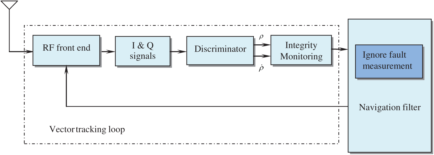
Figure 2: The system architecture of the vector tracking loop with RAIM

3.2 Autonomous Integrity Monitored Extrapolation

As a type of sequential approach, the AIME was proposed by Diesel et al. [16]. It is a software mechanization for integrating GPS with INS to solve the GPS integrity/availability problem. Using Kalman filter principles, AIME generates a least-squares solution both the present position output and detection and isolation of failure based on the entire past history of measurements.

The residuals of extended Kalman filter defined as

υk=zk−z^k− (16)

has zero mean, E[υk]=0 and covariance

E[υkυkT]=Uk=HkPk(−)HkT+Rk (17)

where the predicted measurement z^k−=h(x^k−,k).

Satellite failures are detected by using the magnitude of the normalized residual vector s as the test statistic:

λk=s2=sTs=υkTUk−1υk (18)

The AIME approach utilizes the statistic s2 (sum squared residual, or simply SSR for short) to detect failure, in the way that the parity vector squared magnitude p2 is used in RAIM. If there are n satellites in view, s2 is Chi-square distributed with n degrees of freedom, and p2 is Chi-square distributed with n − 4 degrees of freedom. This means that AIME can detect failures with as few satellites in view, while RAIM requires a minimum of five satellites with good geometry. The significant difference is that s2 depends on the entire past history of measurements.

The innovation property enables it to detect slow satellite drifts. This is done by estimating the mean of the residuals over a long time interval, to determine the averaged residual. Satellite failures are detected by using the magnitude of the normalized residual vector s as the test statistic:

The averaged inverse covariance and averaged residual is obtained as:

υavg=(Uavg−1)−1Uavg−1υk (19)

and

savg2=υavgTUavg−1υavg (20)

In the process of failure detection, the threshold sD for detecting failures is Chi-square distributed with n degrees of freedom. It is selected to result in the false alarm rate. The probability density function (pdf) associated with a Chi-square distribution with k degrees of freedom is

f(x)={2−k/2Γ(n/2)x(k/2)−1e−k/2if x>00if x≤0 (21)

where Γ(x)=∫0∞tx−1e−tdt indicates the gamma function.

The fault alarm rate (denoted as PFA) equation is defined as

∫a∞f(x)dx=PFA (22)

The parameter a is the normalized threshold for |s2| as the test statistic. Therefore the normalized threshold for |s| as the test statistic is a. The threshold sD=σ⋅a, where σ is the standard deviation. When s≥sD, a “failure alarm” is reported; on the other hand, when s<sD, the GPS receiver is in normal condition, and no failure is reported.

4  Kalman Filter Based Rate Detector

The ramp type failures are more difficult to detect. It is time consuming to detect if the rate of growth is lower (e.g., 2 m/s or less for a satellite range). The algorithm, referred to as the rate detector algorithm [18,19], is effective for slowly growing erroneous signals. The rate detector algorithm is based on the concept of detection of the rate of the test statistic. The test statistic is formed by using the innovation of the main navigation EKF and covariance matrix of the innovation. It was proposed in the AIME method that averages of the innovation and its covariance matrix are to be used.

As for the rate detector algorithm, the test statistic is formed by instantaneous values of the innovation and its covariance matrix since the averaging process is no longer required due to the fact that the rate is estimated directly from the signal. To detect the rate of a signal, a Kalman filter can be utilized. The test statistic acts as an input signal to a simple Kalman filter configuration. This has the advantage that noise in the signal can be accounted for in the noise matrices of the filter. The Kalman filter is adopted so that the test statistic and its rate of change, i.e., its velocity, can be estimated, where the velocity is one of the states of the Kalman filter. An alert is generated when this velocity state exceeds the calculated threshold. A high level configuration of the rate detector algorithm is shown in Fig. 3.

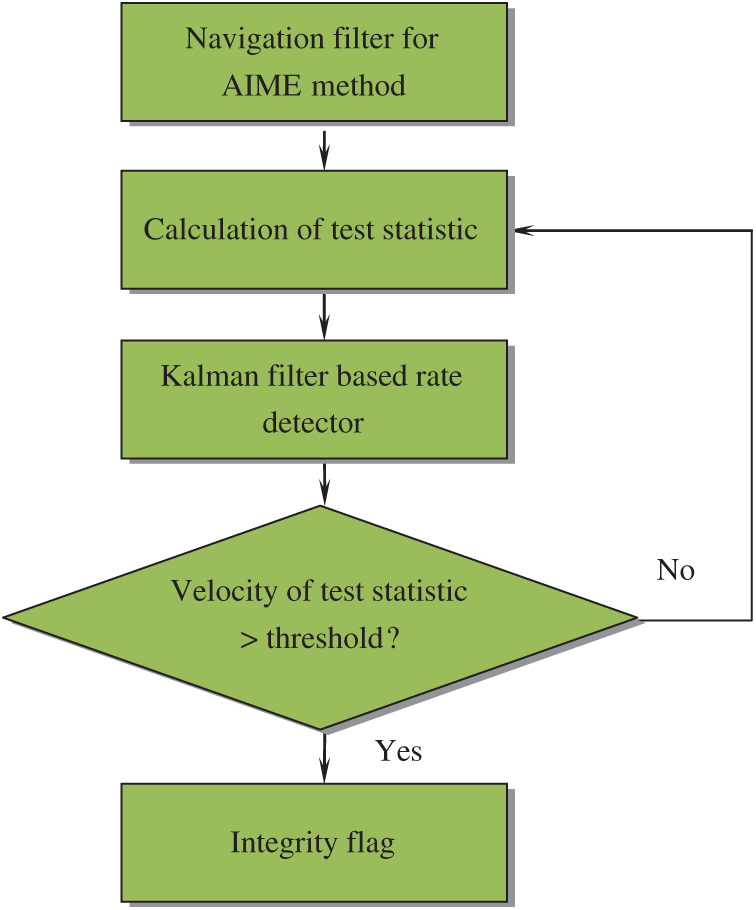
Figure 3: The high level configuration of the rate detector algorithm

To tackle the problem associated with the noise of the estimated velocity, a Kalman filter is formulated. There are three states involved, i.e., x=[pva]T=[λkλ˙kλ¨k]T. The test statistic is assumed underlying velocity model is of the form:

v˙=−αv(t)+a(t)+ξ (23)

The process model then takes the form:

[p˙v˙a˙]=[0100−α1000][pva]+[u1u2u3] (24)

where α is a constant whose value can be adjusted according to the magnitude of noise in the system, and a is the new state added that represents the acceleration of the signal. The value of the covariance noise matrix for the dynamic model is dependent on the selection of the correlation constant α. The measurement matrix Hk is [100]. In order to calculate the test statistic, it is taken out of its rate of estimated state which is expressed as follows:

Vrate=C⋅[pva] (25)

where C=[010].

The test statistic (D) for the rate detector can be defined as:

D=|Vrate|σ0PV (26)

where σ0 represents the standard deviation of Vrate, PV represents the variance of rate state derived by the Kalman filter, and thus D∼N(0,1). If there are n satellites, each of them has the same false alarm. For all satellites of false alarm is Pfa, so its single is Pfa/n. We can get the velocity detection threshold which is based on false alarm. The probability of false alert for the velocity state is given by:

Pfan=P(D≥vD)=12π∫vD∞e−x22σ2dx (27)

vD represents the threshold. When a failure occurs, the test statistic D will exceed the threshold.

The innovation and its covariance obtained from the EKF are employed to form the measurement of the KF based rate detector. This measurement is in fact the test statistic defined by the AIME method. This is used by the Kalman filter for the rate detector algorithm as its measurement. The rate detector algorithm estimates the velocity of this measurement and compares it with velocity threshold to set or reset the status of the integrity flag. Fig. 4 provides the information flow of the algorithm involving the navigation EKF with the Kalman filter based rate detector for monitoring the test statistic by the AIME.

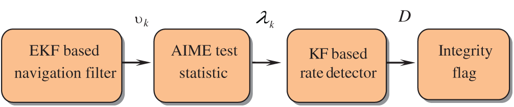
Figure 4: Information flow of the algorithm involving the extended Kalman filter (EKF) based navigation filter and Kalman filter (KF) based rate detector

5  Illustrative Examples

Simulation experiments have been carried out for confirmation of the effectiveness and justification of the performance for the proposed configuration. Simulation was implemented on a personal computer with the computer codes developed by the authors using the Matlab® software. The commercial software Satellite Navigation (SatNav) Toolbox [21] was employed for generating the satellite positions and pseudoranges. Furthermore, the Inertial Navigation System (INS) Toolbox [22] was employed for generating the simulated vehicle trajectory. A simulated vehicle trajectory originating from the position of North 25.1492 degrees and East 121.7775 degrees at an altitude of 100m was assumed. The location of the origin is defined as the (0, 0, 0) m location in the local tangent East-North-Up (ENU) frame. The test trajectory and the satellites in view for the simulation are shown in Fig. 5.

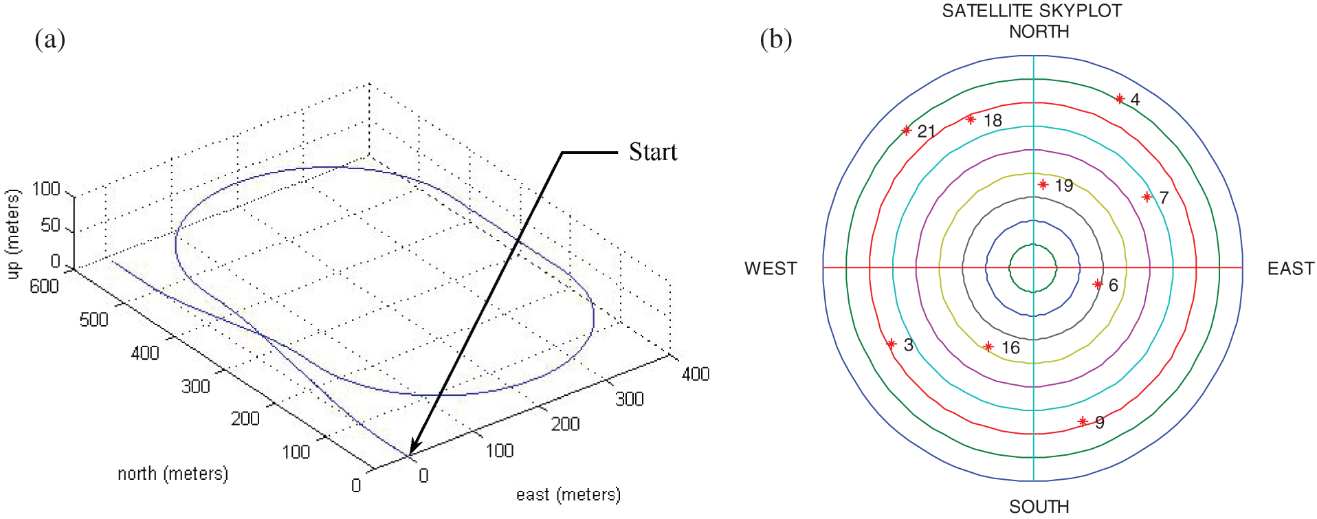
Figure 5: The (a) vehicle trajectory and (b) skyplot in simulation

The experiments cover two parts dealing with two types of erroneous signals. The first part deals with performance test for the step type erroneous signals; the second part deals with the tests for slowly growing ramp type erroneous signals. Performance of the integrity monitoring for the rate detector algorithm as compared to the conventional approach is presented.

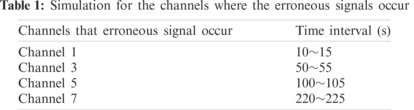
(1) Scenario 1: test for step type erroneous signals

To validate the performance of integrity monitoring for the vector tracking configuration of GPS for the step type erroneous signals, a 100 meters error is added into four satellite channels (i.e., 1, 3, 5, 7, respectively) lasting for 5 s at each time interval, shown as in Tab. 1. The east, north and vertical errors are shown in Fig. 6. Fig. 7 shows the time history data of test statistic for Scenario 1.

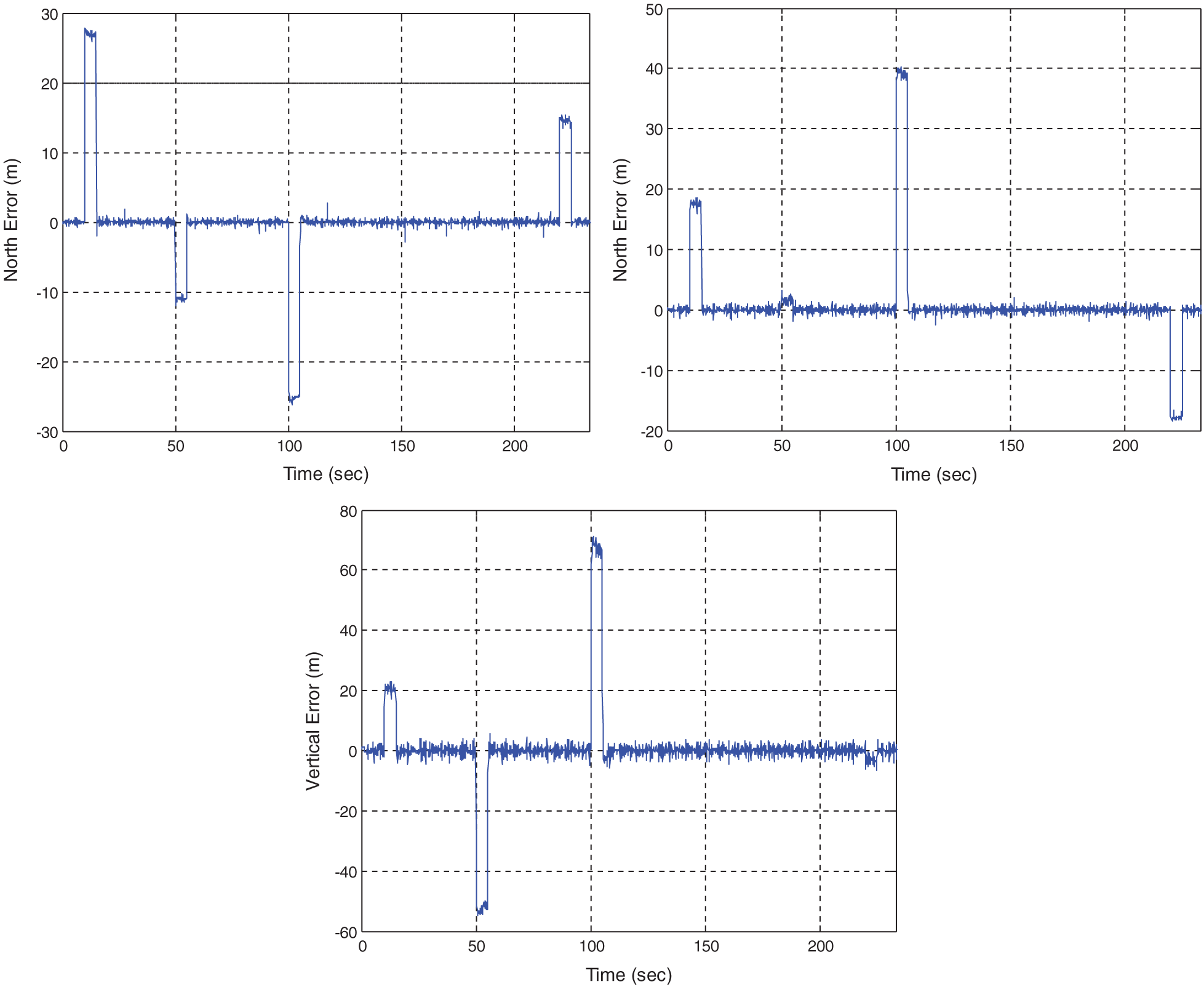
Figure 6: Position errors for Scenario 1 where step type erroneous signals are involved

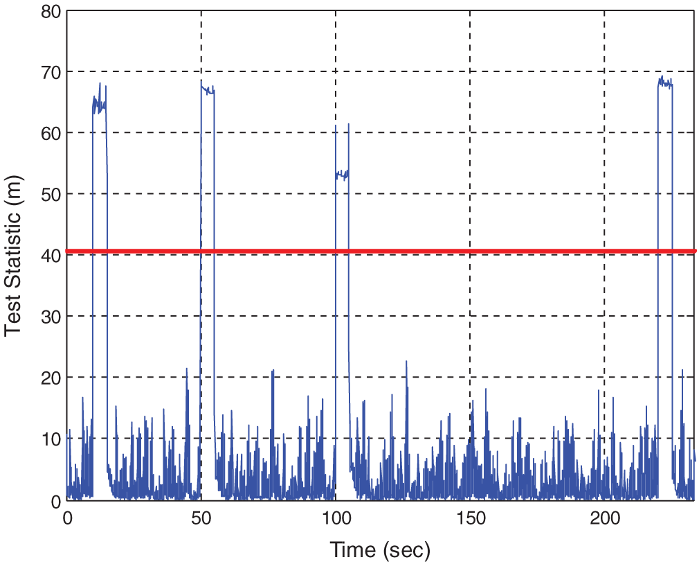
Figure 7: Time history data of test statistic for Scenario 1

(2) Scenario 2: tests for ramp type slowly growing erroneous signals

In the second part of performance test, a slowly growing error is added to Channel 1 in the time interval of 200~233 s. A failure at the rate of 0.3 m/s is used. Fig. 8 provides the error in the east, north and vertical components. Fig. 9 provides the time history data of the test statistic. Fig. 10 shows the time history data of test statistic for the case of slowly growing erroneous signals at the rates of 0.1, 0.2, and 0.3 m/s, respectively. The erroneous signals involved for various rates of failure and the corresponding results are summarized in Tab. 2.

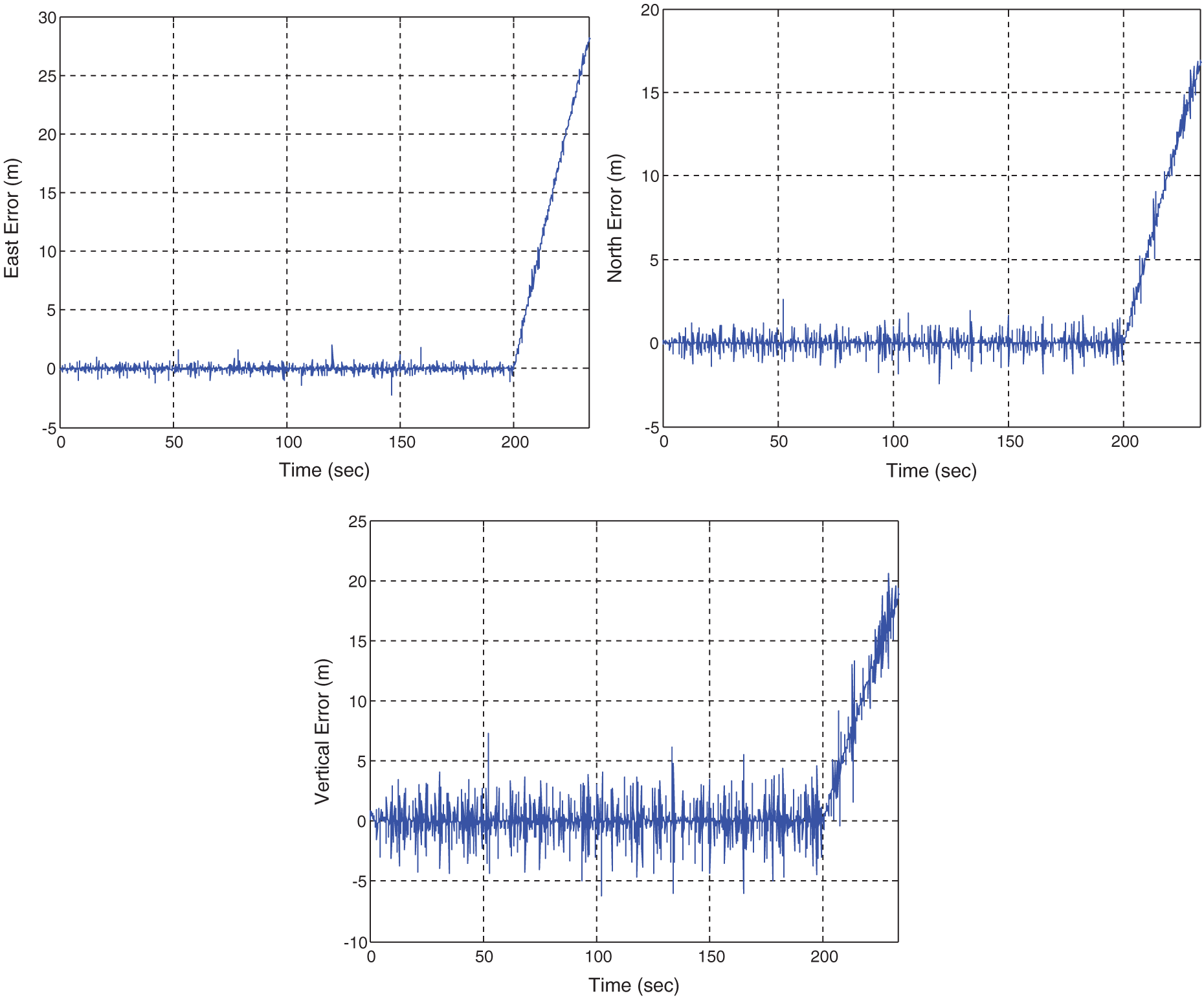
Figure 8: Position errors for the case of 0.3 m/s failure

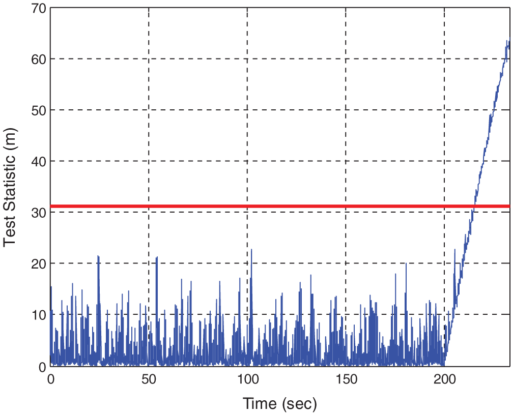
Figure 9: Time history data of the test statistic for the case of 0.3 m/s failure

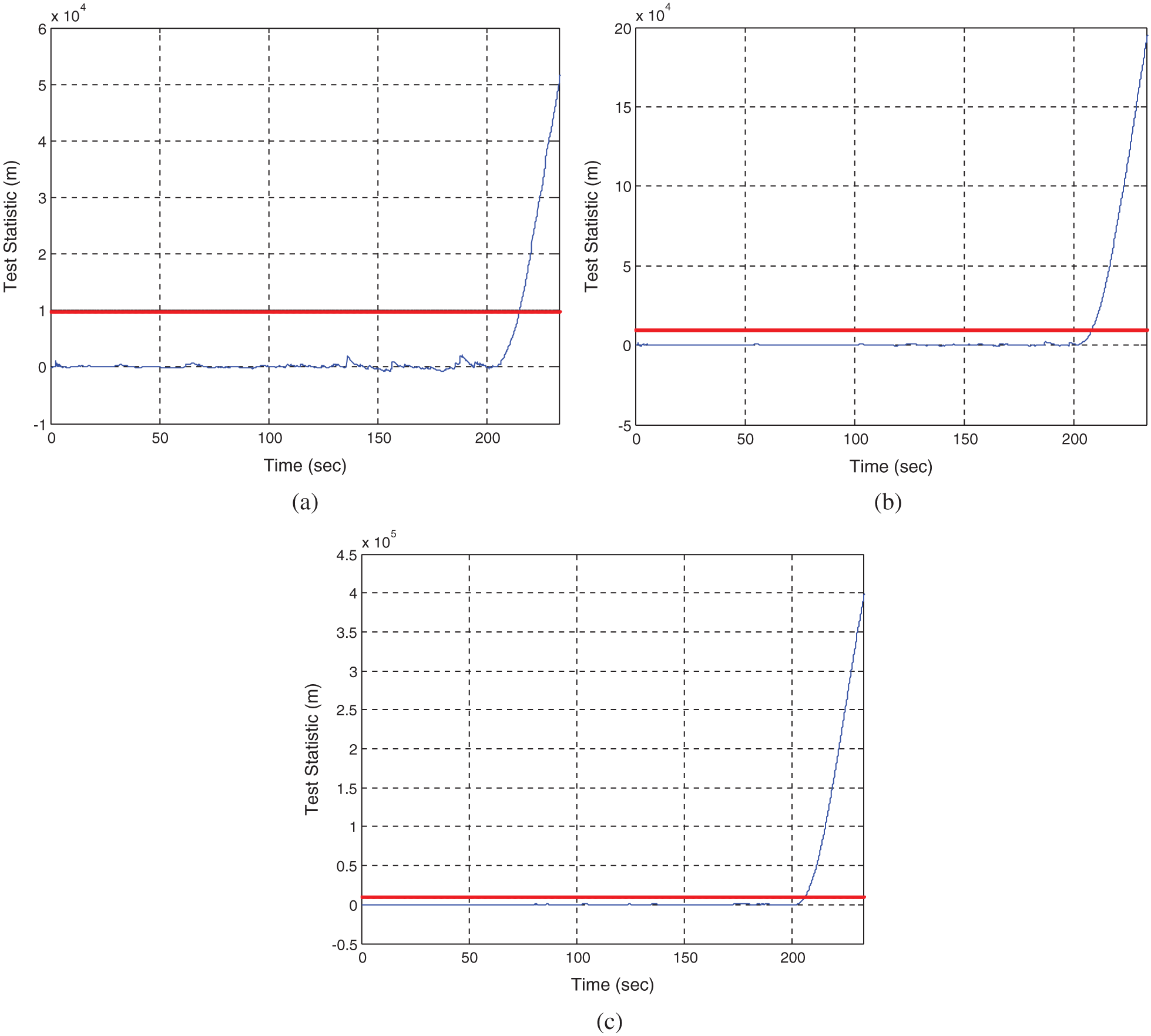
Figure 10: Time history data of the test statistic at three different rates of failure for Scenario 2: (a) 0.1 m/s; (b) 0.2 m/s; (c) 0.3 m/s

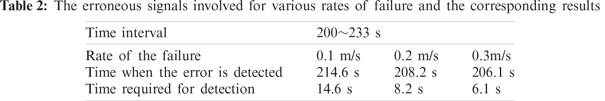
It can be seen that the standard integrity monitoring method does not possess sufficient capability for timely detection of the failure. As for the case of 0.3 m/s failure rate, the conventional integrity monitoring method detects the failure at the time 215.5 s, indicating that the time required for detection is 15.5 s. The rate detector approach can detect the error at the time 206.1 s, meaning that the time required for detection is 6.1 s, which is 9.4 s less than the conventional one. It can be seen that for the case of slowly growing erroneous signals, the detection time required for the proposed method is much more efficient than the conventional approach.

6  Conclusions

For the VTL, the most significant drawback is that failure of tracking in one channel may affect the entire system and possibly lead to loss of lock on all satellites. The integrity monitoring algorithms can be used to detect the possible error in each channel to prevent the spreading of the error into the rest of the channels for the vector tracking loop of the Global Positioning System receivers. Navigation system integrity enables the GPS to provide timely warnings to users when the system should not be used for navigation. Although the standard integrity monitoring algorithm can timely detect the step type erroneous signals, however, it takes much more time in the presence of slowly growing ramp type erroneous signals since the error cannot be detected until the cumulative exceeds the specified threshold.

The integrity monitoring algorithm using a Kalman filter based rate detector is adopted for robustness improvement of the vector tracking loop. The rate detector is realized using a simple Kalman filter and the system failure is detected by detecting the rate of test statistic for determination of whether the ratio exceeds the allowable values. The slowly growing errors can be detected by detecting the rate of the test statistic. The feasibility of the rate detector algorithm has been demonstrated by simulation. Performance assessment and evaluation in integrity monitoring based on the rate detector algorithm as compared to conventional one has been presented. The integrity monitoring based on the rate detector scheme possesses improved efficiency, especially for the slowly growing errors.

Funding Statement: This work has been partially supported by the Ministry of Science and Technology, Taiwan (Grant Numbers MOST 104-2221-E-019-026-MY3 and MOST 109-2221-E-019-010).

Conflicts of Interest: The authors declare that they have no conflicts of interest to report regarding the present study.

This work is licensed under a Creative Commons Attribution 4.0 International License, which permits unrestricted use, distribution, and reproduction in any medium, provided the original work is properly cited.