Computers, Materials & Continua DOI:10.32604/cmc.2021.018955
Article

Computer Geometries for Finding All Real Zeros of Polynomial Equations Simultaneously

Naila Rafiq1, Saima Akram2, Mudassir Shams3,* and Nazir Ahmad Mir1

1Department of Mathematics, NUML, Islamabad, 44000, Pakistan
2Centre for Advanced Studies in Pure & Applied Mathematics, Bahauddin Zakariya University, Multan
3Department of Mathematics and Statistics, Riphah International University I-14, Islamabad, 44000, Pakistan
*Corresponding Author: Mudassir Shams. Email: mudassir4shams@gmail.com
Received: 26 March 2021; Accepted: 27 April 2021

Abstract: In this research article, we construct a family of derivative free simultaneous numerical schemes to approximate all real zero of non-linear polynomial equation. We make a comparative analysis of the newly constructed numerical schemes with a well-known existing simultaneous method for determining all the distinct real zeros of polynomial equations using computer algebra system Mat Lab. Lower bound of convergence of simultaneous schemes is calculated using Mathematica. Global convergence property of the numerical schemes is presented by taking random starting initial approximation and their convergence history are graphically presented. Some real life engineering applications along with some higher degree polynomials are considered as numerical test problems to show performance and efficiency of the derivative free family of numerical methods with comparison of an existing method of same order in literature. Local computational order of convergence, CPU time, graph of computational order of convergence and residual error graphs elaborate efficiency, robustness and authentication of the suggested family of numerical methods in its domain.

Keywords: Polynomials; simultaneous iterative methods; random initial guesses; lower bound; local computational order; CAS-mathematica and mat lab

1  Introduction

One of the most primal problem of science and engineering is locating the zeros of polynomial of degree k with arbitrary real coefficient.

f(x)=∑i=1kaixi,ak≠0.(1)

Let ξ1,…,ξk denote all the simple zeros of Eq. (1). According to Abel’s impossibility theorem [1] “There is no solution in radical to general polynomial with arbitrary co-efficient of degree five or higher” we therefore look toward numerical schemes to approximate zeros of polynomial Eq. (1).

There exist a lot of numerical schemes in literature which approximate single zeros at a time (see, e.g., [2–4]). Here, we consider the following family of numerical schemes [5]:

x(n+1)=y(n)-f(x(n))f′(x(n))((f(x(n)))2f(y(n))+2f(x(n))f(y(n))+β(f(y(n)))3(f(x(n)))3),(2)

where y(n)=x(n)-f(x(n))f′(x(n)) and β∈R.

The numerical scheme Eq. (2) approximate single zero of Eq. (1) at a time.

Beside these single roots finding methods, mathematicians and engineers are interested in simultaneous numerical schemes which approximate all roots simultaneously. More detail on simultaneous methods, their global convergence and parallel implementation on computer algebra system (CAS) and stability are found in [6,7] and reference cite there in [8–14].

Therefore, the main aim of this research article is to construct a derivative free numerical scheme which approximates all real zero of Eq. (1). Using CAS-Mathematica, we find the lower bound of convergence to verify convergence order theoretically. Computational order of convergence [15] and convergence history for random initial approximations are graphed to show the efficiency and performance of numerical schemes as compared to other existing methods of same order. Log of residual graph, graphs of computational order of convergence and local computational order of convergence [16] support the global convergence behavior of our newly constructed numerical scheme for estimating all real zeros of Eq. (1).

2  Construction of Numerical Scheme

Corresponding to numerical schemes

y(n)=x(n)-f(x(n))f′(x(n)),(3)

for approximating all zeros of Eq. (1), the numerical method is

xi(n+1)=xi(n)-f(xi(n))∏j≠ij=1k(xi(n)-xj(n)).(i=1,…,k)(4)

This numerical method is well known Weierstrass method [17] for approximating all zeros of polynomial Eq. (1) having local quadratic convergence. Using in analogical way as above, we convert Eq. (2) into simultaneous method as:

xi(n+1)=yi(n)-f(xi(n))∏j≠ij=1k(xi(n)-xj(n))((f(xi(n)))2f(yi(n))+2f(xi(n))f(yi(n))+β(f(yi(n)))3(f(xi(n)))3),(5)

where yi(n)=xi(n)-f(xi(n))∏j≠ij=1k(xi(n)-xj(n)) and β∈R. Thus, we have constructed here, a new derivative free family of numerical schemes (abbreviated as MD).

Nedzhibov et al. [18] in 2005, present the following cubic convergence derivative free family of simultaneous numerical schemes (abbreviated as ND) as:

xi(n+1)=xi(n)-f(xi(n))∏j≠ij=1k(xi(n)-xj(n))(1+f(yi(n))f(xi(n))-2βf(yi(n))).(6)

2.1 Convergence Analysis

Here, we prove the convergence order of the suggested derivative free family of numerical schemes.

Theorem: Let algebraic polynomial Eq. (1) has k number of simple zeros ξ1,…,ξk and for sufficiently close initial guesses x1(0),…,xk(0) of the zeros, then for arbitrary real parameter β,the numerical scheme MD has third order convergence.

Proof: let ∈i=xi(n)-ξi, ∈i′=yi(n)-ξi, ∈i′′=xi(n+1)-ξi be the errors in xi(n), yi(n) ,xi(n+1) respectively and

Ði=∏j≠ij=1k(xi(n)-ζjxi(n)-xj(n)). (7)

Iterative schemes Eq. (5) can be written as:

xi(n+1)=yi(n)-wi(xi(n))(Ģi+2Ģi2+βĢi3),(8)

where Ģi=f(yi(n))f(xi(n)) and wi(xi(n))=f(xi(n))∏j≠ij=1k(xi(n)-xj(n)).

If we express Eq. (1) as f(xi(n))=(x1(n)-ξ1)…(xk(n)-ξk)=∈i∏j≠ij=1k(xi(n)-ξj), then we have:

f(yi(n))=(y1(n)-ξ1)…(yi(n)-ξi).(9)

Substitution in Eq. (5), we have:

Then, for Ģi, we have:

Ģ i=∈i(1-Ði)∏j≠ij=1k(xi(n)-wi(xi(n))-ξj)∈i∏j≠ij=1k(xi(n)-wi(xi(n))-ξj)=(1-Ði)Ri, (10)

where Ri=xi(n)-wi(xi(n))-ξjxi(n)-wi(xi(n))-ξj. Thus, Eq. (5) become:

∈i′′=∈i′-∈iÐi(Ģ i+2Ģ i2+βĢ i3) (11)

The following relation holds true:

∏j≠ij=1k(xi(n)-ζj)(xi(n)-xj)-1=∑t≠ikεtxi(n)-xt(n)∏j≠it-1(xi(n)-ζt)(xi(n)-xj(n)).(12)

If we assume that, absolute values of all errors are of the same order, say |εi|=|εj|=O(|ε|), then

Ði-1=∑t≠ikεtxi(n)-xt(n)∏j≠it-1(xi(n)-ζt)(xi(n)-xj(n))=O(|ε|) (13)

holds. Using ÐiRi=∏j≠ij=1k(xi(n)-wi(xi(n))ξjxi(n)-xj(n)), we have:

Thus,

∈i′′=∈i∑t≠ik∈txi(n)-xt∏j≠it-1(xi(n)-ζt)(xi(n)-xj(n))(O(|∈|)+2O(|∈|2)Ri+O(|∈|2)Ri3β)=O(∈3).(14)

Hence, the theorem is proved.

2.2 Using CAS-Mathematica for Finding Lower Bound of Convergence

Consider

f(x)=(x-φ1)(x-φ2)(x-φ3)(15)

and the first component H(x(n)) of iterative scheme Eq. (5) to find zeros of Eq. (15), simultaneously. In order to find lower bound of convergence, we have to express the differential of an operator H(x(n)) in terms of their partial derivate of its component as Hi(x):

and to so on.

The lower bound of the convergence is obtained until the first non-zero element of row is found zero (see [19]). The Mathematica program is given for each of the considered method as:

•   MD method

In[1]:=D[H1[x1, x2, x3], x1]/.{x1→φ1,x2→φ2,x3→φ3}

Out[1]:=0

In[2]:=D[H1[x1, x2, x3], x2]/.{x1→φ1,x2→φ2,x3→φ3}]

Out[2]:=0

In[2]:=D[H1[x1, x2, x3], x2]/.{x1→φ1,x2→φ2,x3→φ3}]

Out[2]:=0

In[34]:=Simplify[D[H1[x1, x2, x3], x1,x1,x1,x2]/.{x1→φ1,x2→φ2,x3→φ3}]

Out[34]:=6(-1+φ3)φ12φ33.

•   ND method

where y=x-f(x)∏j=1j≠in(xi-xj) and β∈R.

In[1]:=D[H1[x1, x2, x3], x1]/.{x1→φ1,x2→φ2,x3→φ3}]

Out[1]:=0

⋮

In[39]:=Simplify[D[H1[r1, r2, r3], r1,r3,r1,r2]/.{x1→φ1,x2→φ2,x3→φ3}]

Out[39]:=-6(2-2φ3)φ1φ32

3  Numerical Results

Here, some numerical examples from [20,21] are considered with and without random initial approximation to estimate all real zeros of polynomial equation of higher degree. All the computations are performed using Mat Lab R@2011 with 64 digits floating point arithmetic. We take ∈=10-30 as tolerance and use the following stopping criteria

where ei represents the absolute error. We compare our iterative schemes MD with ND of the same convergence order. In all numerical calculations, we take β=2.

Example 1: Consider a stirred tank reactor (SCRT) in which two items A and R are feed in reactor at Q and q-Q rate respectively. A complex reaction

a+r→b;b+r→c;c+r→r;c+r→e, develops the following function

hc2.98(x+2.25)(x+1.45)(x+2.85)2(x+4.35)=1.(16)

We obtained an algebraic polynomial equation of degree 4 by taking ℏc=0 in Eq. (16)

with exact roots:

Convergence history and computational order of convergence graph (Figs. 1, 4, 7 and 10) of numerical schemes ND, MD are obtained by taking the following random initial guessed valued in our computer program i.e.,

where X1=[xi(0),i=1,…,4]. Using random initial guessed value X1, the iterative scheme MD converges to exact zeros after 100 iteration by consuming 16.848368 s CPU time while ND converges after 155 iterations and consumes 37.249147 s.

Figure 1: Shows convergence history of numerical scheme MD for polynomial equation f1(x)

Figure 2: Shows convergence history of numerical scheme MD for polynomial equation f2(x)

Figure 3: Shows convergence history of numerical scheme MD for polynomial equation f3(x)

Figure 4: Shows convergence history of numerical scheme ND for polynomial equation f1(x)

Figure 5: Shows convergence history of numerical scheme ND for polynomial equation f2(x)

Figure 6: Shows convergence history of numerical scheme ND for polynomial equation f3(x)

Figure 7: Shows computational order of convergence of numerical scheme MD for polynomial equation f1(x)

Figure 8: Shows computational order of convergence of numerical scheme MD for polynomial equation f2(x)

Figure 9: Shows computational order of convergence of numerical scheme MD for polynomial equation f3(x)

Figure 10: Shows computational order of convergence of numerical scheme ND for polynomial equation f1(x)

Convergence rates increase by taking the following initial guessed value:

The numerical results are presented in Tabs. 1–6. In all Tabs. 1–6, CO presents convergence order, CPU, presents CPU time and local computational order of convergence (LCOC) by σ.

Example 2: Consider

f2(x)=x5-3x4-23x3+51x2+94x-120(17)

with exact roots:

For convergence history and computational order of convergence graph (Figs. 2, 5, 8 and 11) of numerical schemes ND, MD, we used the following initial guessed valued in our computer program i.e.,

where X2=[xi(0),i=1,…,5]. Using random initial guessed values X2, the iterative scheme MD converges to exact zeros after 92 iteration by consuming 27.056098 s CPU time while ND converges after 98 iterations and consumes 31.444833 s.

Convergence rates increase by taking the following initial guessed value:

Example 3: Consider

f3(x)=x7-27x6+282x5-1410x4+3249x3-1923x2-3532x+3360(18)

with exact roots:

For convergence history and computational order of convergence graph (Figs. 3, 6, 9 and 12) of numerical schemes ND, MD are obtained by taking the following initial guessed valued in our computer program i.e.,

where X3=[xi(0),i=1,…,7]. Using random initial guessed value X3, the iterative scheme MD converges to exact zero after 19 iterations by consuming 13.7714 s CPU time while ND converges after 23 iterations and consumes 18.120062 s.

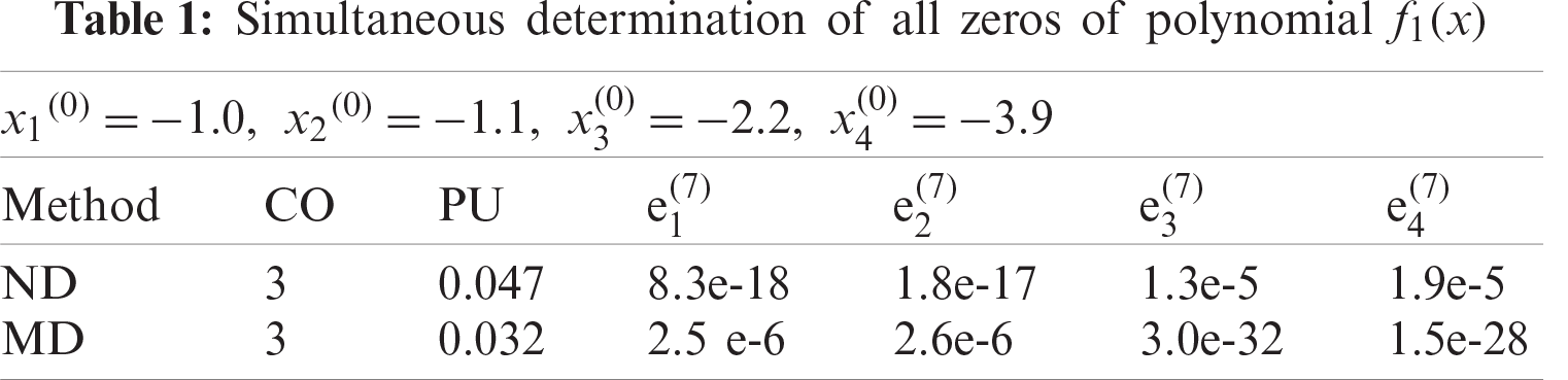
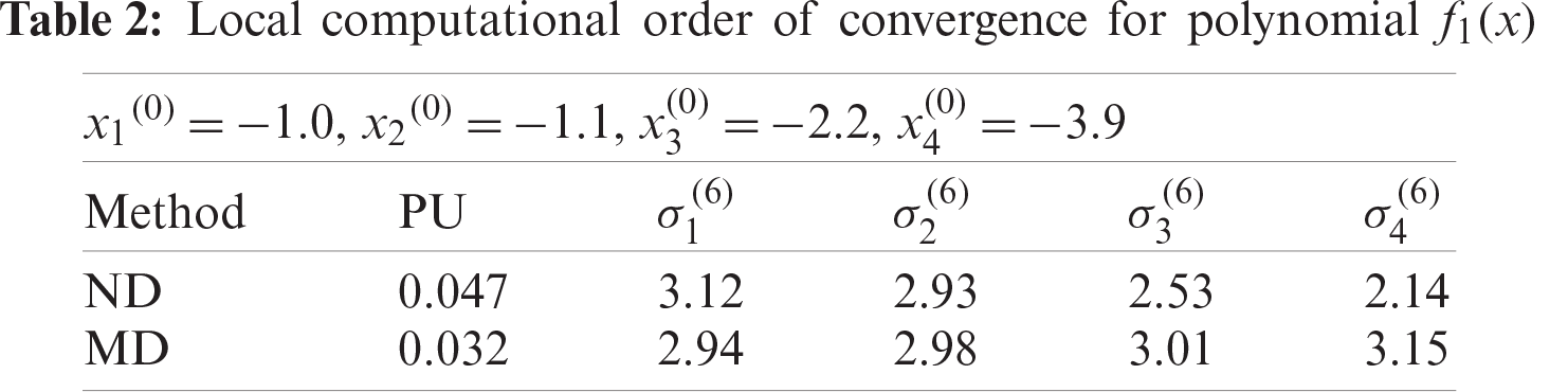
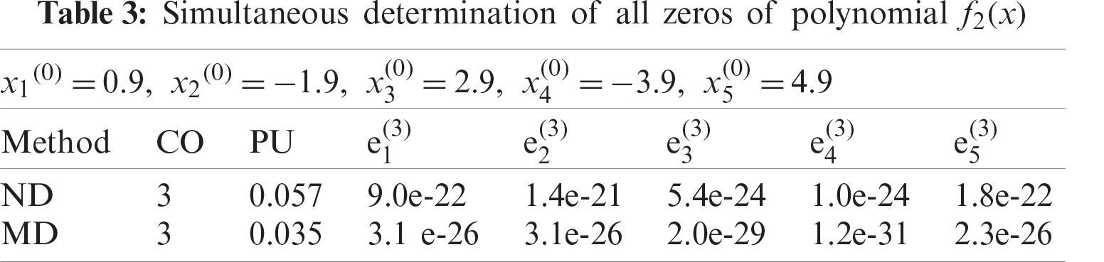
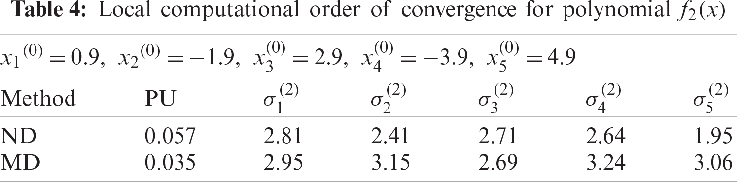
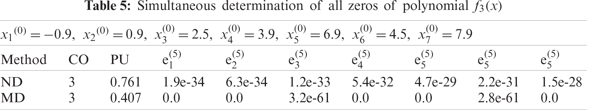
Figure 11: Shows computational order of convergence of numerical scheme ND for polynomial equation f2(x)

Figure 12: Shows computational order of convergence of numerical scheme ND for polynomial equation f3(x)

Figure 13: Shows residual fall for iterative method MD and ND for polynomial f1(x) respectively

Figure 14: Shows residual fall for iterative method MD and ND for polynomial f2(x) respectively

Figure 15: Shows residual fall for iterative method MD and ND for polynomial f3(x) respectively

Convergence rates increase by taking the following initial guessed value:

4  Conclusions

Here, we have developed a family of derivative free method for approximating all real zeros of polynomial. Lower bound of convergence of iterative methods MD and ND are calculated using CAS-Mathematica. Using Mat Lab, we graph convergence history and computational order of convergence. From Tabs. 1–6 and Figs. 1–15, we observe that our method MD is much better in terms of convergence history, computational order of convergence, numerical results, log of residual and local computational order of convergence as compared to ND method.

Funding Statement: The authors received no specific funding for this study.

Conflicts of Interest: The authors declare that they have no conflicts of interest to report regarding the present study.

This work is licensed under a Creative Commons Attribution 4.0 International License, which permits unrestricted use, distribution, and reproduction in any medium, provided the original work is properly cited.