DOI:10.32604/cmc.2021.015504
| Computers, Materials & Continua DOI:10.32604/cmc.2021.015504 | |
| Article |
An Optimized Approach to Vehicle-Type Classification Using a Convolutional Neural Network
1Department of Information Technology, College of Computer, Qassim University, Buraidah, 51452, Saudi Arabia
2Department of Computer Science, Islamia College University, Peshawar, Pakistan
*Corresponding Author: Noreen Fayyaz Khan. Email: noreen.fayyaz@fu.edu.pk
Received: 25 November 2020; Accepted: 02 March 2021
Abstract: Vehicle type classification is considered a central part of an intelligent traffic system. In recent years, deep learning had a vital role in object detection in many computer vision tasks. To learn high-level deep features and semantics, deep learning offers powerful tools to address problems in traditional architectures of handcrafted feature-extraction techniques. Unlike other algorithms using handcrated visual features, convolutional neural network is able to automatically learn good features of vehicle type classification. This study develops an optimized automatic surveillance and auditing system to detect and classify vehicles of different categories. Transfer learning is used to quickly learn the features by recording a small number of training images from vehicle frontal view images. The proposed system employs extensive data-augmentation techniques for effective training while avoiding the problem of data shortage. In order to capture rich and discriminative information of vehicles, the convolutional neural network is fine-tuned for the classification of vehicle types using the augmented data. The network extracts the feature maps from the entire dataset and generates a label for each object (vehicle) in an image, which can help in vehicle-type detection and classification. Experimental results on a public dataset and our own dataset demonstrated that the proposed method is quite effective in detection and classification of different types of vehicles. The experimental results show that the proposed model achieves 96.04% accuracy on vehicle type classification.
Keywords: Vehicle classification; convolutional neural network; deep learning; surveillance
Surveillance systems have achieved good results in terms of security. Image analysis, such as detecting a moving vehicle in an image, is a challenging task that can be solved by analyzing the foreground [1]. Dramatic improvements have been observed in the areas of speech recognition and document recognition genomics for automation technologies [2]. Major issues in surveillance systems include brightness, lighting, occlusion of shadows, and fragmentation, and all have a negative impact on objects to be detected [3,4]. Much research has been done on vehicle-type recognition systems that include handcrafted feature-extraction techniques such as speeded-up robust features (Surf), local binary patterns (LBPs), histogram of gradients (HOG) [5], annular coil, radar detection radio wave or infrared contour scanning, vehicle weight, and laser sensor measurement [6,7]. Automatic detection and classification of vehicle types using a convolutional neural network (CNN) is an unsolved problem. Deep CNNs [8,9], as well as extensively annotated datasets (e.g., ImageNet [10]), have brought remarkable progress in image recognition. Deep learning approaches are useful for feature extraction, and selection without prior knowledge has been investigated [11]. The most popular form of deep learning model, the CNN, consists of a series of convolutional layers followed by pooling layers and fully connected layers. The convolutional layer forms feature maps within which each unit is associated with a set of weights called filters. The pooling layer computes the sampling feature maps by summarizing the presence of feature maps. The fully connected layers are used for classification. All the weights are updated by gradient-based learning.
In this research, we employed the AlexNet CNN architecture and customized its network layers and options according to our classification objectives. Image features are the primary elements for any object detection. The model extracts the features from the training dataset through convolutional and pooling layers. The proposed model works on backpropagation gradients that help to reduce the discrepancy between the correct output and that produced by the system. The CNN helps learns the semantics of the categories of vehicle images so as to produce accurate detection and classification results.
The key contributions of this work follow.
• Vehicles are automatically detected and classified irrespective of brightness, lighting, occlusion of shadows, and fragmentation.
• The AlexNet model is used to classify vehicle types by customizing layers according to the problem domain.
• Deep learning helps to automatically learn features through filters in the convolutional layer.
• The system helps in vehicle-tracking systems in commercial parking areas and assists in counting the number of vehicles on a road.
The classification of vehicles is a challenging problem in the field of vision-based surveillance. There is huge within-class variability in vision-based vehicle detection systems, as vehicles may differ in color, size, and shape, illumination can vary, and background can be cluttered. Furthermore, the appearance of vehicles depends on their posture and might be affected by neighboring objects [12]. Shallow classification models are used by traditional image classification systems, such as support vector machine (SVM) [13], Bayesian [14], random forest (RF) [15], and boosting [16], to extract features for classification, such as local binary patterns (LBP), histogram of oriented gradients (HOG) [17], and scale-invariant feature transform (SIFT) [18]. These methods rely on hand-designed features. Shallow models are trained by original training data with limited fitness in representation learning [8]. Fu et al. [19] proposed a hierarchical multi-SVM method for vehicle classification. Other methods include a real-time system for multiple vehicle detection and classification using a Gaussian mixture model with hole filling algorithm (GMMHF), Gabor kernel for feature extraction, and multi-class vehicle classification [20]. Use of a CNN to classify images marks a massive revolution. Some deep learning techniques surpass humans on tasks like face recognition and image classification [21–23]. Machine learning techniques have seen successful application, and are considered the best choice compared to neural networks and support vector machine for vehicle detection and classification [24]. Roadside LiDAR sensors [25], frequency-modulated continuous-wave (FMCW) radar signals [26], sensors for vehicle classification and counting [27], and distributed optical sensing technology in vibration-based vehicle classification systems [28] also play a significant role in vehicle classification.
Increased traffic has become an issue in many towns and cities, causing serious traffic congestion problems. This paper develops a simple and efficient vehicle-type recognition system using a CNN model. The framework, as shown in Fig. 1, includes three steps: a) preparing the dataset; b) feature extraction by CNN; and c) classification of test data.

Figure 1: Proposed framework for vehicle-type detection and classification
For effective learning patterns, a huge amount of data is required for a deep learning-based approach. The effective deployment of deep learning models requires abundant high-quality data [13]. To attain the desired accuracy, we apply four data-augmentation techniques to extend the dataset. Tab. 1 shows the extended dataset. Data augmentation includes flipping, skewness, rotation, and translations for geometric transformation invariance. The second column in Tab. 1 lists techniques, and the third column shows their invariance parameters.
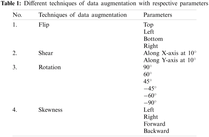
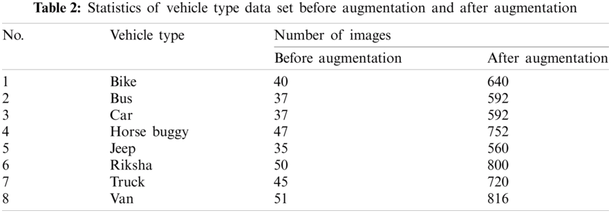
The four augmentation techniques and 16 parameters extend each sample to form 16 samples. Tab. 2 shows eight classes of vehicles: bike, bus, car, horse buggy, jeep, rickshaw, truck, and van. The third column presents the number of images of each vehicle type before and after augmentation. The purpose of augmentation is the effective deployment of the deep learning model. It also helps to avoid overfitting and memorizes the targeted details of the training images. All of the images in the dataset are preprocessed to the size of 227 (width)
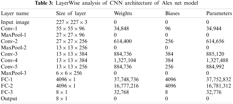
In the proposed system, the AlexNet CNN architecture is fine-tuned [9], as shown in Fig. 2. AlexNet has eight layers. Five are convolutional (conv) layers, where conv1, conv2, conv3, and conv4 are followed by the max-pooling layer, and the last three are fully connected layers. Dataset features are extracted by applying a deep CNN model containing manifold convolutional layers. A feature map (fmap) that represents a higher-level abstraction of the input data is generated by each convolutional layer. The fmaps of the starting convolutional layers extract low-level features such as color, shape, corners, and edges, and the fmap of the last convolutional layer includes the high-level features, which are forwarded to the fully connected layers for classification. Tab. 3 provides an architectural analysis of each layer of the fine-tuned AlexNet model. The first convolutional layer is produced by applying a filter of size

Figure 2: Architecture of fine-tuned Alex net CNN mode
The number of parameters of the convolutional layer is formulated as
where
The size (O) of the output tensor (image) of the maximum pool layer is formulated as
where
Ps = pool size.
where
Fig. 3 shows the features extracted from an image by the deep CNN model. In the first convolutional layer, conv1 extracts the edges and blobs, conv2 and conv3 extract the texture, conv4 and conv5 extract the object parts, and the last fully connected layer detects the object classes.

Figure 3: Features extraction of the 5 convolutional layers

Figure 4: Random images of vehicles from training dataset
3.3 Vehicle Type Classification
We discuss the classification of multiple categories of vehicles through several experiments on the dataset. The parameters used in the AlexNet model were customized for optimal results. The network was trained by splitting the dataset into 70% for training and 30% for validation. The activations of the pre-trained model learned patterns in different datasets through transfer learning. All the layers of the pre-trained network were extracted, except the last three layers, which were configured for 1000 classes. We fine-tuned these three layers for our classification problem. Training was optimized by setting the minibatch size to 7, maximum epochs to 35, and learning rate to 1e −5. Experiments were evaluated using MATLAB with a deep learning toolbox. The proposed model was trained on a GPU. The elapsed time was 47 s. The model took random images from the validation dataset and accurately labeled them according to their type. Fig. 4 shows random images from the training dataset, classified with their class labels from the testing (validation) dataset. Images were correctly classified according to their type, except the one in the third row and first column; this means that the model needed more data for training of that particular image to give better results.
We present accuracy as the evaluation method. This is computed with the help of a confusion matrix, as shown in Fig. 5, which shows the performance of the algorithm for each class of vehicle. Accuracy shows the percentage of the correctly predicted class in the entire testing dataset, and is formulated as

Figure 5: Confusion matrix of the optimized vehicle classification approach
We discuss the experimental assessment for the detection and classification of vehicle types. We evaluated the dataset with the stochastic gradient descent with momentum (SGDM) and adaptive moment estimation (Adam) algorithms with epochs ranging from 10 to 40. The optimizers were used to change the weights of CNN to reduce the losses. During training, optimization is a key component that helps the model to adjust weights during backpropagation [29,30], which is formulated as:
where j = 0, 1 represents the feature index number.
4.1 Results with SGDM Optimizer
The gradient vectors were accelerated in the right direction, leading to fast convergence with the help of SGD with momentum (SGDM) [31]. We trained the model with an SGDM optimizer by applying different epochs. The SGDM algorithm is formulated as:
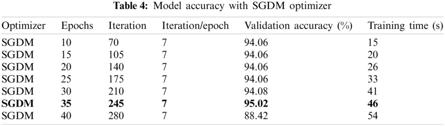
The model first trained with 10 epochs, giving 94.06% accuracy with a collapse time of 15 s. For better performance, the model was trained further with 15, 20, 25, 30, 35, and 40 epochs. The number of iterations is directly proportional to the number of epochs. It is observed that the system showed the best result on epoch 35, with 95.02% accuracy. System performance then started to decline due to overfitting.
4.2 Results with ADAM Optimizer
The Adam optimizer iteratively updated the network weights in the training dataset [29]. After training the model with an SGDM optimizer, it was assessed with an Adam optimizer for improved accuracy. The Adam algorithm is formulated as:
The model was trained with the same number of epochs as previously described. It is observed that the best result obtained with the Adam optimizer was at 35 epochs, with 90.10% accuracy. The literature shows that SGDM performs better than Adam in reducing the loss [31]. The experimental results in Tabs. 4 and 5 show that the accuracy of the model with SGDM was 95.02% with 46 s training time, while the accuracy with Adam was 90.10%, with a training time of 50 s. Therefore, SGDM provided better accuracy than Adam.

4.3 Model Accuracy with SGDM Optimizer and Different Learning Rates
For more convincing results, the model was evaluated with different learning rates with 35 epochs, which gives the best results in Tabs. 4 and 5. The learning rate determines the step size at each iteration in an optimization algorithm. It is a tuning parameter that minimizes the loss function [32,33]. The model was trained again with SGDM and 35 epochs, with learning rates ranging from 1e −3 to 1e −6. The learning rate affected the quick convergence of the model toward local minima. It improved the performance of our model from 95.02% to 96.04% by adjusting the learning rate

Figs. 6 and 7 show the training progress of the model used in this study. The upper graphs show the accuracy of the model, which is measured by the performance estimated on a set of samples from the test data. The lower graph shows the loss of the model. It is computed by the gradient of the loss function concerning the parameters [34], and it shows the gap between the actual and expected output scores. During the first epoch, the rate of accuracy increased from 20% to 80% due to backpropagating gradients that updated the maximum weights of the filters in our classification task. For this, SGDM was set at a learning rate of 0.00001. This allowed for fine-tuning to make progress in the remaining epochs. The accuracy fluctuated between 80% and 95% because the maximum number of weights had been trained. Similarly, during the first epoch, the loss decreased dramatically from 2.5 to 0.5 in each iteration; the model minimized the error by updating the weights. By the completion of 35 epochs, the proposed model had 96.04% accuracy on the validation dataset.

Figure 6: Best result with SGDM optimizer

Figure 7: Best result with Adam optimizer
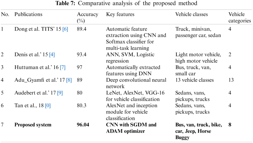
We evaluated the proposed method against state-of-the-art deep learning methods [35]. Dong used CNN for automatic feature extraction by classifying four categories of vehicles, with 89.4% accuracy. Another method, based on a comparative analysis of ANN, SVM, and logistic regression, classified small vehicles and big vehicles with 93.4% accuracy. Huttuman automatically extracted features using deep neural networks, and classified four classes of vehicles with 97% accuracy. Adu Gyamfi used a deep CNN to classify 13 vehicle classes with 89% accuracy. The last two methods, as mentioned in Tab. 7, used LeNet, AlexNet, VGG-16, and an inception module for vehicle classification, with respective accuracies of 80% and 80.3% which are much lower than those of our proposed system. Our method achieved better accuracy than all of the above methods except the Huttuman approach, whose accuracy was high, but could classify only four classes of vehicles while the proposed method classified eight classes of vehicles. Tab. 7 shows a comparative analysis of the proposed method.
Our method detects and classifies multiple classes of vehicles through a deep learning model. It can help in vehicle tracking systems for surveillance in big parking slots where security is a concern. It can help solve traffic issues by directing large vehicles to one side of a road and keep the traffic moving by knowing what vehicles are ahead in a queue. This research will help by classifying the vehicles in parking zones and automatically allocate tickets according to vehicle types. The accuracy of the model can be improved by increasing the sample size.
Acknowledgement: We acknowledge the overall paper editing support by Dr. Sheroz Khan and Dr. Muhammad Islam, Department of Electrical Engineering and Renewable Engineering, College of Engineering & Information Technology, Onaizah Colleges, Al-Qassim, Saudi Arabia;2053, Saudi Arabia. We thank LetPub (www.letpub.com) for its linguistic assistance during the preparation of this manuscript.
Funding Statement: This work is supported by the Information Technology Department, College of Computer, Qassim University, 6633, Buraidah 51452, Saudi Arabia.
Conflicts of Interest: The authors declare that they have no conflicts of interest to report regarding the present study.
1. Y. L. Tian, M. Lu and A. Hampapur, “Robust and efficient foreground analysis for real-time video surveillance,” in IEEE Computer Society Conf. on Computer Vision and Pattern Recognition, vol. 1, pp. 1182–1187, 2005. [Google Scholar]
2. Y. Sun, Y. Liu, G. Wang and H. Zhang, “Deep learning for plant identification in natural environment,” Computational Intelligence and Neuroscience, vol. 2017, no. 4, pp. 1–6, 2017. [Google Scholar]
3. P. Maja, A. Pentland, A. Vinciarelli, R. Cucchiara, M. Daoudi et al., “Joint ACM workshop on human gesture and behavior understanding,” in Proc. of the 19th ACM Int. Conf. on Multimedia, vol. 19, pp. 615–616, 2011. [Google Scholar]
4. Y. L. Tian, R. S. Feris, H. Liu, A. Hampapur and M. T. Sun, “Robust detection of abandoned and removed objects in complex surveillance videos,” IEEE Transactions on Systems, Man, and Cybernetics, Part C (Applications and Reviews) 41, vol. 5, pp. 565–576, 2010. [Google Scholar]
5. J. Deng, W. Dong, R. Socher, L. J. Li, K. Li et al., “Imagenet: A large-scale hierarchical image database,” in IEEE Conf. on Computer Vision and Pattern Recognition, Florida, USA, pp. 248–255, 2009. [Google Scholar]
6. W. Zhan and Q. Wan, “Real-time and automatic vehicle type recognition system design and its application,” in Int. Symp. on Intelligence Computation and Applications, Wuhan, China, pp. 200–208, 2012. [Google Scholar]
7. S. Xiong, Research of Automobile Classifying Method Based on Inductive Loop. Hunan, China: ChangSha University of Science and Technology, pp. 2–5, 2009. [Google Scholar]
8. A. Krizhevsky, I. Sutskever and G. E. Hinton, “Imagenet classification with deep convolutional neural networks,” Communications of the ACM 60, vol. 6, no. 6, pp. 84–90, 2017. [Google Scholar]
9. V. Sze, Y. H. Chen, T. J. Yang and J. S. Emer, “Efficient processing of deep neural networks: A tutorial and survey,” Proc. of the IEEE, vol. 12, pp. 2295–2329, 2017. [Google Scholar]
10. O. Russakovsky, J. Deng, H. Su, J. Krause, S. Satheesh et al., “Imagenet large scale visual recognition challenge,” International Journal of Computer Vision 115, vol. 3, no. 3, pp. 211–252, 2015. [Google Scholar]
11. H. C. Shin, H. R. Roth, M. Gao, L. Lu, Z. Xu et al., “Deep convolutional neural networks for computer-aided detection: CNN architectures, dataset characteristics and transfer learning,” IEEE Transactions on Medical Imaging 35, vol. 5, no. 5, pp. 1285–1298, 2016. [Google Scholar]
12. X. Wen, L. Shao, Y. Xue and W. Fang, “A rapid learning algorithm for vehicle classification,” Information Sciences, vol. 295, no. 3, pp. 395–406, 2015. [Google Scholar]
13. D. Zhao, Y. Chen and L. Lv, “Deep reinforcement learning with visual attention for vehicle classification,” IEEE Transactions on Cognitive and Developmental Systems 9, vol. 4, pp. 356–367, 2016. [Google Scholar]
14. D. P. Pietro and F. Hristea, “Unsupervised word sense disambiguation with N-gram features,” Artificial Intelligence Review 41, vol. 2, no. 2, pp. 241–260, 2014. [Google Scholar]
15. A. Liaw and M. Wiener, “Classification and regression by random forest,” R News, vol. 2, no. 3, pp. 18–22, 2002. [Google Scholar]
16. J. Shotton, J. Winn, C. Rother and A. Criminisi, “Textonboost for image understanding: Multi-class object recognition and segmentation by jointly modeling texture, layout, and context,” International Journal of Computer Vision, vol. 81, no. 1, pp. 2–23, 2009. [Google Scholar]
17. N. Dalal and B. Triggs, “Histograms of oriented gradients for human detection,” in 2005 IEEE Computer Society Conf. on Computer Vision and Pattern Recognition, San Diego, CA, USA, IEEE, 2005. [Google Scholar]
18. D. G. Lowe, “Distinctive image features from scale-invariant keypoints,” International Journal of Computer Vision, vol. 60, no. 2, pp. 91–110, 2004. [Google Scholar]
19. H. Fu, H. Ma, Y. Liu and D. Lu, “A vehicle classification system based on hierarchical multi-SVMs in crowded traffic scenes,” Neuro Computing, vol. 211, pp. 182–190, 2016. [Google Scholar]
20. A. Nurhadiyatna, A. L. Latifah and D. Fryantoni, “Gabor filtering for feature extraction in real time vehicle classification system,” in 9th Int. Symp. on Image and Signal Processing and Analysis, Zagreb, Croatia, IEEE, 2015. [Google Scholar]
21. H. Kaiming, X. Zhang, S. Ren and J. Sun, “Deep residual learning for image recognition,” in Proc. of the IEEE Conf. on Computer Vision and Pattern Recognition, Las Vegas, NV, USA, pp. 770–778, 2016. [Google Scholar]
22. S. Pierre, D. Eigen, X. Zhang, M. Mathieu, R. Fergus et al., “Overfeat: Integrated recognition, localization and detection using convolutional networks,” ArXiv, vol. 13, no. 12, pp. 62–92, 2013. [Google Scholar]
23. Y. Sun, X. Wang and X. Tang, “Deep learning face representation from predicting 10,000 classes,” in Proc. of the IEEE Conf. on Computer Vision and Pattern Recognition, Columbus, OH, USA, 2014. [Google Scholar]
24. K. Denis, R. Hostettler, W. Birk and Evgeny Osipov, “Comparison of machine learning techniques for vehicle classification using road side sensors,” in IEEE 18th Int. Conf. on Intelligent Transportation Systems, Rio de Janeiro, Brazil, 2015. [Google Scholar]
25. J. Wu, H. Xu, Y. Zheng, Y. Zhang, B. Lv et al., “Automatic vehicle classification using roadside LiDAR data,” Transportation Research Record, vol. 2673, no. 6, pp. 153–164, 2019. [Google Scholar]
26. C. Samuele, L. Facheris, F. Cuccoli and S. Marinai, “Vehicle classification based on convolutional networks applied to FMCW radar signals,” in Italian Conf. for the Traffic Police, Berlin, Germany, Springer, 2017. [Google Scholar]
27. W. Balid, H. Tafish and H. H. Refai, “Intelligent vehicle counting and classification sensor for real-time traffic surveillance,” IEEE Transactions on Intelligent Transportation Systems, vol. 19, no. 6, pp. 1784–1794, 2017. [Google Scholar]
28. H. Zhao, D. Wu, M. Zeng and S. Zhong, “A vibration-based vehicle classification system using distributed optical sensing technology,” Transportation Research Record, vol. 2672, no. 43, pp. 12–23, 2018. [Google Scholar]
29. E. M. Dogo, O. J. Afolabi, N. I. Nwulu and B. Twala, “A comparative analysis of gradient descent-based optimization algorithms on convolutional neural networks,” in 2018 Int. Conf. on Computational Techniques, Electronics and Mechanical Systems, New York, US, IEEE, 2018. [Google Scholar]
30. L. Bottou, “Stochastic gradient descent tricks,” in Neural Networks: Tricks of the Trade, Berlin, Germany: Springer, pp. 421–436, 2012. [Google Scholar]
31. L. Bottou, “Large-scale machine learning with stochastic gradient descent,” in Proc. of COMPSTAT’2010, France, pp. 177–186, 2010. [Google Scholar]
32. S. Benard and S. Y. Arnob, “Discriminator-actor-critic: Addressing sample inefficiency and reward bias in adversarial im-itation learning,” ICLR Reproducibility-Challenge, 2019. [Google Scholar]
33. G. Ozbulak, Y. Aytar and H. K. Ekenel, “How transferable are CNN-based features for age and gender classification,” in Int. Conf. of the Biometrics Special Interest Group, Darmstadt, Germany, IEEE, 2016. [Google Scholar]
34. L. Yann, L. Bottou, Y. Bengio and P. Haffner, “Gradient-based learning applied to document recognition,” Proc. of the IEEE, vol. 86, no. 11, pp. 2278–2324, 1998. [Google Scholar]
35. M. Won, “Intelligent traffic monitoring systems for vehicle classification: A survey,” IEEE Access, vol. 8, pp. 73340–73358, 2020. [Google Scholar]
36. Z. Dong, Y. Wu, M. Pei and Y. Jia, “Vehicle type classification using a semi-supervised convolutional neural network,” IEEE Transactions on Intelligent Transportation Systems, vol. 16, no. 4, pp. 2247–2256, 2015. [Google Scholar]
37. H. Huttunen, F. S. Yancheshmeh and K. Chen, “Car type recognition with deep neural networks,” in IEEE Intelligent Vehicles Symp., Gothenburg, Sweden, IEEE, 2016. [Google Scholar]
38. A. Gyamfi, Y. Okyere, S. K. Asare, A. Sharma and T. Titus, “Automated vehicle recognition with deep convolutional neural networks,” Transportation Research Record, vol. 2645, no. 1, pp. 113–122, 2017. [Google Scholar]
39. N. Audebert, B. Le Saux and S. Lefèvre, “Segment-before-detect: Vehicle detection and classification through semantic segmentation of aerial images,” Remote Sensing, vol. 9, no. 4, pp. 368, 2017. [Google Scholar]
40. Y. Tan, Y. Xu, S. Das and A. Chaudhry, “Vehicle detection and classification in aerial imagery,” in 25th IEEE Int. Conf. on Image Processing, Athens, Greece, IEEE, 2018. [Google Scholar]
 | This work is licensed under a Creative Commons Attribution 4.0 International License, which permits unrestricted use, distribution, and reproduction in any medium, provided the original work is properly cited. |