DOI:10.32604/cmc.2021.017266
| Computers, Materials & Continua DOI:10.32604/cmc.2021.017266 | |
| Article |
Bayesian Rule Modeling for Interpretable Mortality Classification of COVID-19 Patients
Software Department, Gachon University, Seongnam, 13120, Korea
*Corresponding Author: Myung-Mook Han. Email: mmhan@gachon.ac.kr
Received: 25 January 2021; Accepted: 25 March 2021
Abstract: Coronavirus disease 2019 (COVID-19) has been termed a “Pandemic Disease” that has infected many people and caused many deaths on a nearly unprecedented level. As more people are infected each day, it continues to pose a serious threat to humanity worldwide. As a result, healthcare systems around the world are facing a shortage of medical space such as wards and sickbeds. In most cases, healthy people experience tolerable symptoms if they are infected. However, in other cases, patients may suffer severe symptoms and require treatment in an intensive care unit. Thus, hospitals should select patients who have a high risk of death and treat them first. To solve this problem, a number of models have been developed for mortality prediction. However, they lack interpretability and generalization. To prepare a model that addresses these issues, we proposed a COVID-19 mortality prediction model that could provide new insights. We identified blood factors that could affect the prediction of COVID-19 mortality. In particular, we focused on dependency reduction using partial correlation and mutual information. Next, we used the Class-Attribute Interdependency Maximization (CAIM) algorithm to bin continuous values. Then, we used Jensen Shannon Divergence (JSD) and Bayesian posterior probability to create less redundant and more accurate rules. We provided a ruleset with its own posterior probability as a result. The extracted rules are in the form of “if antecedent then results, posterior probability(
Keywords: COVID-19 mortality; explainable AI; bayesian probability; feature selection
First appearing in 2019, COVID-19 has resulted in a total of 96,877,399 infections and 2,098,879 deaths worldwide as of this writing [1]. This shows that COVID-19 has not only a high infection rate, but also a high mortality rate. Further, the situation is worsening. As COVID-19 infections have begun to increase exponentially, there has been an increasing lack of medical space available, including wards and beds. Unlike other infectious diseases, COVID-19 has wide variability in symptoms. In general, four out of five people have mild symptoms. About 95% of COVID-19 infections worldwide are cured, while 5% of patients receive emergency treatment or die in intensive care [2]. Reducing the death rate from COVID-19 in poor medical facilities requires preemptive treatment for patients who face serious risks. This need has led to the emergence of studies predicting the mortality of people infected with COVID-19. However, previous studies have had limited interpretability because the outcome probability per feature has been unknown. In addition, the model itself has a generalization problem because it has poor performance in the test dataset, although it has good performance in the validation dataset. To address these weaknesses, we proposed a COVID-19 mortality prediction model with high generality and interpretability by presenting important rules along with their Bayesian posterior probability.
The proposed model consisted of three steps: selecting features, making items by binning continuous data, and generating rules. In the feature selection stage, we used partial correlation to obtain a more accurate dependency value. In the rule generation stage, we used confidence-closed itemset mining, JSD (Jensen-Shannon Divergence), and Bayesian posterior probability to extract an accurate and non-redundant ruleset. Confidence-closed itemset mining removed many useless itemsets. Since JSD deleted rules fast and precisely with distribution distance, we reduced the calculation time. We used Bayesian posterior probability to identify more effective rules in classification and obtain the interpretability of rules. The results showed that this model created a small but accurate ruleset. This model provided rules of “if antecedent then results, posterior probability(
As a result, 14 rules were ultimately selected. The AUC score obtained using these 14 rules was 96.77% on average for the validation data. The F1-score was 92.8% for the test data. The results confirmed that our model had better performance than a previously published model [3]. Compared to another study that used a fuzzy rule list [4], our model showed a 3.3% lower AUC score for the validation data. However, it had 11% higher performance for the test data, which confirms the generality of our model.
The rules presented in this study are statistical rules. All predictions are completely extracted using data. The final goal of this study is to help medical staff make the best decision, rather than perform an absolute judgment. The contributions of this study are as follows:
• Creates a new rule extraction method which has the fast, accurate and interpretable results.
• Identifies important blood factors and their split points.
• Represents a combination of important elements and their influence on the result in the form of a ruleset.
• Proposes a mortality prediction model with better performance and generality than previous studies.
The rest of this paper is organized as follows. In Section 2, we discuss related studies. Section 3 presents the dataset used in this study. Section 4 is focused on the mortality detection model, and mainly on introducing the proposed rule extraction model. In Section 5, we present the experiment and evaluation. Finally, we conclude our study in Section 6.
2.1 COVID-19 Mortality Group Prediction Using Blood Sample
Most prior studies examining COVID-19 mortality using blood samples have focused on the risk of mortality using elements of blood data, such as D-dimer and lymphocytes, rather than making a prediction model [5,6]. Two representative studies have predicted the risk by creating interpretable models using various blood elements. The first study reported an interpretable mortality prediction model using blood samples of infected people [3]. In that study, the authors selected important features using “Multi-tree XGBoost” and they made predictions using “single-tree XGBoost”. The selected features were “Lactate dehydrogenase, (%)lymphocyte and Hypersensitive C-reactive protein”. The results of that study showed an AUC score of 95.06% for the validation dataset on average, with an F1-score of 90% for the test dataset. The second study was an interpretable mortality prediction model with fuzzy [4]. That model selected important features and created a fuzzy rule set in a human-friendly way. Three experiments were conducted in that study: The first experiment was conducted using three features extracted from the previous study [3]. The second experiment was conducted with five features after adding the two features of “albumin” and “the International standard ratio”. In the last experiment, three important features were added to the time flow. When adding time flow, the AUC score recorded was 100% for the validation data with an F1-score of 81.8% for the test data.
2.2 Rule Extraction Using Bayesian Probability
Rule extraction using Bayesian posterior probability is a probability-based rule extraction model that can extract items with high posterior probability to generate a list of rules. It stems from the previously proposed Bayesian Rule List (BRL) [7]. This model extracts an itemset group that exceeds the support of thresholds, calculates their posterior probability, and generates rules using a high posterior probability itemset group; in this way, it creates an ordered rule list. Rules are created from the multinomial distribution and the Dirichlet distribution, which is a conjugate distribution of the multinomial distribution. Fig. 1 shows the rule list in the distribution format. That study used a stroke dataset, and for the performance of the model, the AUC score was 75.6%.
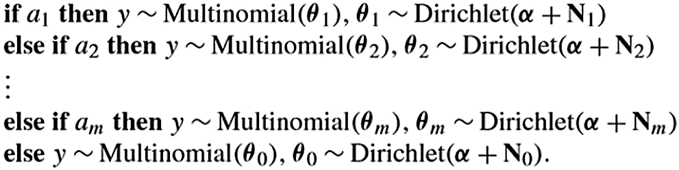
Figure 1: Rule list in distribution format [7]
The Bayesian approach has been proposed for use as a rule mining model [8]. In that study, the authors wanted to identify rare but accurate rules, while mentioning the issue of support. First, they selected candidate rules and checked whether they passed the selection criteria based on Bayesian posterior probability. Second, they combined each rule and checked whether it passed the criteria. The algorithm was executed in a breadth-first approach like the a priori algorithm. The experiment was conducted to find association rules as opposed to classification. As a result, they found two more association rules that could not be found with the support criteria.
The dataset used in this study was a dataset consisting of blood samples of patients infected with COVID-19 that was provided by Yan et al. [3]. There were 75 features, including the personal information of the infected patients and the blood information, which was tested based on date and time. The data consisted of a training data set and a test data set. The training data had 375 patients (201 discharged patients and 174 deceased patients) that were treated from January 10, 2020 to February 18, 2020. The test data had 110 patients (97 discharged patients and 13 deceased patients) that were treated from February 19, 2020 to February 24, 2020 [3]. We filled in the missing values of the training dataset with each feature's mean value. The model was trained using the patient's last day result (death or discharge). The test was conducted 7 days prior to the patient's last day.
As shown in Fig. 2, our proposed model had three stages: feature selection, item generation, and rule extraction. In particular, in rule extraction, we proposed a new rule extraction algorithm that used confidence-closed item mining, JSD, and Bayesian posterior probability. We will define all terminology before explaining the proposed model. Item refers to features relevant to the conditions (e.g., age < 40). Itemset refers to the set of items (e.g., age < 40, sex = female); itemsets refer to multiple itemsets.
Feature extraction involved two tasks. First, we extracted important features by reducing the dependency between features and analyzing the interdependency between the target variable and features. To reduce the dependent features, we used partial correlation, which is a type of correlation that can control the subset of variables with an additional effect; it analyzes the correlation between certain features. Correlation typically indicates the relationship between features without controlling other features. This cannot differentiate between direct and indirect effects [9]. Thus, we used partial correlation to identify more accurate and strict correlation. We calculated the partial correlation between features to remove dependent relations. The partial correlation was calculated using Eq. (1), which can calculate the correlation between x and y when given a single controlling variable z [10]. As we can see in Eq. (1), before we solve this equation, we need to know the zero-order correlation between all possible pairs of variables ((x,y) and (y,z) and (x,z)) [10].
In the feature selection stage, we used the mutual information between the target variable and the features. Mutual information was the probability that event X and Y would occur simultaneously among event X and event Y. If X and Y frequently occur together, it means they have a high interdependency. Features were removed if the mutual information value was below the mutual information threshold. Discrete features were calculated with Eq. (2), while continuous features were calculated with Eq. (3) [11].
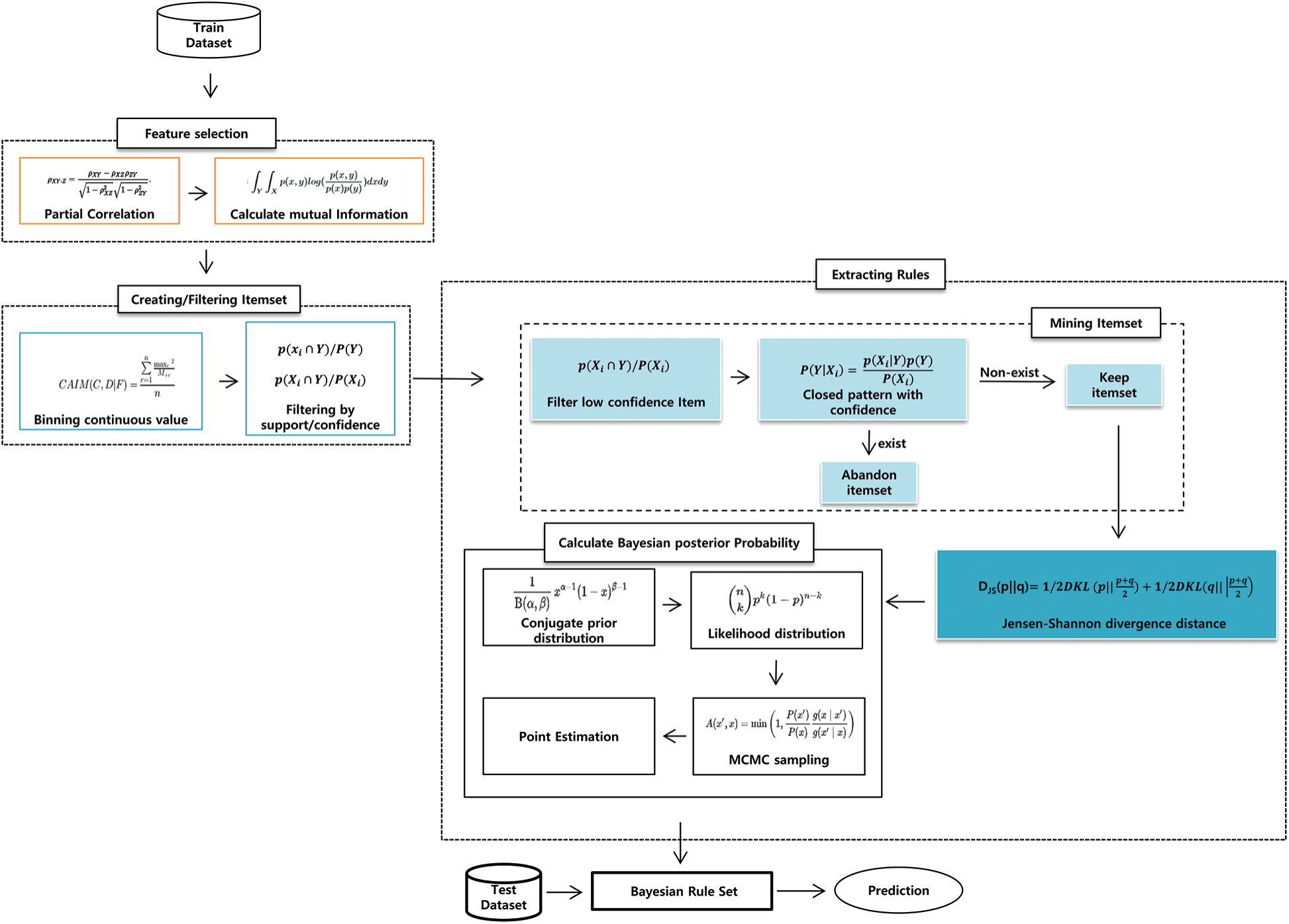
Figure 2: Framework of the proposed model
4.2 Item Generation and Filtering
In the item generation step, the selected features were binned. If the value was smaller than or equal to the split point, it was set to fk ≤ δ; if it was bigger, it was set to δ < fk. We use the Class-Attribute Interdependency Maximization (CAIM) algorithm for binning [12]. The CAIM algorithm is a binning algorithm that can determine the minimal discretization range using the minimal interdependency information loss. The algorithm can discretize the continuous value at the highest CAIM value. The calculation proceeds until reaching the point at which CAIM > Globalcaim or p < k. p means the number of split points and k means the number of classes. CAIM's criteria were defined by Eq. (4). C means the target variable, D means the discretized variable for F, maxr is the maximum value in r range, and N+r is the number of samples in the range [12].
After creating the items, we filtered items with low support and confidence. Due to the a priori nature, we can delete single items with a lower support value than the threshold. However, in the confidence filtering, we can't use priori nature, so we deleted very low confidence items to prevent the creation of a redundant and useless itemset.
4.3 Rule Extraction Using JSD and Posterior Probability
In this stage, the itemset with a high posterior probability was extracted, and rules were generated. The rule extraction consisted of three stages: mining the itemset, filtering with JSD, and filtering with Bayesian posterior probability.
First, we created an itemset with filtering for support and confidence using FP-growth [13] for mining. In the mining process, we filtered the itemset using support and confidence thresholds. Then, we checked if the itemset satisfied the confidence-closed itemset condition.
The confidence-closed itemset is closed itemset, which is focus on confidence. A closed itemset is typically focused on support. If the itemset and superset of the itemset have the same support, then the itemset is removed [14]. However, we focused on confidence instead of support. We deleted the itemset that was the superset of the itemset that had a lower confidence value than the itemset (e.g., {a, b} = 0.8 and {a, b, c} = 0.7, then {a, b, c} was deleted). Since we extracted the ruleset, if the sample matched to itemset({x, y}), then it matched to the superset of itemset({x, y, z}) 100%. However, we could not be certain that the itemset({x, y}) was the correct based solely on confidence. Thus, in this stage, we only deleted the superset with lower confidence, not all of them. Because lower confidence refers to a lower probability of co-occurrence of itemset and Y (e.g., class = 1 in this model), additional items can harm the creation of an effective rule. We checked the condition to avoid creating inaccurate rules and wasting mining time. Using confidence-closed itemset filtering, we could extract an itemset that was less redundant but more accurate.
4.3.2 Itemset Filtering with JSD
In this stage, we calculated the distance between the mined itemsets and the training dataset. We used JSD to calculate the distance. JSD is a variation of Kullback–Leibler (KL), which represents the distance between two distributions. In general, KL refers to the expectation of an information loss value between two distributions. It is used to measure the similarity of two distributions. However, for KL, the differences between the two distributions were not symmetrical. They are not marked as distances, which is equal to Eq. (5) [15]. In this equation, P and Q are the distribution.
The KL between the median of each distribution and the two distributions was performed to make the difference between two distributions symmetrical. This allowed for the distance between the two probability distributions to be calculated. JSD's equation is shown in Eq. (6) [15].
We calculated the distance between the distribution of each itemset and the distribution of the dataset. We made each itemset's multivariate normal distribution using the mean and covariance values of its features. We also made multivariate normal distributions of death (class = 1) and discharged (class = 0)'s using the features of the itemset. Here, we call In for the nth itemset's distribution, D for class 1(death) distribution, S for class 0 (survival) distribution, and Dn for a distance of In. We made our calculation based on Eq. (7).
Since the number of features could affect the distance between distributions, the distance of the death distribution was divided by the sum of the two distributions (death and discharged) in this study. After calculating the distance of each itemset, the itemset was filtered according to the distance threshold. This stage reduced the training time. Because calculating the posterior probability required a lot of time, we filtered the itemset with a long distance.
4.3.3 Itemset Filtering with Posterior Probability
We calculated the Bayesian posterior probability of each itemset and removed them when they did not exceed the threshold. We used this stage to achieve an accurate probability. Without sampling, we obtained the probability from our dataset alone, which can lead to a biased probability. Thus, we created an approximated posterior distribution using a large number of samples, and we used this distribution for explanation and classification.
Posterior probability was calculated by the Bayesian theorem. Since it was a binary classification, the binomial distribution was used as a likelihood distribution. The parameter n was the total occurrence of items while the parameter k was the occurrence of itemsets that resulted in 1(death). The parameter θ was the binomial probability of k. Beta distribution, which was a conjugate distribution, was used for the conjugate prior to distribution [16]. Then, posterior probability could be calculated as follows [17].
Eq. (8) was derived based on the nature of the joint distribution and equation
The denominator is expressed as follows. Eq. (10) is the same as (9). Eq. (11) is derived based on the fact that it becomes 1 if the probability density function of the beta distribution whose parameter is k+α and β+n-k is integrated [17].
Using the denominator Eq. (11) and numerator Eq. (10) calculated above, the probability can be obtained as follows [17].
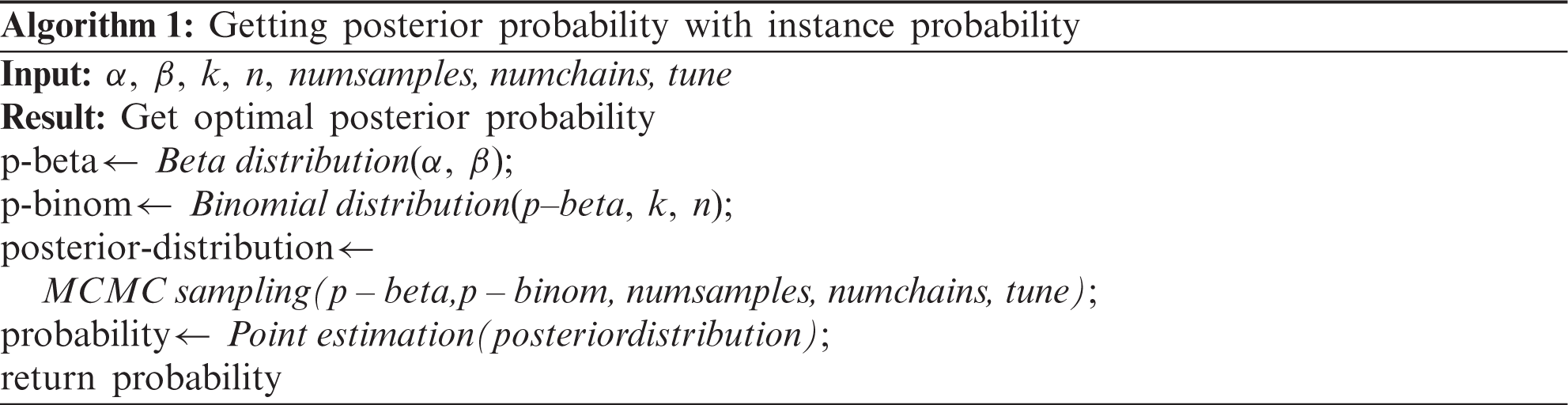
The posterior probability was updated by multiplying the likelihood and the prior probability. Markov chain Monte Carlo (MCMC) sampling was performed to generate an approximated Bayesian posterior probability distribution for each item [18]. The Metropolis-Hastings algorithm was used for sampling. It requires a sampling distribution g(x), which is proportional to the target distribution and the conditional probability distribution q(xt+1|xt), to approximate the target distribution p(x) [19]. The sampling distribution g(x) in this model is the beta-binomial distribution. The process is as follows [19]:
① Pick a distribution g(x) for sampling.
② Choose X0 which is the start point of the Markov chain.
③ Sample y from g(x) which is the candidate of Xt+1 when this chain is X=xt.
④ Calculate the acceptance ratio using Eq. (13).
⑤ Sample u from the uniform distribution U(x) and get Xt+1 using the following process.
⑥ Continue this process (3,4,5) until the stationary distribution appears.
In process 5,
The itemsets were filtered based on the calculated posterior probability. Through this step, the itemsets with high posterior probability were extracted. Since our model was based on a ruleset and we were certain that the itemset was accurate with posterior probability, we filtered the superset of the itemset as described in Section 4.3.1.
The experiment was conducted using a COVID-19 patient blood dataset. The results and threshold values of the proposed model are described here. The threshold values mentioned in this study are determined through several experiments.
First, we deleted features with a dependency value above 0.7, which was our dependency threshold. Next, we deleted features with a value lower than 0.3, which was the mutual information threshold. We then selected 10 features {Lactate dehydrogenase, neutrophils(%), Hypersensitive C-reactive protein, (%)lymphocyte, monocytes(%), procalcitonin, D-dimer, International standard ratio, Amino-terminal brain natriuretic peptide precursor(NT-proBNP), albumin} from the 75 features.
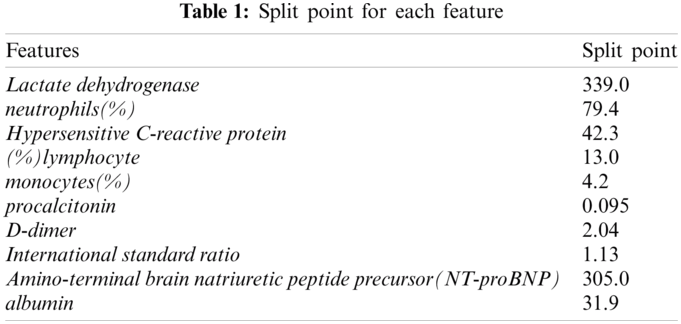
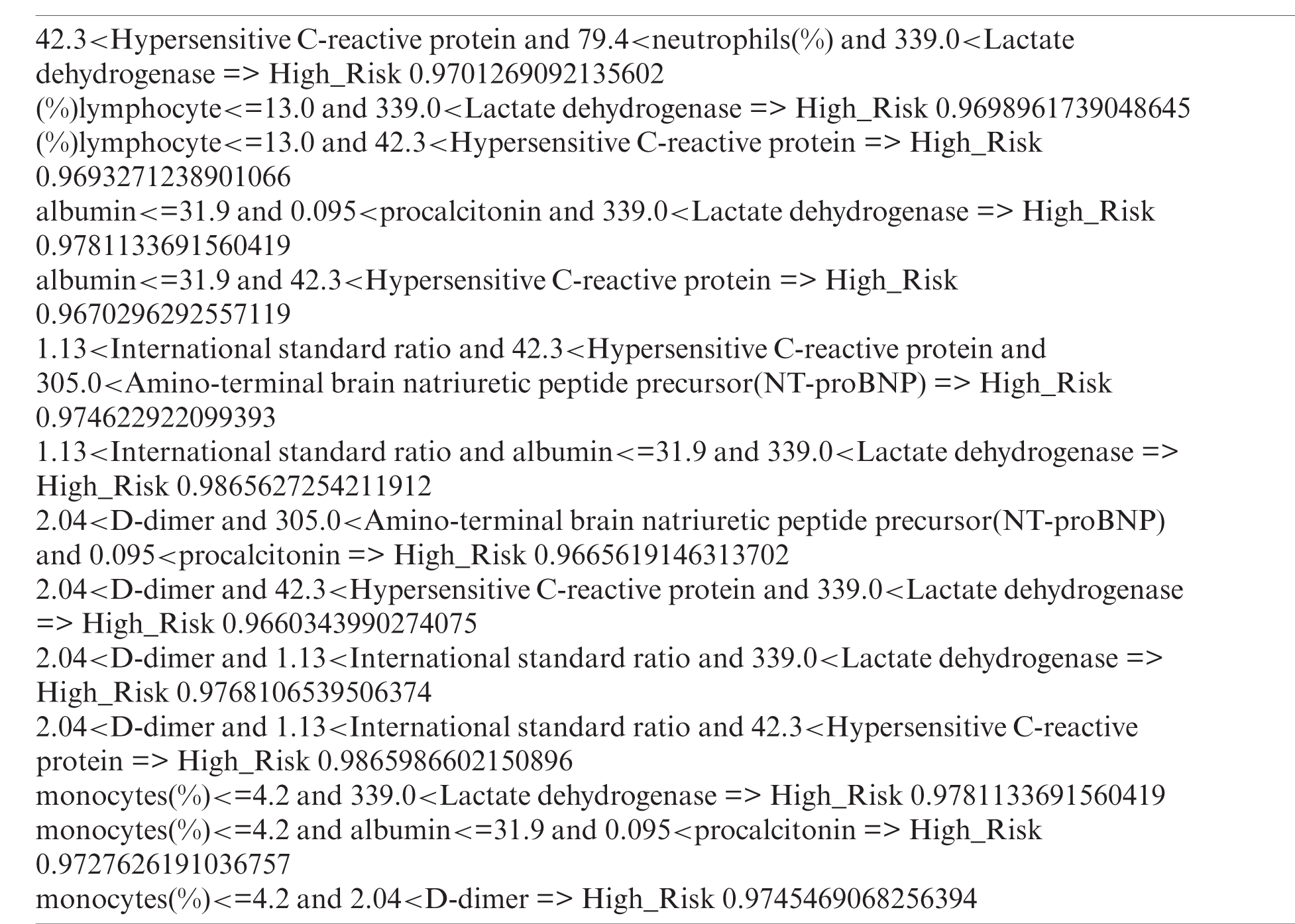
In the item generation step, the continuous features were binned. First, we used the CAIM algorithm [12] to split the continuous values. Tab. 1 lists the split point for each feature.
After creating the items using each split point, we filtered each item using support and confidence thresholds. The support threshold was 0.1 and the confidence threshold was 0.3. After filtering, we extracted a total of 10 items {305.0<Amino-terminal brain natriuretic peptide precursor(NT-proBNP), monocytes(%)<=4.2, (%)lymphocyte<=13.0, 0.095<procalcitonin, 339.0<Lactate dehydrogenase, albumin<=31.9, 1.13<International standard ratio, 2.04<D-dimer, 79.4<neutrophils(%), 42.3<Hypersensitive C-reactive protein}.
5.3 Rule Extraction Using JSD and Posterior Probability
In the mining process, we filtered the itemsets with a support value lower than the support threshold (0.15) and the confidence threshold (0.9). Next, we calculated the distance between the distribution of the itemset and 1(death) or between the distribution of the itemset and 0 (discharged). We deleted the itemset with a distance higher than 0.035. Using JSD, we selected 65 itemsets from 171 itemsets. Fig. 3 shows the distribution of the itemset and class distributions. The left one has a short distance to 1 (death), while the right one has a long distance to 1 (death). The upper one is the itemset distribution, the middle one is the l (death) class distribution, and the bottom one is the 0 (survival) class distribution. As shown in the figure, under short distance conditions, the distributions of itemset and class 1 had similar shapes. The highest conditions and values between them were similar. However, in the long distance condition, the distributions of itemset and class 1 had different shapes and values.
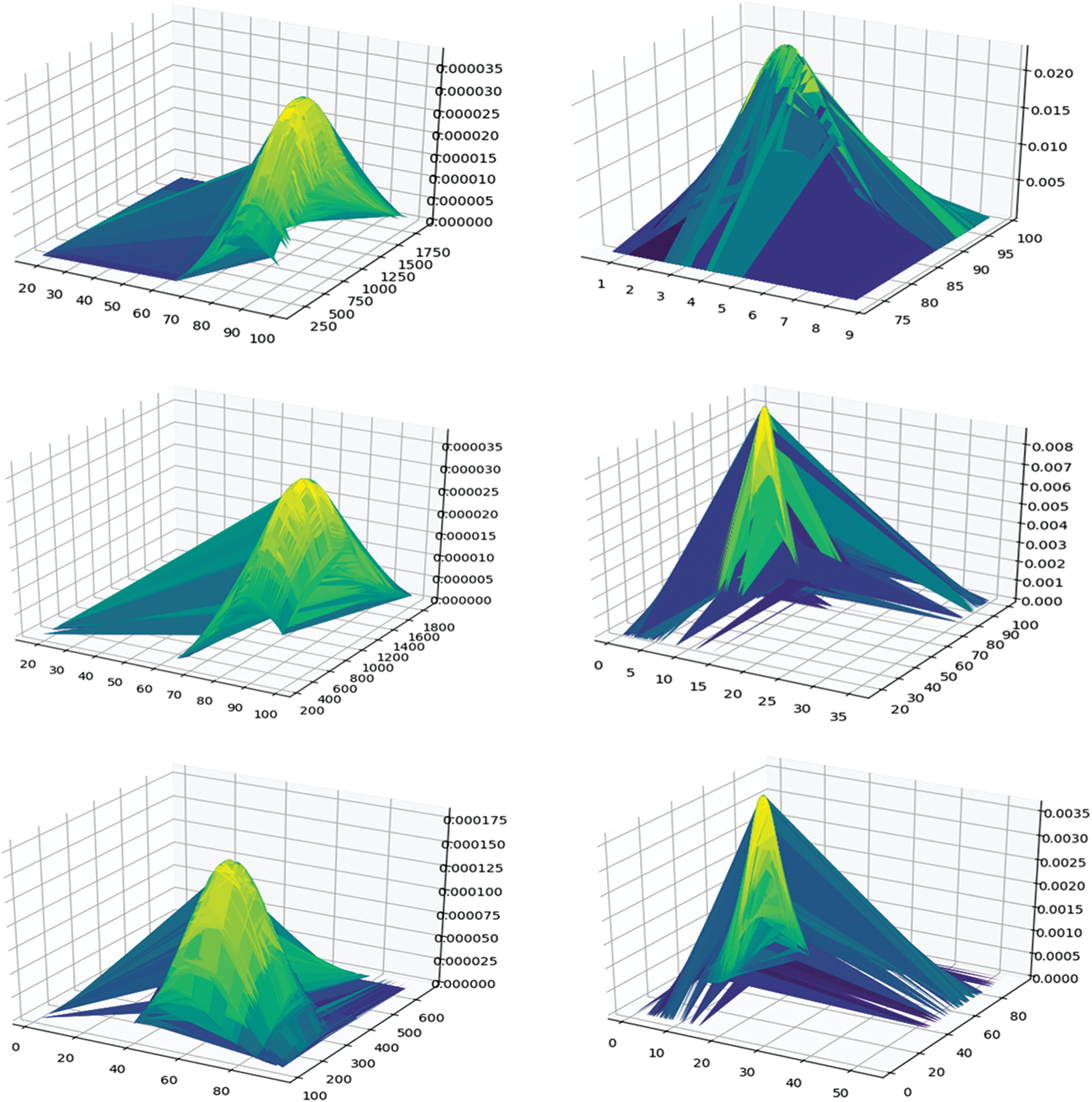
Figure 3: Distribution of itemset, class 1, and class 0
After filtering based on distance, we calculated the Bayesian posterior probability for each filtered itemset. The threshold of each itemset's posterior probability was 0.96. Fig. 4 shows the approximated posterior probability distribution. The upper one had a low probability while the bottom one had a high probability; the left one shows distribution and the right one shows the probability of samples. The highest point was the estimated point.
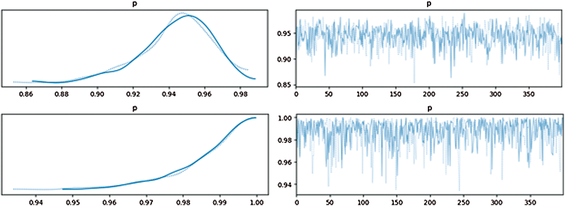
Figure 4: Approximated posterior distribution and probability for samples
Through the Bayesian posterior probability filtering, we selected 20 rules. After the superset filtering, we deleted 6 redundant rules. Therefore, in total, 14 rules were extracted.
We evaluated the performance using the validation data set divided at a 20% ratio; the test data set was provided separately. Since early prediction is important in real situations, the test performance is evaluated using data from 7 days before the result (survival or death) is released. The performance evaluation of the validation dataset was conducted through 100 rounds of five-fold cross-validation for evaluation; we executed our model five times and each fold of the ruleset was performed over 100 rounds. The ROC curve, precision, recall, F1-score, AUC score, and accuracy were used as performance metrics.
Tabs. 2 and 3 present the performances of the XGBoost model, the Fuzzy model, and the proposed model obtained using the validation dataset and the test dataset. The XGBoost model came from [3] and the fuzzy model came from [4]. With the validation dataset, our model had better performance and smaller variance than the XGBoost [3] model. With the test dataset, the proposed model showed the best performance. Thus, overall, our model has good performance and generalization.
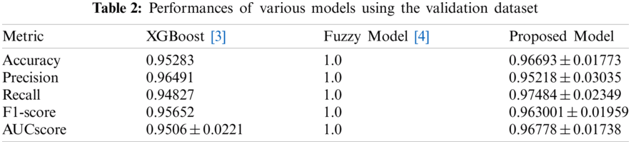
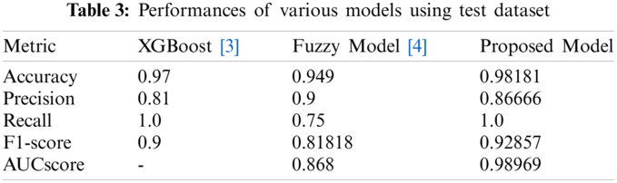
Fig. 5 illustrates the performances of SVM, RandomForest, Gradient Boosting, KNN, and the proposed model using the validation dataset. These figures illustrate performance in terms of box plots. The results show that our proposed model had good performance and very small variance with the validation dataset. Specifically, the performance of our model was similar to or better than that of the blackbox model such as random forest or gradient boosting. Fig. 6 shows the performances of SVM, RandomForest, Gradient Boosting, and KNN obtained with the proposed model using the test dataset. The result show that our proposed model achieved the best performance.
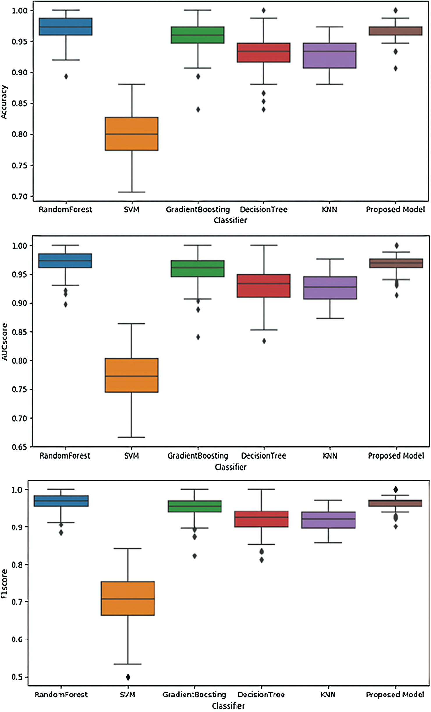
Figure 5: Performances of different models using the validation dataset
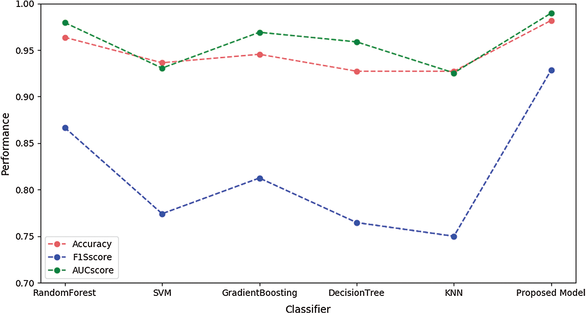
Figure 6: Performances of different models using the test dataset
To separately evaluate the performance of the rule extraction algorithm, we compared the model of the BRL paper [7]. We used our generated item dataset because there was no code for identifying the range of features in the BRL code. Tab. 4 lists the comparison results of the rule extraction using BRL with the validation dataset. Fig. 7 shows the confusion matrix of each model's performance with the test dataset; the left one was from our model and the right one was from BRL [7].
The results revealed that our model showed improved performance, especially with the test dataset. It shows our model has great generality.
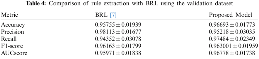
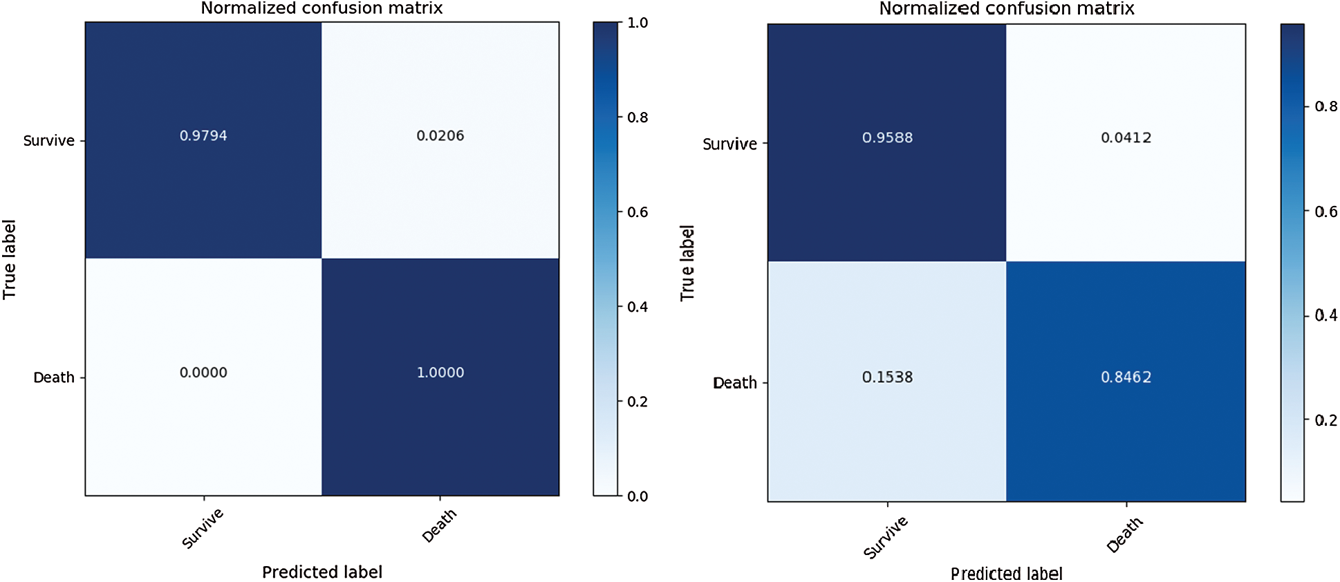
Figure 7: Comparison of rule extraction with BRL using test dataset
The results show that the proposed model has higher accuracy and improved interpretability. It provides posterior probability with rules. It gives a good explanation for why it makes the predictions it does and that can lead to user reliability. Further, it provides various insights; for one, it provides the probability agrees with the argument that probability modeling is important in clinical practice [21]. The model shows great performance in 100-round five-fold cross-validation with the test and validation dataset, thus demonstrating high accuracy and generality. In other words, this model addressed the trade-off problem between interpretability and accuracy using blood samples of patients infected with COVID-19. Future research should focus on applications and improving the model. To strengthen its application in real situations, we will perform experiments with our model using various medical datasets to achieve high generalizability and interpretability. To improve the model, we will optimize the model to find the optimal threshold; this proposed model chooses the optimal thresholds based on the results of multiple experiments. This method does not have an optimal value, and it takes a lot of time. To solve this problem, we study optimization algorithms such as the genetic algorithm [22] and Bayesian optimization [23] to find the optimal threshold.
Acknowledgement: Thanks my mother, leading professor with lab colleague, my friends and my cats for endless support.
Funding Statement: This research was supported by the MSIT (Ministry of Science and ICT), Korea, under the ITRC (Information Technology Research Center) support program (IITP-2021–2020–0–01602) supervised by the IITP (Institute for Information & Communications Technology Planning & Evaluation).
Conflicts of Interest: The authors declare that they have no conflicts of interest to report regarding the present study.
1. World Health Organization (WHO“Coronavirus disease (COVID-19) pandemic, number at a glance,” 2020. Retrieved from https://www.who.int/emergencies/diseases/novel-coronavirus-2019. [Google Scholar]
2. World Health Organization (WHO“COVID-19 severity,” 2020. Retrieved from https://www.who.int/westernpacific/emergencies/covid-19/information/severity. [Google Scholar]
3. L. Yan, H. T. Zhang, J. Goncalves, Y. Xiao, M. Wang et al. “An interpretable mortality prediction model for COVID-19 patients,” Nature Machine Intelligence, vol. 2, no. 5, pp. 1–6, 2020. [Google Scholar]
4. P. Gemmar, “An interpretable mortality prediction model for covid-19 patients-alternative approach”, MedRxiv, 2020. [Google Scholar]
5. L. Zhang, X. Yan, Q. Fan, H. Liu, X. Liu et al. “D-dimer levels on admission to predict in-hospital mortality in patients with covid-19,” Journal of Thrombosis and Haemostasis, vol. 18, no. 6, pp. 1324–1329, 2020. [Google Scholar]
6. L. Tan, Q. Wang, D. Zhang, J. Ding, Q. Huang et al. “Lymphopenia predicts disease severity of COVID-19: A descriptive and predictive study,” Signal Transduction and Targeted Therapy, vol. 5, no. 1, pp. 1–3, 2020. [Google Scholar]
7. B. Letham, C. Rudin, T. H. McCormick and D. Madigan, “Interpretable classifiers using rules and Bayesian analysis: Building a better stroke prediction model,” The Annals of Applied Statistics, vol. 9, no. 3, pp. 1350–1371, 2015. [Google Scholar]
8. L. I. L. González, A. Derungs and O. Amft, “A Bayesian approach to rule mining,” arXiv preprint, arXiv:1912.06432, 2019. [Google Scholar]
9. L. Nie, X. Yang, P. M. Matthews, Z. Xu and Y. Guo, “Minimum partial correlation: An accurate and parameter-free measure of functional connectivity in fMRI,” Int. Conf. on Brain Informatics and Health, vol. 9250, pp. 125–134, 2015. [Google Scholar]
10. H. Griffin, “A further simplification of the multiple and partial correlation process,” Psychometrika, vol. 1, no. 3, pp. 219–228, 1936. [Google Scholar]
11. T. M. Cover, “Introduction and preview,” in Elements of Information Theory 2nd ed., Hoboken, New Jersey, USA: John Wiley & Sons, pp. 1–13, 1999. [Google Scholar]
12. L. A. Kurgan and K. J. Cios, “CAIM discretization algorithm,” IEEE Transactions on Knowledge and Data Engineering, vol. 16, no. 2, pp. 145–153, 2004. [Google Scholar]
13. J. Han, J. Pei and Y. Yin, “Mining frequent patterns without candidate generation,” ACM Sigmod Record, vol. 29, no. 2, pp. 1–12, 2000. [Google Scholar]
14. C. C. Aggarwal, M. A. Bhuiyan and M. A. Hasan, “Frequent pattern mining algorithms: a survey,” in Frequent Pattern Mining, Springer, Cham, pp. 19–64, 2014. [Google Scholar]
15. F. Nielsen, “On the jensen–Shannon symmetrization of distances relying on abstract means,” Entropy, vol. 21, no. 5, pp. 485, 2019. [Google Scholar]
16. C. Forbes, M. Evans, N. Hastings and B. Peacock, “Beta Distribution,” in Statistical Distributions, 4th ed., Hoboken, New Jersey, USA: John Wiley & Sons, pp. 55–61, 2011. [Google Scholar]
17. M. K. Cowles, “Introduction to One-Parameter Models: Estimating a Population Proportion,” in Applied Bayesian statistics: With R and OpenBUGS examples, 1st ed., vol. 98, Berlin/Heidelberg, Germany: Springer Science & Business Media, pp. 25–46, 2013. [Google Scholar]
18. A. E. Gelfand and A. F. M. Smith, “Sampling-based approaches to calculating marginal densities,” Journal of the American Statistical Association, vol. 85, no. 410, pp. 398–409, 1990. [Google Scholar]
19. C. Andrieu, N. D. Freitas, A. Doucet and M. I. Jordan, “An introduction to MCMC for machine learning,” Machine Learning, vol. 50, no. 1, pp. 5–43, 2003. [Google Scholar]
20. C. P. Robert, “Bayesian point estimation,” in the Bayesian Choice, Springer, New York, NY, Springer Texts in Statistics, pp. 137–177, 1994. [Google Scholar]
21. R. Bellazzi and B. Zupan, “Predictive data mining in clinical medicine: Current issues and guidelines,” International Journal of Medical Informatics, vol. 77, no. 2, pp. 81–97, 2008. [Google Scholar]
22. K. F. Man, K. S. Tang and S. Kwong, “Genetic algorithms: Concepts and applications [in engineering design],” IEEE Transactions on Industrial Electronics, vol. 43, no. 5, pp. 519–534, 1996. [Google Scholar]
23. M. Pelikan, D. E. Goldberg and E. Cantú-Paz. “BOA: The Bayesian optimization algorithm,” Proc. of the Genetic and Evolutionary Computation Conf. GECCO-vol. 99, no. 1, pp. 525–532, 1999. [Google Scholar]
 | This work is licensed under a Creative Commons Attribution 4.0 International License, which permits unrestricted use, distribution, and reproduction in any medium, provided the original work is properly cited. |