Computers, Materials & Continua DOI:10.32604/cmc.2021.017710
Article

A Compromise Programming to Task Assignment Problem in Software Development Project

Ngo Tung Son1,2,*, Jafreezal Jaafar1, Izzatdin Abdul Aziz1, Bui Ngoc Anh2, Hoang Duc Binh2 and Muhammad Umar Aftab3

1Department of Computer and Information Sciences, Universiti Teknologi Petronas, Seri Iskandar, 32610, Malaysia
2Department of Information and Communication Technology, FPT University, Hanoi, 100000, Vietnam
3Department of Computer Science, National University of Computer and Emerging Sciences, Chiniot-Faisalabad Campus, Chiniot, 35400, Pakistan.
*Corresponding Author: Ngo Tung Son. Email: sonnt69@fe.edu.vn
Received: 08 February 2021; Accepted: 29 April 2021

Abstract: The scheduling process that aims to assign tasks to members is a difficult job in project management. It plays a prerequisite role in determining the project’s quality and sometimes winning the bidding process. This study aims to propose an approach based on multi-objective combinatorial optimization to do this automatically. The generated schedule directs the project to be completed with the shortest critical path, at the minimum cost, while maintaining its quality. There are several real-world business constraints related to human resources, the similarity of the tasks added to the optimization model, and the literature’s traditional rules. To support the decision-maker to evaluate different decision strategies, we use compromise programming to transform multi-objective optimization (MOP) into a single-objective problem. We designed a genetic algorithm scheme to solve the transformed problem. The proposed method allows the incorporation of the model as a navigator for search agents in the optimal solution search process by transferring the objective function to the agents’ fitness function. The optimizer can effectively find compromise solutions even if the user may or may not assign a priority to particular objectives. These are achieved through a combination of non-preference and preference approaches. The experimental results show that the proposed method worked well on the tested dataset.

Keywords: Makespan; RCPSP; scheduling; MOP; combinatorial optimization; compromise programming; genetic algorithm;

1  Introduction

1.1 Research Context

In software project management, scheduling plays a critical role in the success of a project. Scheduling starts with the work breakdown structure (WBS), which allows the whole project to be broken down into smaller tasks, which are assigned to project team members based on their skills and knowledge according to the working plan. In reality, projects run under constraints, including those of human resources, budget, and time. The lack of a helpful management toolset makes it difficult to achieve the goals of the shortest critical path, lowest cost, and highest quality. We develop an approach based on a multiobjective optimization model and a metaheuristic algorithm that generates an optimal project schedule to meet the above goals. Fig. 1 depicts the scheduler, which takes a list of tasks, project team members’ profiles, and decision-makers’ preferences as the model’s inputs. The output is a detailed schedule. The time to complete a project depends on the available time, the similarity of tasks, and their interdependence. These factors also affect the cost and quality of the project.

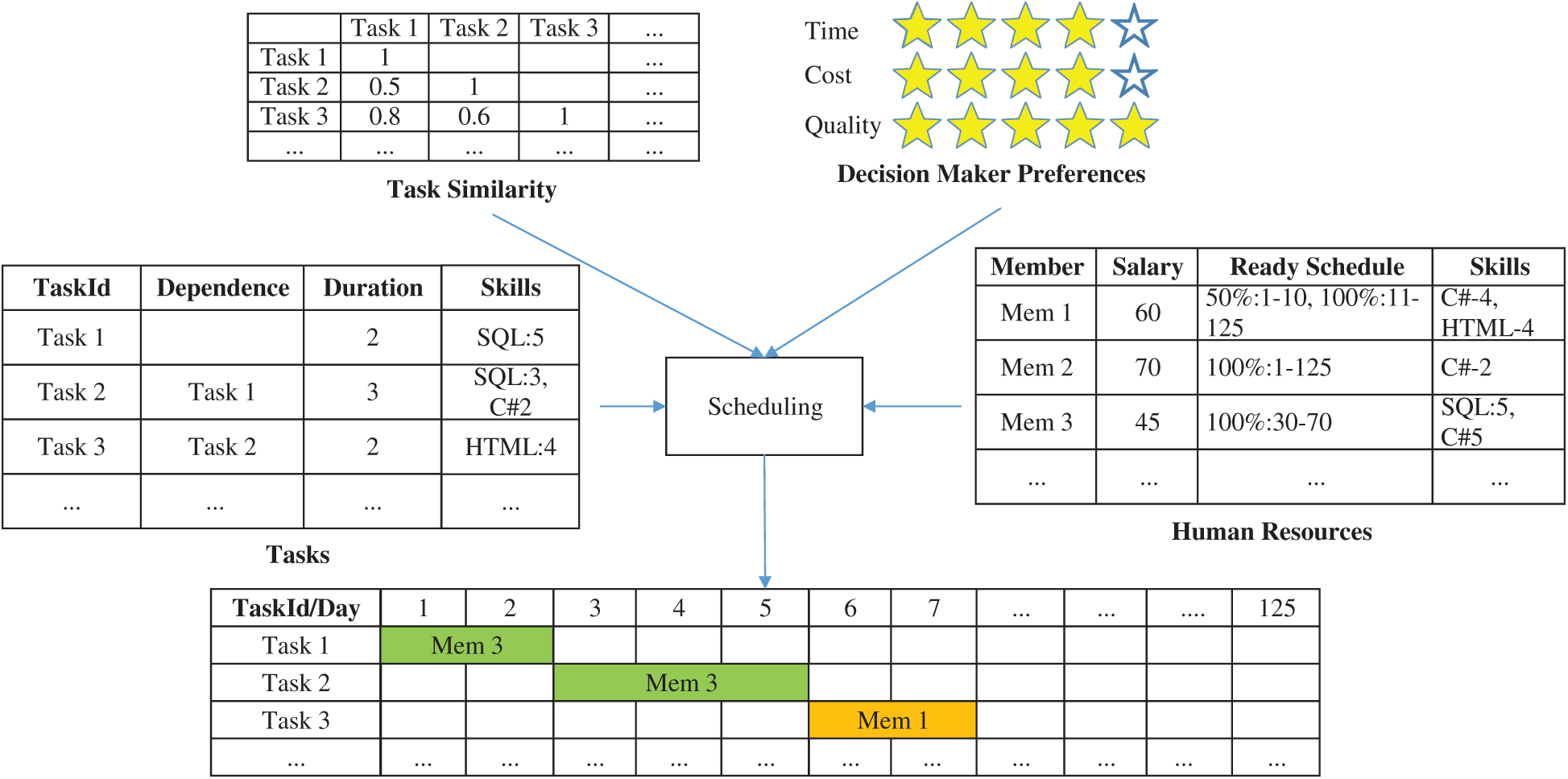
Figure 1: Process of assigning tasks to each member of a project

1.2 Related Researches

Scheduling problems that deal with workforce constraints have the form of a resource-constrained project scheduling problem (RCPSP) [1–5]. Habibi et al. classified many RCPSP problem variations and mentioned modeling and algorithms to find optimal solutions for this type of problem in a 2018 survey [6]. Vanhoucke and Coelho presented an overview of state-of-the-art RCPSP algorithms [7]. The situation described in the first section of this paper is a multiobjective problem [8]. A primary objective is to solve the makespan problem, i.e., to complete the project in the shortest duration [9]. Makespan scheduling is described as follows: Assume M machines and N jobs for scheduling, where the nth job takes pn,m units of time if scheduled on the mth machine. Let Jm be the set of jobs on the mth machine; then the machine’s load is lm=∑j∈Jmpj,m. The maximum load is lmax=maxm=1,…,Mlm. Let xn,m be the decision variable to determine the nth job assigned to the mth machine. The minimum makespan becomes min(f), subject to: ∑m=1Mxn,m=1 ∀n=1,2,…,N, ∑n=1Npn,m∗xn,m≤f ∀m=1,…,M, and xn,m∈{0,1} ∀n=1,…,N,m=1,…,M.

The interdependence of tasks often is expressed as a directed graph. Two fake tasks, the head (task 0) and tail (task N + 1), of zero duration, are added to formulate a single started/ended graph, as shown in Fig. 2. The makespan is now computed by any traversal method, such as breadth-first search (BFS). As mentioned in Section 1.1, the makespan may be affected in several ways. The tasks’ interdependence determines the best critical path by the longest path in the graph. This constraint combines with the personnel’s sequential workload, and their schedules may increase the critical path’s length.

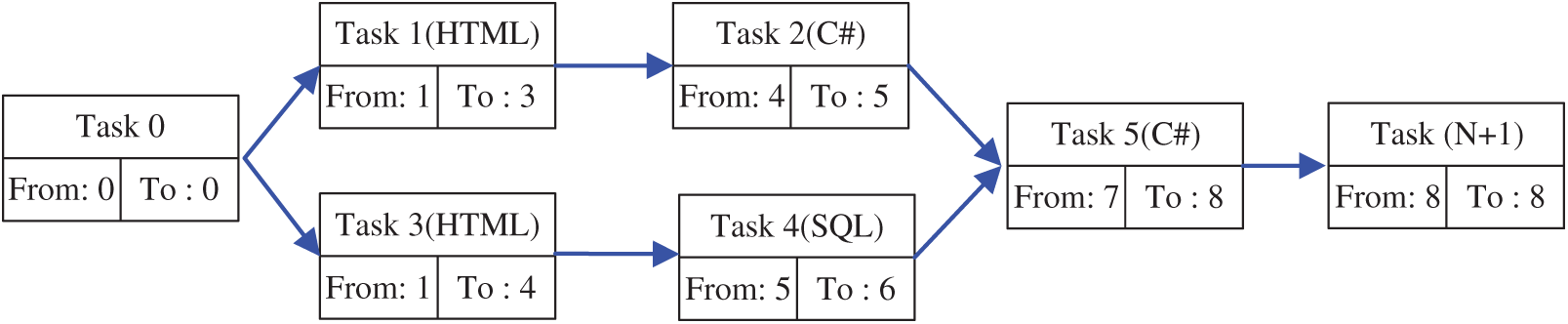
Figure 2: Head and tail tasks added to PERT chart to transform the problem to a single-start, single-end problem

Among recent studies on RCPSP and its variants Kumar et al. [10] proposed an algorithm to solve the classical RCPSP and minimize the makespan. Arian [11] designed an evolution algorithm to solve RCPSP, with the objective to minimize project cost, using binary decision variables to represent the time-unit when the activities started. Laurent et al. [12] and Stiti et al. [13] introduced a variant of multiside RCPSP, considering mobile and fixed resources in the transportation system. A variant of RCPSP subjected the project to renewable resources, each available for limited periods during the project life cycle, and applied a penalty cost for keeping resources for extra periods [14]. Quoc et al. [15] introduced Real-RCPSP, a variant of MS-RCPSP, and {R-CSM}, an algorithm to solve it based on cuckoo search. Hosseinian et al. [16] tried to maximize modularity to find high-quality employee communities and arrange them for tasks based on them. Nadjafi [17] proposed a mixed-integer programming formulation of RCPSP to minimize the total project cost, considering earliness-tardiness and preemption penalties. Ahmadpour et al. [18] presented a model of RCPSP by viewing a working calendar for project members and determining the skill factor of any member using the efficiency concept. Kellenbrink et al. [19] introduced two subproblems of RCPSP, the first to select activities, and the second to minimize makespan and total cost. Joshi et al. introduced a model to minimize the makespan or entire project duration. The objective was subject to activities’ resource requirements at some finite integer value other than 1. The resources were staff members mastering one or more skills [20]. Tesch et al. [21] developed a mixed-integer programming formulation for RCPSP, improving the optimal problem-solving method over the previous approach by investigating relationships between event-based and time-indexed models.

Many other issues can arise in real-world situations, such as the division of labor in an organization, members’ concentration in different project phases, and similarities of tasks. Project managers often assume that if a worker is assigned many similar tasks, then the job’s cost will increase or decrease [22]. As in other engineering disciplines, to reuse previous work is critical to the progress and quality of software projects. In short, the more similar things a worker does the lower the cost. These aspects affect the objectives of project management.

RCPSP is combinatory optimization [23], and algorithms may not exist to find the optimal solution in polynomial time. In this case, metaheuristics have proved efficient in many case studies [24]. Tao et al. [25] introduced a procedure based on simulated annealing. Zhang et al. [26] designed a genetic algorithm with renewable resources and a single mode to perform each activity. Van et al. [27] introduced a genetic algorithm (GA) to solve both multimode and preemptive multimode RCPSP. However, most of these studies are in the form of problem-algorithm-result, and are not applicable to the proposed problem due to different business requirements. Based on results of previous studies, we construct a multiple-objective optimized mathematical model. Human resources, including skills, available time, salary, and task similarity, are constrained, in addition to constraints such as budget and deadline. We design a genetic algorithm to solve the model.

1.3 Contributions

In this research, we designed a new multi-objective optimization model for RCPSP problems that applies to software development in addition to our case study. It may be helpful in other task scheduling and project management work. Our model generates a detailed project schedule. The aim is to complete a project with the shortest duration while maintaining quality at a reasonable cost. It expresses the significant considerations of the decision-makers in the planning process. The model introduces some new rules related to human resources essential to software project management (and other engineering areas). We combine the preferred and non-preference approaches to transform the multi objective problem to a single-objective problem. Both methods have advantages and disadvantages and are suitable for different decision-makers. They are combined to leverage their benefits and cover each other’s drawbacks. Section 2 of this paper describes the model.

The second contribution is to propose a new GA to solve the model. Unlike the usual mathematical programming or heuristic approach, the proposed method allows incorporation of the MOP approach in the algorithm design. To guide individuals in the search process, we use a distance-based objective function as their fitness. Section 3 describes the algorithm’s implementation. The experimental procedure on the real dataset and its results are discussed in Section 4. We relate our conclusions in Section 5. Researchers in scheduling, planning, project administration, operations, and management can benefit from this research.

2  Multi-Objective Optimization Model

2.1 Problem Formulation

We define some frequently used variables:

•   N is a number of tasks.

•   dnbegin and dnend are respectively the expected start and end dates of the nth task.

•   S is the number of required skills for the project.

•   M is the number of candidates.

•   A={Ai,j∣Ai,j∈{0,1} i=0,…,N+1,j=0,…,(N+1)} is the adjacency matrix of the directed-weighted graph that represents the dependences of the tasks. The 0th and (n+1)th nodes are fake nodes added as the head and tail, where d0end=d0begin,dn+1end=dn+1begin.

•   K={Km,s∣Km,s∈{0,1,…,5},m=1,…,M,s=1,…,S}, where Km,s≥1 if the mth candidate has the sth skill; a greater value of Km,s indicates that the mth member has more experience with the sth skill, and Km,s=0 means the mth member has no experience with the sth skill.

•   R={Rn,s∣Rn,s∈R+,n=1,…,N,s=1,…,S}, where Rn,s is the required level of the sth skill. Rn,s and Km,s are bounded by the same range of values.

•   fnbegin and fnend are the actual start and end times, respectively, of the nth task when assigned to a member.

•   Tm is the cost to hire the mth member to work for one time unit.

•   Z={zi,j∣zi,j∈[0,1],i=1,…,N,j=1,…,N} is the similarity matrix of the tasks, where zi,j is the similarity between the ith and jth tasks.

•   D is the project deadline.

•   U={um,d∣um,d∈[0,1],u=1,…,M,d=1,…,D} describes the concentration of personnel in a given time period; e.g., um,d=0.5 means the mth member only attends 50% at time unit d.

•   B is the project budget.

•   Decision variables: X={xn,m∣xn,m∈{0,1},n=1,…,N,m=1,…,M} , where xn,m=1 if the nth task is assigned to the mth member, and xn,m=0 otherwise.

The project has three objectives:

•   Minimize the critical path/makespan:

min(g1(X)=fn+1end) (1)

Factors such as the concentration of members and similarity between tasks affect the time to complete the task.

•   Minimize the cost of hiring team members:

min(g2(X)=∑m=1M(∑d=minn=1,…,N(xn,m∗fnbegin)maxn=1,…,N(xn,m∗fnend)(um,d∗Tm))) (2)

•   Maximize the experience of selected candidates. Experience dramatically affects the quality of the project. The more experienced the candidate the less likely are errors:

max(∑n=1N∑m=1M∑s=1Sxn,m∗Km,s)=min(g3(X)=−1∗∑n=1N∑m=1M∑s=1Sxn,m∗Km,s), (3)

subject to:

•   All tasks are assigned to members:

∑n=1N∑m=1Mxn,m=N (4)

•   A task is assigned to only one member:

∑m=1Mxn,m=1∀n=1,…,N (5)

•   A member does not simultaneously perform two tasks:

∀m=1,…,M,a=1,…,(N−1),b=(a+1),…,N (6)

•   Dependent tasks cannot be executed at the same time:

Ai,j∗fjbegin−Ai,j∗(fiend+1)≥0∀i=1,…,N−1,j=i+1,…,N (7)

•   A task is assigned to the only member who qualifies:

Rn,s≤xn,m∗Km,s∀n=1,…,N,m=1,…,M,s=1,…,S (8)

•   The project ends on time:

fn+1end≤D (9)

•   Costs do not exceed the budget:

∑n=1N∑m=1M∑s=1Sxn,m∗Km,s≤B (10)

2.2 Approach for MOP

Ignizio said there is no one best approach to all types of multiobjective mathematical programming problems [28]. Solutions to multiobjective optimization problems (MOPs) are categorized as either preference or non-preference [29]. The first approach is to use preference information archived by interviewing the decision-maker to determine the solution that best satisfies these preferences. The second approach assumes that no decision-maker was available, and that we can identify a compromise solution without preference information. Decision-makers often cannot determine priorities, which leads them to try many parameters and select one of several solutions. It is challenging in practice to define meaningful ranges of parameters. The computational cost of a search algorithm is a barrier to finding appropriate parameter values to determine a final solution. Compromise programming allows a one-shot solution.

Compromise programming can solve the above problem by identifying an ideal solution [30] as a point of reference and finding a solution as close as possible to the ideal point. Ngo et al. [31] applied it to their MOP, introducing the concepts of “deep” and “wide” to access the skills of candidate teams. Xiong et al. [32] proposed two levels of compromise programming to allocate resources between pavement and bridge deck maintenance. Poff et al. [33] used compromise programming to represent 20 objective functions to determine the preferred decision variable value and assign a closeness level to an ideal solution. Ngo et al. [34] introduced CP as the difference between the perfect and actual points to solve a multiobjective timetabling problem, and tried to answer strategic questions as decision-makers in simple terms. In such a situation, we answer three questions, and we believe a decision-maker would do the same. What is the earliest time the project can be completed? The shorter the better. What is the lowest cost? The lower the better. At what level should the project quality be? The higher the better.

The answers above can represent the decision-maker’s aspirations when unable to define any preferred objectives.

E={Ei∣i=1,…,3} denotes the expected point, where E=[dn+1end,0,∑n=1N∑m=1M∑s=1SKm,s]

O={Oi∣i=1,…,3} represents the actual solution, where

Instead of maintaining the three goals of the original MOP, we have just the goal to find the point O closest to E. Compromise programming allows us to use any distance function. We select the Euclidean distance to build a new objective function,

Many situations can occur during project planning. We need to assign a priority to each goal. The considered problem has three targets, which can be graphically visualized to better realize the effects of strategies. This is hard to achieve with compromise programming, although it is straightforward to explain that the decision-maker wants to balance goals. Another approach is to scalarize a MOP, i.e., to formulate a single-objective optimization problem whose solutions are Pareto optimal solutions to the MOP. The original multiobjective functions are scalarized and written as min(∑i=13wi∗gi(X)), where wi is the weight of the ith objective function. We want to reuse the good features of compromise programming and linear scalarizing, so we combine the approaches. The distance function’s size is influenced by spatial dimensions [35], and can be manipulated using dimensional weights. The objective function becomes

minimize(distance(E,O))=∑i=13wi∗norm((Ei−Oi)2) (11)

where the norm function normalizes the features of the distance function to the same range.

3  Proposed Algorithm

3.1 Introduction to Genetic Algorithm

Evolutionary algorithms (EA) are mainstream stochastic methods for MOP [36]. In the family of EA, genetic algorithms (GA) are popular choices for engineering applications [37]. It starts searching for the optimal solutions in solution space by forming a population/set of possible solutions. Then new solutions are created by breeding the best fitness individual from the population to generate the new generation. Over the iterations, the population retains the best genetic hybridization combined with mutations to create a better next generation. GA gives a guideline for solving the problem. However, each issue needs a different scheme design. In this study, we introduce a version of the GA to solve the MOP model.

3.2 GA Scheme

Denote:

•   U is population size.

•   G denotes the convergence condition.

•   P(g)={Pi(g),P2(g),…,PU(g)} denotes population.

•   Pi(g)={Pi,1(g),Pi,2(g),…,Pi,N(g)} is an individual of the population.

where: Pi,e(g)=m∈Me

•   Me represents the set of members who able to do a task eth.

•   Our proposed genetic algorithm’s scheme described as following:

•   Initialize g=1

•   timesti is the time that a member ith start the first task;

•   timefni is the time that a member ith complete the last task;

The Genetic Algorithms expressed in 6 steps as follows:

Step 1: Randomly generate the Pi(g) ∀ i=1,2,…,U.

Step 2: Compute fitness value corresponding to Pi(g) ∀ i=1,2,…,U as following:

Step 2.1: Update fnstart, fnend, timestm and timefnm using BFS on matrix A and population Pi(g).

The needed duration to complete a task nth affected by the task similarity, effort distribution of the assigned member. The fnend can be computed as:

where: actual(n,m) is the estimated effort to complete a task nth by member mth. The actual defined as follow.

Step 2.2: Define cost, Mtime, Mcost, Mquality as following.

•   cost=(∑m=1MTm∗(timefnm−timestm))

•   Mtime=∑e=1N(deend−destart)

•   Mcost=maxe=1,…,MTe∗Mtime

•   Mquality=∑e=1N∑x=1S(Re,x∗max(Kz,x)) ∀z=1,…,M.

Step 2.3: The fitness values Pi(g).fitness could be biased due to the difference in ranges of its dimensions. We normalize features to the range [0, 1]. The distance function (11) is rewrite in form of fitness of the individual as:

Step 2.4: Sort the P(g) order by Pi(g).fitness ascending.

Step 3: Elitism Selection: keep an individual b=argmini=1,…,UPi(g).fitness that returns the best fitness for next-generation. Denote the best fitness value of the gth generation as bg. The first individual of the next generation created as: P(g+1).add(Pb(g)).

Step 4: Crossover and mutation: Denote w as the mutation rate. Denote σ as tournament size selection.

For each i=2,…,U.

Step 4.1: Create 2 new populations with a size of σrespectively:

and

where:

rand(PG) is the function that return an item from the input list PG. The returned item is not duplicated with the previous ones.

Step 4.2: Create best genes from P(g),dad and P(g),mom to generate the next generation.

Set r=rand([0,1])

where:

rand([0,1]) returns a float number in range [0,1].

rand(ddad,j,dmom,j)returns ddad,j or ddad,j randomly.

rand(j) randomly returns a value corresponding to a cell jth of a choronosome.

Step 5: Constraint validation checking: if there is an individual Pi(g+1) that violates any constraints defined in Eqs. (4)–(10), then it is removed from the set of results.

Step 6: Return to Step 2 with g=g+1 until bg=bg−1=…=bg−G.

4  Experiments

We validated the proposed method with the real datasets obtained after the WBS process of a software project. The results show that the algorithm works well with the tested dataset. It consisted of 417 dependent tasks, 19 candidates of project members, and 27 required skills. The algorithm was implemented in Java-8 and executed on a computer with an Intel Core I5-8250U CPU @1.60 GHz, with 4 GB RAM. It is essential to find appropriate values for parameters when implementing a GA, as this affects the results. There are many methods to find the best set of parameters. We tried many parameter sets at different ranges to tune the algorithm, and selected w = 0.1, σ = 30, and U = 110, based on the minimum returned fitness values. We temporarily set G to reach 500 generations. To determine how job similarity affects completion time, we consulted experienced engineers and defined:

GA does not guarantee an optimum global result, as the results vary by the initialization. We sought the best result, so we ran the algorithm with the best set of parameters. Results of 15 executions with various initialization values are shown in Tab. 1. The fitness value is affected by three criteria, each with a different range of values. To avoid bias between different target values when calculating E and O distance, we normalized all data on dimensions that are not simple in the range [0, 1]. We could retrieve the same fitness value, but the objective functions returned different values. The execution time ranged from 1 to 1.5 min. Fig. 3 displays the fitness values Pi(g).fitness and corresponding objective functions defined in Eqs. (1)–(3) as they changed over generations. We can observe that fitness values always decrease over generations because the selection always keeps the individual with the best fitness. The objective function’s values can be incremented or decremented at a given generation when the fitness value between them does not change.

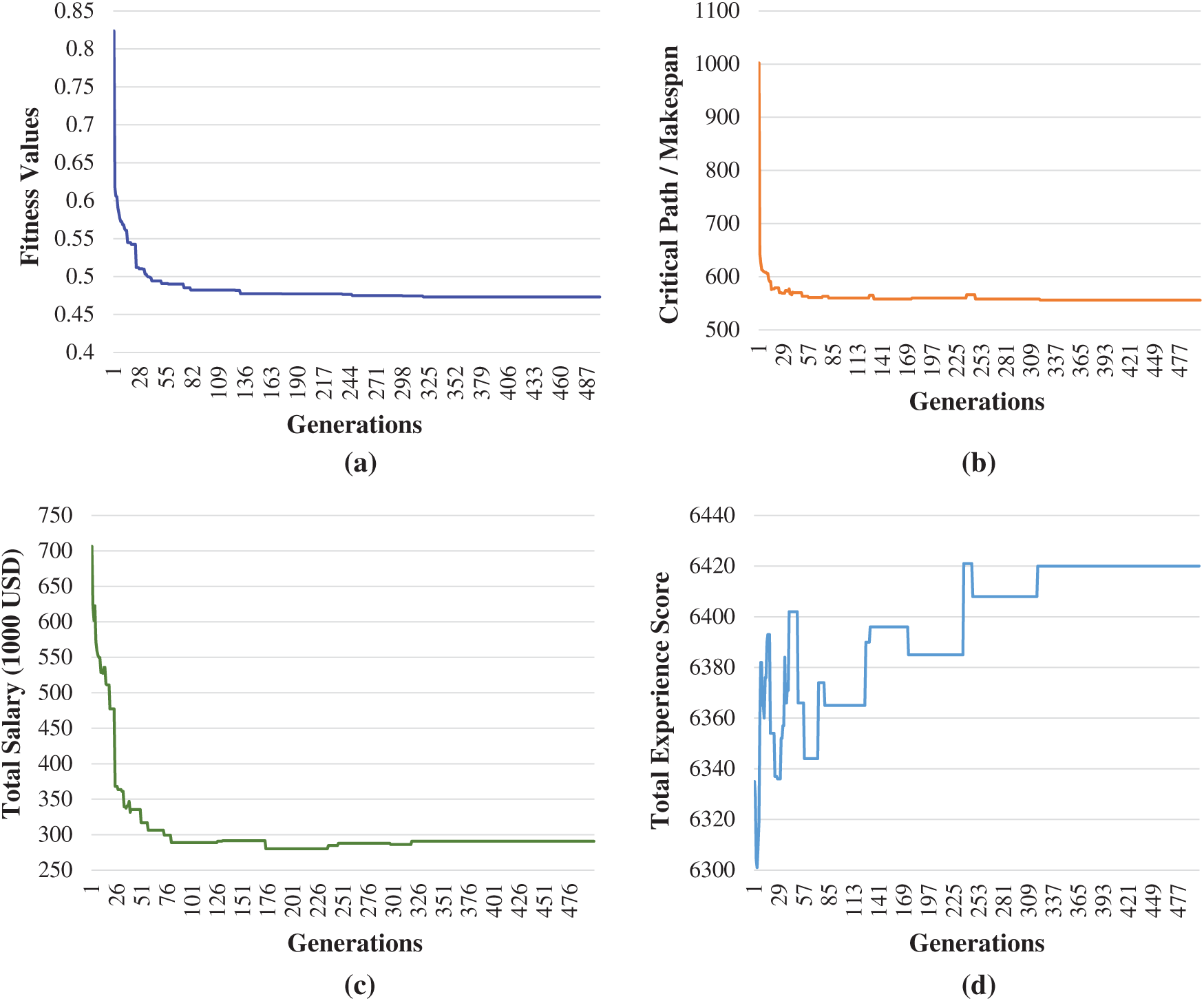
Figure 3: (a) Fitness values (b) Critical path objective values, (c) Total salary objective values, (d) Total experience score objective values; changing over generations

A schedule for each candidate for each time unit is shown in Fig. 4. A line represents a candidate, and columns represent the units of times. Assigned jobs have colors different from the background. We can notice that some members were used for a long time, while most were used occasionally. We checked with data on the availability of members. Members 3, 16, and 20 are those with the most registered time on the project, which explains why they took on much important work.

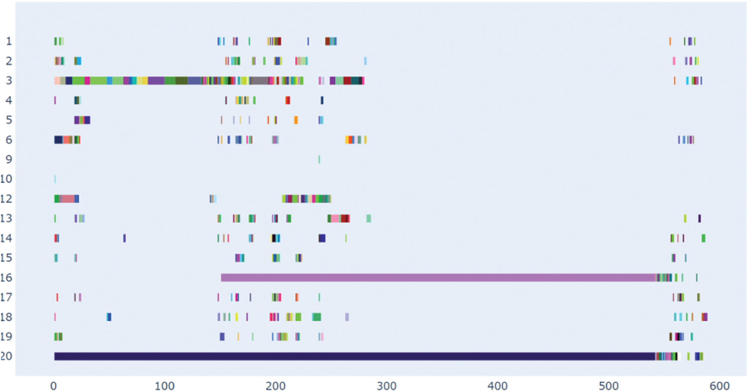
Figure 4: Generated schedule of the candidates. Vertical axis displays the workers and horizontal axis displays the time units

Tasks related to configuration and management of customer relationships and business processing support are lengthy. Fig. 5 shows the number of tasks received by each project member. Some members assigned zero or one tasks can be removed from the project candidates list, depending on conditions.

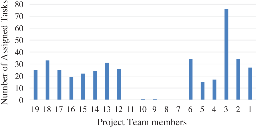
Figure 5: Number of assigned tasks to corresponding project team members

To test whether the proposed algorithm can find global solutions on smaller datasets, we created a smaller dataset with nine tasks, two candidates, and six skills from the standard dataset, then we compared the brute-force results with the proposed GA. The comparison results are shown in Tab. 2. The GA and the exhausting algorithm result return the same fitness values.

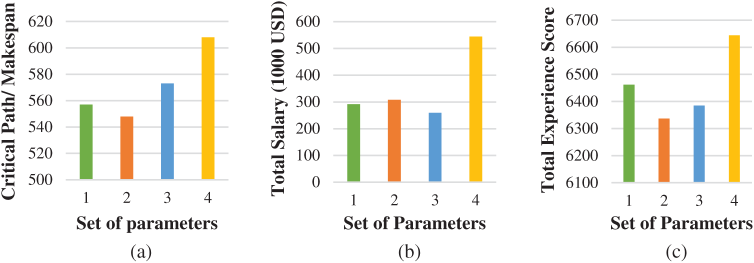
Figure 6: Execute algorithm with different parameters. (a) Shows the critical path/makespan values (O1) corresponding to different sets of parameters. (b) Displays the total salary (O2) corresponding to different sets of parameters. (c) Illustrates the sum of experience scores (O3) of hired candidates on their assigned tasks. Green Chart w1=1,w2=1,w3=1; Orange Chart w1=20,w2=1,w3=1; Blue Chart w1=1,w2=20,w3=1; Yellow Chart w1=1,w2=1,w3=20

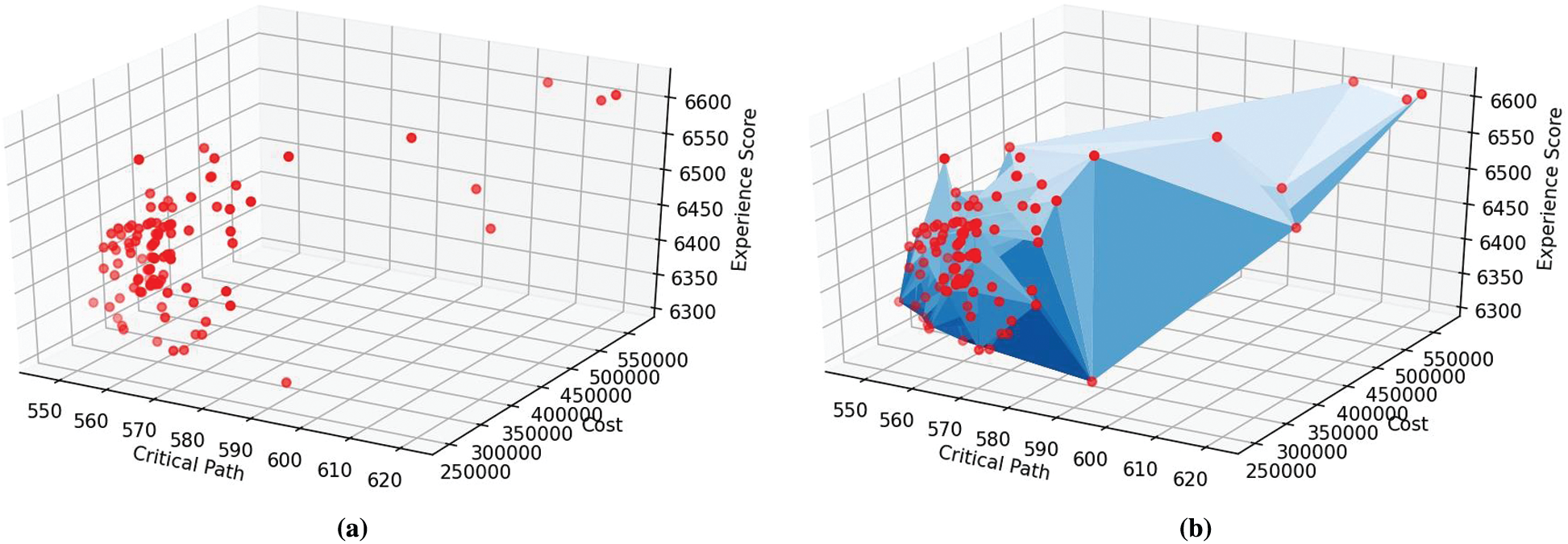
Figure 7: Collected solutions corresponding to 100 executions with different weighted parameters: (a) Solutions in the decision space; (b) Practical Pareto frontier obtained from 100 solutions in the decision space

Suppose decision-makers want to define preferences based on different objectives. They may change the values of weight parameters wi to meet different expectations. Fig. 6 illustrates the returned results using different sets of parameters for various preferences. The objective is to minimize critical path (O1), so the green bar shows the lowest value when the weight w1 is at its maximum. The minimum value of total cost (O2) is achieved with a greater value of w2 (blue bar). The third target function maximizes full experience scores (O3), so a greater value of w3 increases the score (orange bar).

To illustrate a solution space, we executed the algorithm 100 times with different weights of each objective function. It is hard to guarantee this frontier is Pareto optimal. However, many executions with different parameters provide a visualization of solutions offered by the tool in the decision space. We can consider it as the practical version of the boundary. Fig. 7 shows the Pareto frontier constructed from the practical result.

5  Conclusions

We proposed an approach to RCPSP. The model attempts to minimize critical paths and costs, and to maintain the quality of the product. The model is subject to classical RCPSP problem constraints, and some additional conditions in real software development projects. The model’s goals are generally consistent with the project’s planning. The model integrates the similarity of tasks and employees’ available working plans, and therefore can be used generically for software projects, and not only applied to the specific cases cited.

Compared to other studies [5], the proposed approach brings two main benefits: (1) The model is formulated to allow decision-makers to understand and validate the structure. We combined both approaches to the proposed MOP, each fitting a different decision-making strategy. The weighted parameter-based method enables the decision-maker to customize the weights of target functions to flexibly achieve a final solution. Compromise programming is crucial in navigating the search, even when decision-makers cannot assign preferences to objective functions. (2) To solve the combinatorial optimization problem, we designed a new GA scheme that derives the individual fitness objective functions. Experimental results show that the introduced algorithm searches well for the solution by navigating the defined distance-based method.

The problem under consideration does not require finding solutions in spaces with large dimensions. However, optimal solutions may lie in high-dimensional space in other cases. It is challenging to visualize the Pareto frontier. In these situations, compromise programming is more suitable. We hope to refine the model to consider new goals and constraints in many situations. Recent methods of evolutionary algorithms show great promise in improving the quality of search results.

Acknowledgement: We thank LetPub (https://www.letpub.com) for its linguistic assistance during the preparation of this manuscript.

Funding Statement: The authors received no specific funding for this study.

Conflicts of Interest: The authors declare that they have no conflicts of interest to report regarding the present study.

This work is licensed under a Creative Commons Attribution 4.0 International License, which permits unrestricted use, distribution, and reproduction in any medium, provided the original work is properly cited.