DOI:10.32604/cmc.2021.017835
| Computers, Materials & Continua DOI:10.32604/cmc.2021.017835 | |
| Article |
Classification of Retroviruses Based on Genomic Data Using RVGC
1Department of CS & IT, University of Sargodha, Sargodha, 40100, Pakistan
2Department of CS & IT, University of Mianwali, Mianwali, 42200, Pakistan
3School of Systems and Technology, University of Management and Technology, Lahore, 54782, Pakistan
4Department of Computer Science, HITEC University Taxila, Taxila, Pakistan
5Department of Computer Science and Engineering, Soonchunhyang University, Asan, Korea
6Faculty of Applied Computing and Technology, Noroff University College, Kristiansand, Norway
*Corresponding Author: Yunyoung Nam. Email: ynam@sch.ac.kr
Received: 13 February 2021; Accepted: 17 April 2021
Abstract: Retroviruses are a large group of infectious agents with similar virion structures and replication mechanisms. AIDS, cancer, neurologic disorders, and other clinical conditions can all be fatal due to retrovirus infections. Detection of retroviruses by genome sequence is a biological problem that benefits from computational methods. The National Center for Biotechnology Information (NCBI) promotes science and health by making biomedical and genomic data available to the public. This research aims to classify the different types of rotavirus genome sequences available at the NCBI. First, nucleotide pattern occurrences are counted in the given genome sequences at the preprocessing stage. Based on some significant results, the number of features used for classification is reduced to five. The classification shall be carried out in two phases. The first phase of classification shall select only two features. Unclassified data in the first phase is transferred to the next phase, where the final decision is taken with the remaining three features. Three data sets of animals and human retroviruses are selected; the training data set is used to minimize the classifier’s number and training; the validation data set is used to validate the models. The performance of the classifier is analyzed using the test data set. Also, we use decision tree, naive Bayes, k-nearest neighbors, and vector support machines to compare results. The results show that the proposed approach performs better than the existing methods for the retrovirus’s imbalanced genome-sequence dataset.
Keywords: Retroviruses; machine learning; bioinformatics; classification
Viruses are the inevitable parasites that affect other cellular organisms. Therefore, they are called genetic parasites. They can only replicate when they have access to the cellular system of the host organisms. They are composed of two or three main parts. The first and important part is the genes composed of Deoxyribonucleic Acid (DNA) or Ribonucleic Acid (RNA). The second part is the protein coat that is useful for the protection of genes. Some viruses also have a third portion called an envelope, consisting of lipids surrounding the whole virus particle [1]. Most of the study has been done on the viruses that are associated with some disease. Retroviruses are composed of RNA and have reverse transcriptase (RT) gene that causes the conversion of RNA to DNA. This converted DNA is integrated with the host DNA while entering a cell. The DNA structure is made of nucleotide. Nucleotides are of four types, namely cytosine (C), thymine (T), adenine (A), and guanine (G). Therefore, DNA is a sequence of A, T, G, and C in order. For the computer scientist, this sequence of nucleotides (in order) looks like a string whose characters are taken from a set of alphabets A, T, G, C. A codon is a group of three nucleotides. There is a total of 64 different combinations of nucleotides from a set of A, T, G, and C. Different organisms have other counts of codons that can be used for computational processing in research on these organisms.
There are many databases available online that provide DNA sequences for different organisms. One of the most important and the most widely used databases is the National Center for Biotechnology Information (NCBI) database. sSome genome-sequence regions consist of statistically useful data while the other regions are either less useful or contain hardly detectable information. Genome-sequences data are used in many computational methods of statistical processing to detect the relevant region inside the genome sequences [2,3].
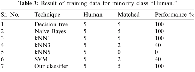
Genomic data have issues of variable dimensionality, characters with limited alphabets, and imbalanced data. The retrovirus genome sequence contains an imbalanced dataset in which the majority class has more samples than the minority class. Almost all classifiers have higher error rates on the minority class but perform well on the majority class. From a statistical point of view, this is a general problem related to almost all of the classifiers. The minority class samples may not represent their class, so their methods have a poor result on unseen data. Different techniques are used to handle the imbalanced datasets, e.g., upsampling, downsampling, etc., [4,5]. Consider two classes: diseased and healthy. The healthy class has 100 samples, and the diseased class has one sample. We can say that the majority class is −ve and the minority class is +ve in medical term. This is natural in pathology or diagnostics. Now, we have the previous knowledge that 99% of people are healthy. If we classify a sample of 1000 persons and declare all of them healthy, then the classifier’s accuracy will be 98% since the doctors found 20 of them sick. It is observed that the classifier performance is great, yet one class of experiments remained unidentified, s and therefore, the performance measure is not correct.
We can use an alternative performance measure in which we can weigh both the classes equally. It can be observed that all 980 samples of the healthy class and none of the 20 samples of the diseased class were identified correctly. So, the performance is just 50% which is bad.
This study aims to classify various types of retroviruses using DNA sequences of retrovirus available in the biomedical repository, e.g., NCBI, with the help of computational methods. The focus of this study is a similarity measure without alignment. We focus on the finding similarity measure without alignment. We observe the performance of different features and machine learning techniques for retroviral genome classification.
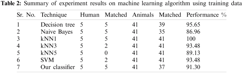
This paper has developed a two-phase algorithm to classify various types of retroviruses using DNA sequences of retrovirus available in biomedical. The performance of the classifier has been compared with some other machine learning algorithms.
The rest of the paper is organized as follows. The related work has been presented in Section 2. In Section 3, we have presented the methodology and the algorithm. Results are presented and discussed in Section 4, and the work is concluded in Section 5.
In the quest to perform retroviruses classification, a proper and well-formed database of nucleotide-sequences of retroviruses DNAs is needed. There are many resources accessible where the DNAs sequence data of retroviruses is available. A list of recent and previous databases is available at [6]. National Centre for biotechnology and information (NCBI) is one of the important resources of genetic information. Required genome sequence databases are easily available at NCBI in two forms. One of them is the Reference Sequence (RefSeq) database containing combined data for each model species of viruses. The other is GenBank containing data of each virus available publicly. The RefSeq provides a comprehensive set of useful, non-redundant, well-annotated, and explicitly connected DNAs and proteins record for each organism. Sequence records are presented in a widely accepted format and are accepted after computational validation [7]. On the other hand, GenBank provides open access and a comprehensive collection of all original sequences. Sequences discovered and approved by NCBI are grouped in a comprehensive archive [8].
Alignment based and alignment-free methods are two general types of classification methods of viruses DNA. Alignment based classification is a traditional technique based on matching DNA sequences. This method performs classification in the following three steps–-identifying conservative regions in DNA sequences in the first step. Alignment is done through insertion, deletion, and mutation in the second step. Distance measures are derived between genomes using alignment scores in the third step. Some techniques available in the literature are based on sequence alignment and derivation of alignment scores. A review of those techniques is available in [9,10]. For example, we can perform alignment between every two DNA sequences or between multiple DNA sequences simultaneously [11–16]. We can also perform alignment based on certain local DNA sequence structures [17–21] or a complete global structure of DNA sequences’ global structure. Substitution scoring matrices such as a point accepted mutation (PAM) and BLOcks Substitution Matrix (BLOSUM) and many other scoring systems have been presented to perform classification [22,23]. The proposed methods work well on small and similar DNA sequences of viruses, but there are computational and fundamental limitations on diverse and large viruses DNA sequences. In terms of computational complexity, it is infeasible to perform optimal DNA sequences’ alignment for large data set of viruses DNA sequences generated by next-generation sequencing techniques [24,25]. Alignment based method presented above requires (L2) time and space complexity, where L is the length of a sequence. More computationally efficient methods with specific properties for sequence alignment have been developed for specialized purposes, but the techniques used in these methods may not reflect the phylogeny [26,27]. The evolutionary assumption used in developing scoring methods and sequence alignment may not reflect phylogeny in fundamental virology concepts [28,29]. Simultaneously, the evolutionary method assumes linearity in scoring methods based on different scales [30]. Due to the limited number of features, these methods are combined with distance-based classifiers to develop potentially more powerful machine learning algorithms.
Alignment free methods perform viruses’ DNA sequence classification based on the degree of similarity between different features. As an alternative to alignment-based schemes or similarity score procedures, alignment-free schemes map the viral genome sequence to a feature space-point where the distance between the original sequence features helps classify the viruses [31]. Modern representation techniques perform classification using nucleotide occurrence statistics and the information about its position [32]. For example, count of k-mers, Kolmogorov complexity of sequence, absent words, matrix invariants, genomic signal processing, curves, and images [33–38]. Features selection and limited biological information are the common drawbacks of alignment-free methods. However, these methods work well in several aspects. These methods help the DNA sequence be the only available information as the associated biological knowledge required for the alignment process is not needed. Thus, no alignment is needed. These methods work well where highly diverse DNA sequences are available, and the alignment process is not trustworthy. These methods can deal with large DNA sequences datasets more efficiently as all sequences are presented in a fixed format with feature space points. Therefore, these can be used in machine learning techniques and applications such as k-nearest neighbour (k-NN) classifier, rule-based classification, support vector machine (SVM) and artificial neural network [39–42].
In the earlier study, the alignment-free methods using nucleotide statistics worked efficiently for different viruses DNA sequences but gave poor results for similar viruses DNA sequences [43]. However, in later studies, alignment-free methods work well compared to alignment-based methods with more sophisticated features, even at species levels and genus [40].
Machine learning techniques can be categorized based on distance matrices such as feature vectors and hierarchical relationship. The k-NN classifier was used to predict the label of virus DNA sequence [44,45]. The distance between the features of training data sets was calculated. The prediction was made based on the majority vote of classes in k-nearest neighbours and classes was assigned to an input DNA sequence based on the nearest distance where k-NN function was used to implement k (parameter of model) [1].
Random Forest (RF) is an assemblage technique comprising of decision tree groups. In [45], through the process of training, a large number of the uncorrelated decision trees was developed. Each tree was constructed by selecting a random subset from training virus genome-sequences data. sA random subset of characteristic variables was selected as a node based on possibility and maximum information to grow a tree. The tree was then grown by frequently splitting nodes up to the threshold. To select the label of a given DNA sequence, every tree casts a single vote for the selected class, and the one with the maximum votes was the final prediction of the RF technique
A technique was used to recognize unknown genes of related purpose from specified data by applying a support vector machine (SVM). A quality evaluation method was developed where the quality of DNA’s chromatograms was classified into low and high. The SVM classifier was used to predict two classes [45]. Machine learning techniques were presented in the quest to identify infected and actual genes, and a review of different genome data classification mechanisms by machine learning was discussed in detail [46].
A method was proposed for the global features generation of genome sequences. Human endogenous retroviruses genome-sequences were used as the data set. Infinite sequence generators were evolved to produce sequences with an augmented collection of matching blocks over a critical size in the target genome sequences. As compared to other techniques such as GC content, infinite string matching is the multiple location-based techniques. Different types of global features were selected, and genome sequences were classified using single feature threshold classifiers [47].
In [35], a DNA sequence-based species classification technique was presented. Three types of data set, i.e., iris, wine and new-thyroid, were selected for this purpose. For the development of efficient and robust classification algorithms, different DNA signature components like GC contents, exon (sum of first three nucleotides) and intron (fourth nucleotide), weight, and annealing temperatures were used as features. DNA sequence-based data classification (DSDC) was presented for species classification. It was observed that any sort of data tuning, preprocessing, and post-processing steps of data mining were not needed. It was also observed that proposed algorithms work well as compared with different differential evaluation variants. Nearest neighbors classification was used for optimization, and 1-NN was used as a performance baseline limit. The average accuracy of DSDC algorithms for the wine dataset was 74.15%, for the new thyroid dataset was 85.58%, and for iris, the dataset was 87.33%.
In [48], Fourier transform was used to generate characteristic sets based on randomness amount to classify retroviruses DNS’s sequences previously unidentified. This study used four types of data sets, including HERV, complete retroviral genome data RV, negative NRV data, and the human genome. These data sets were collected from NCBI and HERV was collected from RetroSearch. Four types of features were generated by using the Fourier phase histogram. These features were additionally applied for the analysis of RF classifier accurateness. It was observed that to distinguish retroviral genomes from non-coding sections, RF classifier produces satisfactory results.
The basic local alignment search tool (BLAST) is similar to SmithWaterman-Gotoh algorithms, but the difference is that it uses only an investigative search rather than a comprehensive search. This permits it to rum about 50 times quicker at the cost of some accurateness. It recognizes similarities (hits) amid input and query sequences and consigns scores. Overlying hits were grouped and consigned regions scores built on the BLAST scores of the sequences. Using FASTA, search regions between two stop codons were used that were long enough ( < 62 nucleotides), and these were compared to a database sof over 6000 non-retroviral and retroviral proteins. FASTA searches and BLAST searches are comparable, except that it is exclusively tuned for aligning different proteins. This database has been expanded and updated. Data is presented online in addition to data for similar regions from RepeatMasker. Often, there are perceptible alterations [49].
In preprocessing step, we count the nucleotide pattern in given DNA sequences of both human and animal retroviruses. Let
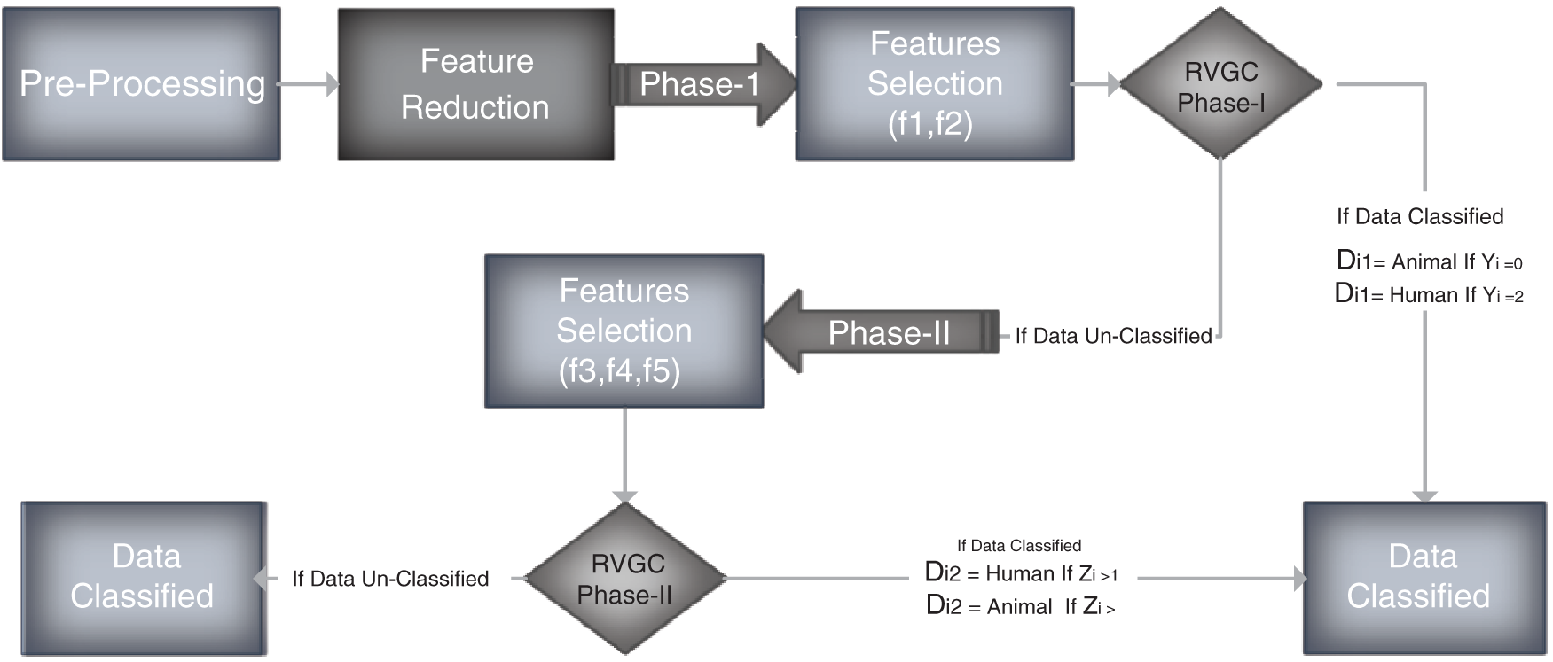
Figure 1: Flow diagram
Let hi be the ith human retroviruses samples, for
Similarly, we define
Features are in row order for
Similarly, we redefine animal data
We solved the issue of characters with limited alphabets and variable dimensionality in this step. We minimize the number of features by selecting only significant features for classification. For this purpose, the following are the details of the features reduction step. Let
Similarly,
The value 1 is assigned to
We compute
We compute
Consider the matrix
where f1, f2, f3, f4, f5 are computed as:
where f1, f2, f3, f4, f5 are column numbers of
The classification of Training data is carried out in two phases. The first part is based on features f1 and f2. The second one is based on three features, namely f3, f4 and f5.
In phase I, features f1, f2 are selected for classification. We select only selected features from the given data. We define
Similarly,
Let
Let
Now we Define
Similarly
We compute
where
All the participants with decision label Di1 “Unknown” is selected for phase II.
In phase II f3, 4, f5 are the features selected for classification.
Similarly, we define f3, f4, f5 features data for human as follow:
Let
Let
Now we define
Similarly,
We compute
We take decision
We carried out simulations with the help of
Input: Gen–-a genome
Output: D = Human/Animal
• Count # of occurrences of TCA, CTG, CAT, GTT and TAT in Gen and set them as a, b, c, d and e respectively.
• Calculate y = (138 < a < 155) + (134 < b < 169)
• If y = 2, D = Human, return
• If y = 0, D = Animal, return
• If y = 1
• Calculate z = (137 < c < 162) + (59 < d < 88) + (84 < e < 140)
• If z ¿ 1, D = Human, return
• Else D = Animal, return
Results of the classifier are presented in Tab. 1. The proposed method correctly detects 91.30% of genomes used in training data. In Phase-I of the training step, 30 from 41 animals’ retroviruses are correctly labeled as “Animal”, 2 are wrongly labeled as “Human” and 9 are labeled as “Unknown”. All human retroviruses data are classified correctly. In Phase-II of the training step, 7 from 9 animals retroviruses are correctly labeled as “Animal”, 2 are wrongly labeled as “Human”.
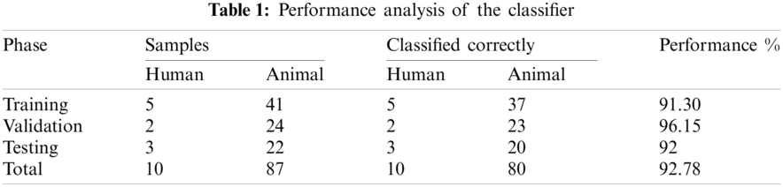
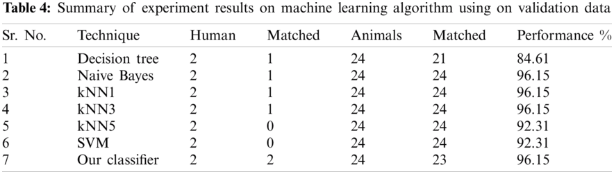
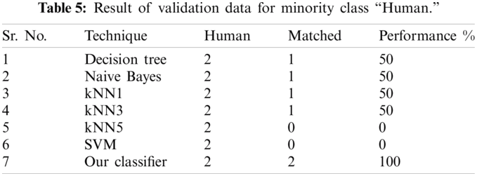
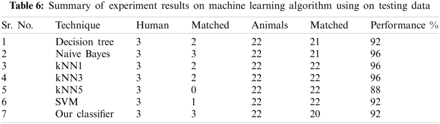
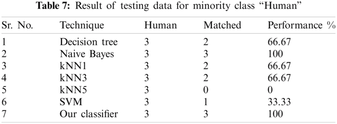
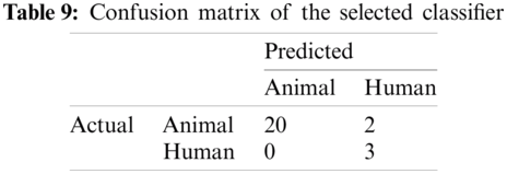
The result of the classier during the validation stage is 96.15%. In Phase-I of the validation step, 17 from 24 animal’s retroviruses are correctly labeled as “Animal”, 1 is wrongly labeled as “Human” and 6 are labeled as “Unknown”. From human data 1 is correctly labeled as “Human” and 1 is labeled as “Unknown”. In Phase-II of the validation step, 1 human and 6 animals retroviruses data are classified correctly. The result of the classifier during the testing stage is 92%. In Phase-I of the testing step, 16 from 22 animals retroviruses are correctly labeled as “Animal”, 1 is wrongly labeled as “Human” and 5 are labeled as “Unknown”. All humans are detected correctly. In Phase-II of the testing step, 4 animals retroviruses are correctly labeled as “Animal”, and 1 is wrongly labeled as “Human”. Results are given in Tabs. 1–7.
In order to check the performance of our classifier, standard performance metrics are used in this research. Given a test set with N samples, let N
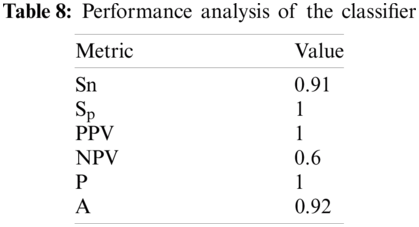
Considering Tab. 6, we have taken 22 samples from animal (N
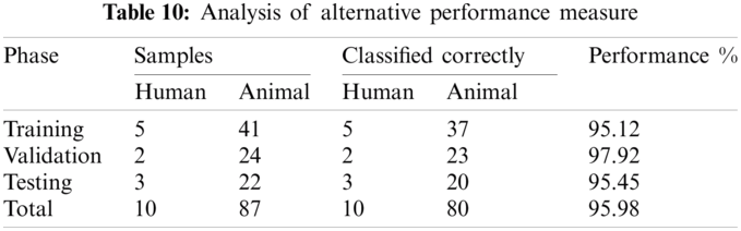
4.2 Alternate Performance Measure
We can use an alternative performance measure, as presented in the introduction chapter. Results are shown in Tab. 10. This table shows the result of an alternative performance measure.
We can use this similarity measure technique without alignments on motif-based protein-sequence, phylogenic tree construction, protein sequence analysis, clinical pathology, and other medical sciences.
• We have selected features to range based on the minimum and maximum values. Other range selection methods can also be used based on the precision of the classifier.
• We have performed a random classification technique. Another type of classification method can be used and analyzed based on the classifier’s accuracy.
• Classification can be performed in multiple phases by selecting two features in each phase up to the significant results.
• The result of the classifier can be improved by selecting mutated genes in the training stage.
In this study, we developed an algorithm for the classification of retroviruses based on DNA sequences. Firstly, the preprocessing step counts the occurrence of nucleotide patterns in given DNA sequences. Features are reduced to five based on significant results in the second step. In the final stage, classification was carried out in two-phase. In the first phase, we select two features. The given data not classified in the first phase was passed to the next phase. In the second phase, we select three features. Three data sets were selected. The first was used in training, the second was used in validation, and the third set was used to test the classifier’s performance, and the third set was used to test the classifier’s performance. The third set was used to test the classifier’s performance. It has been observed that the number of features selected provides sa significant result as compare to other combination of features. Characters with limited alphabets and variable dimensionality issues are handled using a preprocessing step. The decision of the selected threshold for the classifier in both phase provides reasonably significant results as other thresholds provide. It is observed that the selected procedure of classification gives significant result on all data sets. There is “Training”, “Validation” and “Testing”. Almost all classifiers have higher error rates on minority class but perform well on majority class. The proposed algorithm provides better results on both majority and minority classes of imbalanced data.
Funding Statement: This work was supported by the Soonchunhyang University Research Fund.
Conflicts of Interest: The authors declare that they have no conflicts of interest to report regarding the present study.
1. A. M. Q. King, M. J. Adams, E. B. Carstens and E. J. Lefkowitz, “Virus taxonomy,” in Ninth Report of the Int. Committee on Taxonomy of Viruses, California, USA, pp. 486–487, 2012. [Google Scholar]
2. Y. Cao, L. Qin, L. Zhang, J. Safrit and D. D. Ho, “Virologic and immunologic characterization of long-term survivors of human immunodeficiency virus type 1 infection,” New England Journal of Medicine, vol. 332, no. 4, pp. 201–208, 1995. [Google Scholar]
3. W. Kinsner, “Towards cognitive analysis of DNA,” in Cognitive Informatics (ICCI2010 9th IEEE Int. Conf. on Cognitive Informatics, Beijing, China, pp. 6–7, 2010. [Google Scholar]
4. M. Bekkar and T. A. Alitouche, “Imbalanced data learning approaches review,” International Journal of Data Mining and Knowledge Management Process, vol. 3, no. 4, pp. 15, 2013. [Google Scholar]
5. T. Wang, “Genome sequence-based virus taxonomy using machine learning,” Ph.D. dissertation, pp. 1–60, 2017. [Google Scholar]
6. B. Muhire, “A genome-wide pairwise-identity-based proposal for the classification of viruses in the genus mastrevirus (family geminiviridae),” Archives of Virology, vol. 158, no. 6, pp. 1411–1424, 2013. [Google Scholar]
7. J. Jurka, V. V. Kapitonov, A. Pavlicek, P. Klonowski, O. Kohany et al., “Repbase update, a database of eukaryotic repetitive elements,” Cytogenetic and Genome Research, vol. 110, no. 4, pp. 462–467, 2005. [Google Scholar]
8. T. K. Attwood, “The babel of bioinformatics,” Science, vol. 290, no. 5491, pp. 471–473, 2000. [Google Scholar]
9. L. Breiman, “Random forests,” Machine Learning, vol. 45, no. 1, pp. 5–32, 2001. [Google Scholar]
10. M. Li, J. H. Badger, X. Chen, S. Kwong, P. Kearney et al., “An information-based sequence distance and its application to whole mitochondrial genome phylogeny,” Bioinformatics, vol. 17, no. 2, pp. 149–154, 2001. [Google Scholar]
11. P.-an He and J. Wang, “Numerical characterization of DNA primary sequence,” Internet Elec. J. Mol. Des., vol. 1, pp. 668–674, 2002. [Google Scholar]
12. W. Ashlock and S. Datta, “Using Fourier phase analysis on genomic sequences to identify retroviruses,” in Proc. of the First ACM Int. Conf. on Bioinformatics and Computational Biology, New York, USA, pp. 406–409, 2010. [Google Scholar]
13. S. Henikoff and J. G. Henikoff, “Amino acid substitution matrices from protein blocks,” Proc. of the National Academy of Sciences of the United States of America, vol. 89, pp. 10915–10919, 1992. [Google Scholar]
14. M. Deng, C. Yu, Q. Liang, R. L. He and S. S.-T. Yau, “A novel method of characterizing genetic sequences: Genome space with biological distance and applications,” PloS One, vol. 6, no. 3, pp. e17293, 2011. [Google Scholar]
15. R. Durbin, S. R. Eddy, A. Krogh and G. Mitchison, “Biological sequence analysis: Probabilistic models of proteins and nucleic acids,” Cambridge, UK, pp. 1–61, 1998. [Google Scholar]
16. M. P. S. Brown, “Knowledge-based analysis of microarray gene expression data by using support vector machines,” National Academy of Sciences, vol. 97, pp. 262–267, 2000. [Google Scholar]
17. N. S. Altman, “An introduction to kernel and nearest-neighbor nonparametric regression,” The American Statistician, vol. 46, no. 3, pp. 175–185, 1992. [Google Scholar]
18. S. F. Altschul, W. Gish, W. Miller, E. W. Myers and D. J. Lipman, “Basic local alignment search tool,” Journal of Molecular Biology, vol. 215, no. 3, pp. 403–410, 1990. [Google Scholar]
19. T. Hernandez and J. Yang, “Descriptive statistics of the genome: Phylogenetic classification of viruses,” Journal of Computational Biology, vol. 23, no. 10, pp. 810–820, 2016. [Google Scholar]
20. Y.-F. Huang and C.-M. Wang, “Integration of knowledge-discovery and artificial-intelligence approaches for promoter recognition in DNA sequences,” in Third Int. Conf. on Information Technology and Applications (ICITA’05Sydney, Australia, pp. 459–464, 2005. [Google Scholar]
21. Y. Kaur and N. Sohi, “Comparison of different sequence alignment methods-a survey,” International Journal of Advanced Research in Computer Science, vol. 8, no. 5, pp. 2308–2311, 2017. [Google Scholar]
22. J. Benson, “Genbank,” Nucleic Acids Research, vol. 41, pp. D36–D42, 2013. [Google Scholar]
23. J. M. Coffin, “HIV population dynamics in vivo: Implications for genetic variation, pathogenesis, and therapy,” Science, vol. 267, pp. 483–489, 1995. [Google Scholar]
24. M. A. Larkin, “Clustal W and clustal X version 2.0,” Bioinformatics, vol. 23, pp. 2947–2948, 2007. [Google Scholar]
25. Delcher, A. Lough, J. Kasif, Fleischmann and R. Dough, “Alignment of whole genomes,” Nucleic Acids Research, vol. 27, no. 11, pp. 2369–2376, 1999. [Google Scholar]
26. P. Dixit and G. I. Prajapati, “Machine learning in bioinformatics: A novel approach for DNA sequencing,” in 2015 Fifth Int. Conf. on Advanced Computing & Communication Technologies, Haryana, India, pp. 41–47, 2015. [Google Scholar]
27. C. M. Bishop, “A critical review of machine learning of energy materials,” Advanced Energy Materials, vol. 10, vol. 22, no. 8, pp. 1903242, 2020. [Google Scholar]
28. G. Hampikian and T. Andersen, “Absent sequences: Nullomers and primes,” in Biocomputing 2007, Singapore, pp. 355–366, 2007. [Google Scholar]
29. S. B. Needleman and C. D. Wunsch, “A general method applicable to the search for similarities in the amino acid sequence of two proteins,” Journal of Molecular Biology, vol. 48, pp. 443–453, 1970. [Google Scholar]
30. W. Ashlock and S. Datta, “Fast algorithms for recognizing retroviruses,” in 2010 IEEE Int. Workshop on Genomic Signal Processing and Statistics, Cold Spring Harbor, NY, USA, pp. 1–4, 2010. [Google Scholar]
31. Baltimore and David, “Expression of animal virus genomes,” Bacteriological Reviews, vol. 35, no. 3, pp. 235, 1971. [Google Scholar]
32. B. E. Blaisdell, “A measure of the similarity of sets of sequences not requiring sequence alignment,” Proc. of the National Academy of Sciences, vol. 83, no. 14, pp. 5155–5159, 1986. [Google Scholar]
33. T. Graovac, Maja and C. Nansheng, “Using repeatmasker to identify repetitive elements in genomic sequences,” Current Protocols in Bioinformatics, vol. 25, pp. 4–10, 2004. [Google Scholar]
34. N. Cesa-Bianchi and G. Lugosi, “Fast rates for general unbounded loss functions: From ERM to generalized Bayes.” Journal of Machine Learning Research, vol. 21, no. 56, pp. 1–80, 2020. [Google Scholar]
35. O. Gotoh, “An improved algorithm for matching biological sequences,” Journal of Molecular Biology, vol. 162, no. 3, pp. 705–708, 1982. [Google Scholar]
36. M. W. Libbrecht and W. S. Noble, “Machine learning applications in genetics and genomics,” Nature Reviews Genetics, vol. 16, no. 6, pp. 321, 2015. [Google Scholar]
37. M. Lynch, “Intron evolution as a population-genetic process,” Proc. of the National Academy of Sciences, vol. 99, pp. 6118–6123, 2002. [Google Scholar]
38. E. W. Myers and W. Miller, “Optimal alignments in linear space,” Bioinformatics, vol. 4, no. 1, pp. 11–17, 1988. [Google Scholar]
39. Y. Bao, V. Chetvernin and T. Tatusova, “Improvements to pairwise sequence comparison (PASCA genome-based web tool for virus classification,” Archives of Virology, vol. 159, no. 12, pp. 3293–3304, 2014. [Google Scholar]
40. M. O. Dayhoff, R. M. Schwartz and B. C. Orcutt, “Model of evolutionary change in proteins,” Atlas of Protein Sequence and Structure, vol. 5, pp. 345–352, 1978. [Google Scholar]
41. R. C. Edgar, “MUSCLE: Multiple sequence alignment with high accuracy and high throughput,” Nucleic Acids Research, vol. 32, no. 5, pp. 1792–1797, 2004. [Google Scholar]
42. K. Katoh, K. Misawa, K. Kuma and T. Miyata, “MAFFT: A novel method for rapid multiple sequence alignment based on fast Fourier transform,” Nucleic Acids Research, vol. 30, no. 14, pp. 3059–3066, 2002. [Google Scholar]
43. B. M. Muhire, A. Varsani and D. P. Martin, “SDT: A virus classification tool based on pairwise sequence alignment and identity calculation,” PloS One, vol. 9, pp. e108277, 2014. [Google Scholar]
44. J. S. Almeida, “Sequence analysis by iterated maps, a review,” Briefings in Bioinformatics, vol. 15, pp. 369–375, 2013. [Google Scholar]
45. C. S. Leslie, E. Eskin, A. Cohen, J. Weston and W. S. Noble, “Mismatch string kernels for discriminative protein classification,” Bioinformatics, vol. 20, no. 4, pp. 467–476, 2004. [Google Scholar]
46. K. Blekas, D. I. Fotiadis and A. Likas, “Motif-based protein sequence classification using neural networks,” Journal of Computational Biology, vol. 12, pp. 64–82, 2005. [Google Scholar]
47. S. F. Altschul, “Gapped BLAST and PSI-bLAST: A new generation of protein database search programs,” Nucleic Acids Research, vol. 25, pp. 3389–3402, 1997. [Google Scholar]
48. W. Ashlock, “Detecting retroviruses in genomic sequences and applying signal processing techniques to genomics,” Literature Review, vol. 1, pp. 7–15, 2010. [Google Scholar]
49. D. Ashlock, S. Gillis and W. Ashlock, “Infinite string block matching features for DNA classification,” in 2017 IEEE Conf. on Computational Intelligence in Bioinformatics and Computational Biology, Las Vegas, Navada, pp. 1–8, 2017. [Google Scholar]
 | This work is licensed under a Creative Commons Attribution 4.0 International License, which permits unrestricted use, distribution, and reproduction in any medium, provided the original work is properly cited. |